The Volatility in a Multi-share Financial Market Model

Abstract

Single index financial market models cannot account for the empirically observed complex interactions between shares in a market. We describe a multi-share financial market model and compare characteristics of the volatility, that is the standard deviation of the price fluctuations, with empirical characteristics. In particular we find its probability distribution is similar to a log normal distribution but with a long power-law tail for the large fluctuations, and that the time development shows superdiffusion. Both these results are in good quantitative agreement with observations.

1 Introduction

Recent works have shown that financial markets cannot be completely described by single index models since they do not account for complex interactions among stocks. Share and currency cross correlation matrices show some large eigenvalues where the market and certain groups of companies/currencies move together, against a background that would be expected from Random Matrix Theorystan5 . The largest eigenvalue shows sudden increase at crashesdrozdz showing a strong global behaviour at such times. Share cross-correlations are generally positivekull . Recent resultsmant1 show more complex properties of the simultaneous distribution of individual share returns coupled in a market. These results indicate that individual stocks in a market are coupled in a complex fashion and single index models cannot account for such characteristics.

In a recent paperphysA we have described a multi-share model of a financial market and shown that it can account for some inter-share characteristics as well as for some of the now ‘well-known’ properties, such as the observation that real market returns distributions show ‘fat-tails’. That is, the returns distributions are Levy stable distributionsLP1 for the central part often characterised by a parameter $\alpha\simeq 1.4-1.7$, while the wings (after about 4 standard deviations) fall-off faster as a power-law (exponent $2\sim 5$) or possibly as a streatched exponentialstan2 ; MS1 ; stan1 ; mand1 ; M1 .

In this paper we will show by numerical simulations that this model can also account for the empirically observed properties of the volatility. Volatility is the local standard deviation of a price returns time series. The volatility distribution shows an approximate log-normal distribution for the central part but with tails that seem to follow a power law with exponent $\simeq 4$,stan3 . Furthermore volatility is known to be ‘clustered’. That is we observe bursts of relatively high volatility separated by longer periods of relatively low volatility. This intermittent behaviour is characterised by a superdiffusion with exponent $\simeq 0.7$,stan1 ; M1 .

2 Model

Here we describe the model first presented in tohwa . A more detailed discussion of its origins can be found in physA . Precursor models can be found in cha1 ; cha2 ; badhonnef .

In this model there are $N$ interacting stocks $i=1,...,N$ where for example $i=1$ refers to ‘IBM’, $i=2$ refers to ‘Disney’ etc. If we were considering the S&P500 then $N\approx 500$. Each stock is completely characterized by two variables:

1) Excess demand/supply, $s_{i}(t)$. This is a spin variable $s_{i}(t)=\pm 1$ which describes stock $i$’s current market demand/supply state. That is if $s_{i}(t)=1$ then stock $i$ is in the excess demand state at time $t$, but if $s_{i}(t)=-1$ then it is in the excess supply state. In reality excess demand/supply has magnitude as well as sign but in this extreme simplification only its sign is taken into account. This is because as explained below we are only interested in modeling the self-reinforcing persistency characteristics of each stock $i$. (This model can be easily generalized by including a excess supply/demand magnitude $g_{i}(t)$, by, say, randomly choosing the magnitude $g_{i}(t)$ from a Gaussian (or otherwise) distribution each $t$.) The price return $\Delta p_{i}(t)$ for stock $i$ at time $t$ is given by $\Delta p_{i}(t)=Ns_{i}(t)/2$. The ‘index’ price return $\Delta p(t)$ is then given by $\Delta p(t)=S(t)/2$ where $S(t)=\sum_{i=1}^{N}s_{i}(t)$. This is just the usual linear relationship $dp/dt=Dem(t)-Sup(t)$, where $Dem(t)$ and $Sup(t)$ refer to the demand and supply at time $t$ respectively. (See for example Farmer ).

2) ‘Speculator Confidence’, $V_{i}(t)$ in stock $i$ at time $t$. This is a real number which describes the overall (mean) speculator expectation of the current excess demand/supply state $s_{i}(t)$ continuing to the next time step, or reversing. In this model speculators are homogenous in their views. High confidence in a stock means speculators in general expect the current demand/supply state $s_{i}(t)$ of that stock to continue, low confidence means they expect a reversal. Our confidence $V_{i}(t)$ is cumulative and should be thought of like a ‘fitness’ in ecodynamics. It is not an intrinsic property of a stock, but is defined only by the current speculators, as a result of their expectations, and of course changes with time.

There is no spatial dimension and stocks interact only through the market macrostate defined by 1) the market excess supply/demand $G(t)=S(t)/N$ where $G(t)$ is the mean-spin $G(t)=1/N\sum_{i=1}^{N}s_{i}(t)$, and 2) the market confidence (market fitness) defined by $V(t)=1/N\sum_{i=1}^{N}V_{i}(t)$. In real markets both of these are known (imperfectly) to the speculators. (In the case of the mean-confidence $V(t)$, there may just be a general ‘mood’ traders can sense.)

For the dynamics every time step $t$ we calculate $G(t)$ and $V(t)$ and then calculate the relative confidence $u_{i}(t)$ of stock $i$ given by $u_{i}(t)=V_{i}(t)-V(t)$. In this model speculators’ expectations are on average completely self-fulfilling and with probability $Q_{i}(t)=Q(u_{i}(t))$ where $Q(x)$ is given by,

$$Q(x)=\frac{1}{1+\exp(-2\beta x)}$$ (1)

the stock state $s_{i}(t)$ is reinforcing or persistent so that $s_{i}(t+1)=s_{i}(t)$, while with probability $1-Q(u_{i}(t))$ it reverses or is anti-persistent so that $s_{i}(t+1)=-s_{i}(t)$.

Therefore it is a basic assumption of this model that there are always persistent and anti-persistent stocks and we can imagine how this might occur as follows: Every time $t$, the speculators choose a pair of stocks $\alpha$ and $\beta$ from, say, the excess demand stocks so that $s_{\alpha}(t)=1$ and $s_{\beta}(t)=1$ and compare them by comparing their confidences $V_{\alpha}(t)$ and $V_{\beta}(t)$. Suppose $V_{\alpha}(t)>V_{\beta}(t)$, therefore the speculators decide to demand $\alpha$ more and to supply $\beta$ instead. Therefore $s_{\alpha}(t+1)=1$ and $s_{\beta}(t+1)=-1$. Conversely suppose the speculators are comparing stocks $\alpha$ and $\beta$ which are in excess supply with $s_{\alpha}(t)=-1$ and $s_{\beta}(t)=-1$, where $V_{\alpha}(t)>V_{\beta}(t)$, then speculators decide to continue to supply $\alpha$ while demanding $\beta$ so that $s_{\alpha}(t+1)=-1$ and $s_{\beta}(t+1)=1$. If we imagine this process of comparing stocks happening continuously we can imagine each share generally interacting with the market confidence $V(t)$ through the relative confidence $u_{i}(t)=V_{i}(t)-V(t)$ and Eqn.1 with the above $s_{i}(t)$ update dynamics becomes a plausible description. (In fact as an alternative model, to be reported separately, we can say high valued stocks $\alpha$ are persistent $s_{\alpha}(t+1)=s_{\alpha}(t)$ but instead of low-valued stocks $\beta$ being anti-persistent we could imagine that they are completely independent of the previous state such that $s_{\beta}(t+1)=\pm 1$ at random.) (We should also point out that if the idea of anti-persistent reversing demand/supply stock states seems strange so should the idea of persistent high volatility itself!)

The relative confidence $u_{i}(t)$ measures to what extent speculators have faith in the persistence of stock $i$’s state $s_{i}(t)$ compared to their belief in the persistence of the whole market $V(t)$. The ‘inverse temperature’ parameter $\beta$ in Eq.1 measures to what extent speculator expectation is self-fullfilling, that is the extent to which homogenous ‘herding’ occurs. When $\beta=\infty$ the system is deterministic and Eq.1 reduces to a step function and the state of stocks $i$, $s_{i}(t)$, with $V_{i}(t)>V(t)$ will be persistent with probability 1, while stocks $i$ with $V_{i}(t)<V(t)$ will be anti-persistent with probability 1, i.e. complete homogenous herding. In this case the speculators behave with ‘one mind’. With $\beta=0$ all states $s_{i}(t+1)$ are chosen randomly independent of $s_{i}(t)$ and speculators are therefore completely independent in their viewpoints. (We can also say equivalently that $\beta$ measures the extent to which traders know stock $i$’s confidence $V_{i}(t)$.) It is a basic assumption of this model that a single stock cannot be considered on it’s own, independently of the rest of market, speculators are always dynamically choosing. This is reminiscent of an ecosystem where a single organism cannot be considered independently of the other coevolving organisms in the system.

Figure 1: Single realization of the market index price time series $p(t)$ for $c=0.001$, $\beta=80$ and $N=200$.

In the version of this model presented here, the dynamics of the confidences $V_{i}(t)$ themselves are treated as internally defined behaviour of the model. If a stock $i$ has persistent excess demand/supply at time $t$ then we suggest speculators decrease their confidence $V_{i}(t)$ in it by a small amount $c$, ($c>0$). If on the other hand the excess demand/supply of stock $i$ is observed to reverse we say speculator confidence is coupled to the excess demand/supply state of the market $G(t)$ such that the change in confidence, $\Delta V_{i}(t)=V_{i}(t+1)-V_{i}(t)$, is given by,

$$\Delta V_{i}(t)=\left\{\begin{array}[]{ll}-c,&if\hskip 28.45274pts_{i}(t+1)=s_{i}(t)\\ s_{i}(t)G(t),&if\hskip 28.45274pts_{i}(t+1)=-s_{i}(t)\end{array}\right.$$ (2)

Therefore since $s_{i}(t)G(t)=-\Delta s_{i}(t)G(t)/2$, speculator confidence $V_{i}(t)$ in stock $i$ decreases when stock $i$’s state $s_{i}(t)$ moves into the overall market majority state as measured by $G(t)$. This means the probability of a stocks state reversing increases when it moves into the majority and decreases when it moves into the minority. This rule has some similarity to the Minority GameMG . We believe, however, that it is more appropriate for financial market modeling to increase an agent’s fitness when the agent moves into the minority, rather than when it is in the minority. As is well known, the way to make speculative money in markets is to stay in the majority but switch state into the minority just before everybody else does. (See alsoFarmer .) Of course in the Minority Game the agents are traders not stocks, but here we assert that a similar effect occurs between individual stocks and the market itself because of the effect of the coupling of the individual stocks to the overall market. This coupling is due to the collective choosing action of the background traders.

Our stock confidences $V_{i}(t)$ and the corresponding probabilities $Q_{i}(t)$ are defined in cumulative terms, through continuous changes, like cumulative fitnesses in ecodynamics. We believe this is in keeping with the way people think, traders do not simply forget their previous evaluations of the stocks, constructing probabilities anew, but rather dynamically update their perceptions, in a simple way depending on the current behaviour of the stock.

While the parameter $\beta$ measures the amount of homogeneity of speculator opinion in the market, $c$ measures the rate by which the speculators in general lose faith in a current price trend $s_{i}(t+1)=s_{i}(t)$. That is the rate by which they lose faith in a stock’s bullishness or bearishness.

The dynamic is synchronous, all $V_{i}(t)$ and $s_{i}(t)$ are updated at the same $V(t)$ and $G(t)$ according to $Q(u_{i}(t))$. For initial conditions the spins $s_{i}(0)$ are chosen randomly and the confidences $V_{i}(0)$ randomly and uniformly on $[-1,1]$.

3 Numerical Results. The Behaviour of the Volatility

In our paperphysA we describe the behaviour of the model in detail as we vary the parameters $c$ and $\beta$. As explained in that paper we believe real financial markets are described by $c\approx 0$ ($c>0$) and $\beta\approx 80$. We show in that paper that for those parameters values the price returns distributions agree very well with the empirical observations mentioned in the Introduction. A typical index price time series for $c=0.001$, $\beta=80$ and $N=200$ is shown in Fig.1. This is just defined from the cumulative changes as $p(t)=\sum_{j=1}^{t}\Delta p(j)$. Qualitatively it looks very reminiscent of a real time series, with periods of time which look like Gaussian random walks and other times which have larger fluctuations. One ‘crash’ is visible, as is a period of ‘sustained growth’.

Here we study the behaviour of the volatility for the same parameter values and compare it with real observations mentioned in the Introduction.

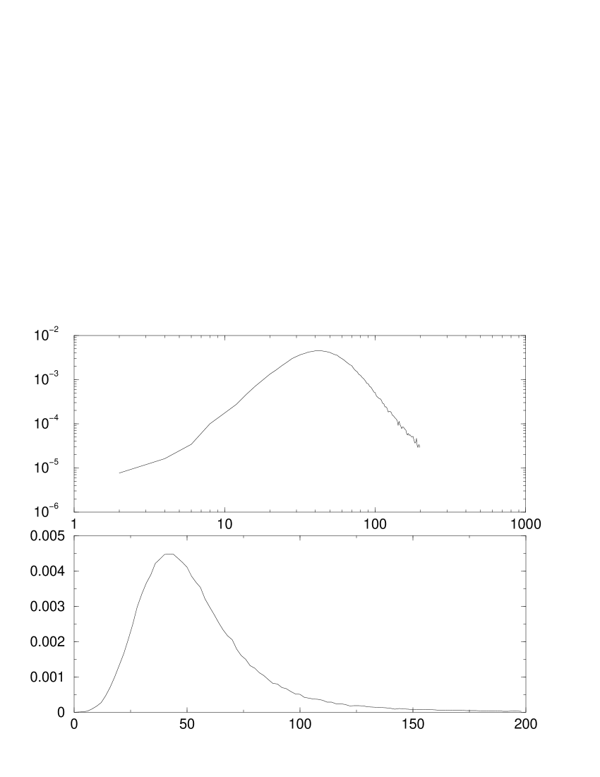
Figure 2: Distribution of absolute price changes $|\Delta p(t)_{\Delta t}|$ for $\Delta t=9$, $c=0.001$, $\beta=80$ and $N=200$. The distribution is calculated from one single realization of the price index time series. The lower panel shows the distribution in linear-linear axes, the upper panel in log-log axes.

Volatility is usually measured from financial market time series by taking a certain time window and calculating the standard deviation of the price fluctuations in that window. When considering time series of length several years the window is often of the order of a few weeks. Here, as a proxy for the volatility, we use the distribution of the absolute changes in price in a similar way tostan3 . This is shown in Fig.2 for the absolute values of $\Delta p(t)_{\Delta t=9}=\sum_{j=t}^{t+9}\Delta p(j)$. We choose to show the $\Delta t=9$ distribution, however other $\Delta t$ distributions are similar. Shown in the bottom panel is the distribution in linear-linear axes. The distribution is similar in appearance to the log-normal distribution, although it has a long tail. The distribution is shown in log-log axes in the upper panel of Fig.2. The tail is a straight line meaning the extreme absolute changes have a power-law distribution. The slope of the tail is approximately 4, in very good agreement with empirical results in stan3 , explained in the Introduction.

Next we study the dynamical behaviour of the volatilty. In physA we show that the price changes time series from this model show intermittent volatility clustering. In that paper we give some explanation for this behaviour. For our chosen parameters $c=0.001$ and $\beta=80$ the time series shows weak superdiffusion, the characteristic of persistence. Shown in Fig.3 in log-log axes is the variance $\sigma^{2}(\Delta t)$ of the price changes $\Delta p(t)_{\Delta t}$ time series, plotted against $\Delta t$. From the relationship,

$$\sigma^{2}(\Delta t)=(\Delta t)^{2\mu}$$ (3)

we obtain $2\mu\approx 1.5$ for $\Delta t\approx 1\sim 300$, while for $\Delta t>300$ we obtain $2\mu\approx 1.0$. This implies superdiffusion at shorter time scales but with reversion to normal diffusion for longer time scales. This is in very close agreement with studies in stan3 , explained in the Introduction. Also shown in Fig.3 is the same analysis for the scrambled time series, performed as a check. As expected the slope reverts to that for normal diffusion.

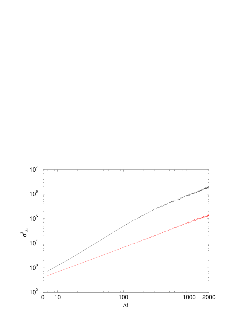
Figure 3: Diffusion of the volatility for a single realization of the price index time series with $c=0.001$, $\beta=80$ and $N=200$. The variance $\sigma^{2}(\Delta t)$ is plotted against $\Delta t$ in log-log axes. The upper curve is the results from the time series, the lower curve is from the scrambled time series.

4 Discussion

We have described a multi-share financial market model and numerically studied the behaviour of the volatility of the market index price changes $\Delta p(t)$ for the parameter values $c=0.001$ and $\beta=80$. Our results agree very well with empirical studies. In our paper physA we show these results are robust to changing the value of $c$ providing it remains ‘small’ or equivalently the system size $N$ is large. Since $c$ measures the rate at which speculators become nervous of continuing bullish or bearish trends, $c\to 0$, ($c>0$), means markets find a state where speculators try to collectively ‘stand their ground’ the longest. $\beta\approx 80$ in fact corresponds to a phase transition between a regime where price fluctuations obey Gaussian statistics and a regime where they obey Levy distributionLP1 statistics. In physA we give qualitative reasons why markets should be found in this phase transition region.

References

- (1) V.Plerou, P.Gopikrishnan, B.Rosenow, L.A.N Amaral, H.E.Stanley, Universal and Nonuniversal properties of Cross Correlations in Financial Time Series, Phys.Rev.Lett. 83 1471 (1999).
- (2) S.Drozdz, F.Grummer, F.Ruf, J.Speth, Dynamics of competition between collectivity and noise in the stock market, cond-mat/9911168
- (3) J.Kullmann, J.Kertesz, R.N.Mantegna, Identification of clusters of companies in stock indices via Potts super-paramagnetic transitions, cond-mat/0002238.
- (4) F.Lillo and R.N.Mantegna, Statistical Properties of Statistical Ensembles of Stock Returns cond-mat/9909302.
- (5) A. Ponzi and Y. Aizawa, submitted to Physica A.
- (6) M.F. Schlesinger, U. Frisch and G. Zaslavsky,(eds) Levy Flights and Related Phenomena in Physics (Springer, Berlin 1995).
- (7) V.Plerou, P.Gopikrishnan, L.A. Nunes Amaral, M.Meyer, H.E.Stanley, Scaling of the Distribution of price fluctuations of individual companies, cond-mat/9907161.
- (8) R.N Mantegna, H. Eugene Stanley, Nature 376 46-49 (1995).
- (9) P.Gopikrishnan, V.Plerou, L.A. Nunes Amaral, M.Meyer, H.E.Stanley, Scaling of the Distribution of fluctuations of financial market indices, cond-mat/9905305.
- (10) B.B Mandlebrot, J.Business 36 394-419 (1963).
- (11) R.N Mantegna, Physica A 179 232-242 (1991).
- (12) Y.Liu, P.Gopikrishnan, P.Cizeau, M.Meyer, C-K Peng, H.E.Stanley, Statistical Properties of the volatility of price fluctuations, Phys.Rev.E 60 1390 (1999).
- (13) A. Ponzi and Y. Aizawa, Chaos, Solitons and Fractals 11, (2000) 1077-1086.
- (14) A. Ponzi and Y. Aizawa, Chaos, Solitons and Fractals 11 (2000) 1739-1746.
- (15) A. Ponzi and Y. Aizawa, Proceedings of Third Tohwa Conference on Statistical Physics, cond-mat/9911428, (Nov. 1999).
- (16) A. Ponzi and Y. Aizawa, Proceedings of ‘Economic Dynamics from the Physics Point of View’, Bad Honnef, Germany, (March.2000). To appear in Physica A.
- (17) D.Challet, Y.C.Zhang, Physica A 246 407 (1997).
- (18) J.Doyne Farmer, Market Force, Ecology and Evolution.