Inhomogeneous Pairing in Highly Disordered s-wave Superconductors

Abstract

We study a simple model of a two-dimensional s-wave superconductor in the presence of a random potential in the regime of large disorder. We first use the Bogoliubov-de Gennes (BdG) approach to show that, with increasing disorder the pairing amplitude becomes spatially inhomogeneous, and the system cannot be described within conventional approaches for studying disordered superconductors which assume a uniform order parameter. In the high disorder regime, we find that the system breaks up into superconducting islands (with large pairing amplitude) separated by an insulating sea. We show that this inhomogeneity has important implications for the physical properties of this system, such as superfluid density and the density of states. We find that a finite spectral gap persists in the density of states for all values of disorder and we provide a detailed understanding of this remarkable result. We next generalize Anderson’s idea of the pairing of exact eigenstates to include an inhomogeneous pairing amplitude, and show that it is able to qualitatively capture many of the nontrivial features of the full BdG analysis. Finally, we study the transition to a gapped insulating state driven by the quantum phase fluctuations about the inhomogeneous superconducting state.

PACS numbers: 74.20.Mn 74.30.+h 74.20.-z 71.55.Jv

]

I Introduction

Studies of the interplay between localization and superconductivity in low dimensions got a boost with the possibility of growing amorphous quench condensed films of varying thicknesses and degrees of microscopic disorder and the ability to measure their transport properties in situ in a controlled manner [1, 2]. These experiments show a dramatic reduction in $T_{c}$ with increasing disorder and eventually a transition to an insulating state above a critical disorder strength beyond which resistivity increases with decreasing $T$. The data in the vicinity of the transition often seems to exhibit scaling behavior, suggesting a continuous, disorder-driven superconductor (SC) to insulator (I) quantum phase transition at $T=0$.

The physics of these highly disordered films is outside the domain of validity of the early theories of dirty superconductors, due to Anderson [3] and to Abrikosov and Gorkov [4], which are applicable only in the low disorder regime where the mean free path is much longer than the inverse Fermi wave-vector. The effect of strong disorder on superconductivity is a challenging theoretical problem, as it necessarily involves both interactions and disorder [5].

Several different theoretical approaches have been taken in the past. First, there are various mean field approaches which either extend Anderson’s pairing of time-reversed exact eigenstates or extend the diagrammatic method to high disorder regimes; see, e.g., refs. [5, 6, 7, 8, 9, 10, 11]. In much of the present work, we will also make use of mean field theories, which however differ from all previous works in a crucial aspect: we will not make any assumption about the spatial uniformity of the local pairing amplitude $\Delta$. Using the Bogoliubov-de Gennes (BdG) approach, as well as a simpler variational treatment using exact eigenstates, we will show that outside of the weak disorder regime, the spatial inhomogeneity of $\Delta$ becomes very important.

The other point of view, primarily due to Fisher and collaborators [12], has been to focus on the universal critical properties in the vicinity of the superconductor-insulator transition (SIT). These authors have argued that fermionic degrees of freedom should be unimportant at the transition, which should then be in the same universality class as dirty boson problem. As we shall see, our results on a simple fermionic model explicitly demonstrate how the electrons remain gapped through the transition, which is then indeed bosonic in nature. The SC-I transition will be shown to be driven by the quantum phase fluctuations about the inhomogeneous mean field state [13].

We begin by summarizing our main results:

(1) With increasing disorder, the distribution $P(\Delta)$ of the local pairing amplitude $\Delta({\bf r})\simeq\langle c_{\downarrow}({\bf r})c_{\uparrow}({\bf r})\rangle$ becomes very broad, eventually developing considerable weight near $\Delta\approx 0$. In contrast, conventional mean-field approaches assume a spatially uniform $\Delta$.

(2) The spectral gap in the one-particle density of states persists even at high disorder in spite of a growing number of sites with $\Delta({\bf r})\approx 0$. A detailed understanding of this surprising effect emerges from a study of the spatial variation of $\Delta({\bf r})$ which shows the formation of locally superconducting “islands” separated by a non-superconducting sea and a very special correlation between $\Delta({\bf r})$ and the BdG eigenfunctions.

(3) We generalize the ‘pairing of exact eigenstates’ to allow for an inhomogeneous pairing amplitude, and find that it provides qualitative and quantitative insight into the BdG results.

(4) There is substantial reduction in the superfluid stiffness and off-diagonal correlations with increasing disorder. However, the spatial amplitude fluctuations (in response to the random potential) by themselves cannot destroy superconductivity.

(5) We study phase fluctuations about the inhomogeneous SC state described by a quantum XY model whose parameters, compressibility and phase stiffness, are obtained from the BdG mean-field results. A simple analysis of this effective model within a self-consistent harmonic approximation leads to a transition from the superconductor to a gapped insulator.

FIG. 1.: Schematic behavior of superfluid stiffness $D_{s}$ and energy gap $E_{gap}$ as a function of temperature $T$ and disorder $V$ for the model in Eq. (2). For $V=0$, both $D_{s}$ and $E_{gap}$ vanish at the critical temperature $T_{c}$ as expected. However, for $T=0$ the behavior is very unusual with $D_{s}$ vanishing at a critical disorder $V_{c}$ but $E_{gap}$ remaining finite and even increasing with disorder at large $V$.

Schematically our main results on the disorder dependence of the spectral gap and superfluid stiffness are summarized in Fig. 1. We see that while the superfluid density $D_{s}$ decreases with increasing disorder ultimately vanishing at a critical disorder strength, the energy gap always remains finite, and shows an unusual non-monotonic behavior: it initially decreases with disorder but remains finite and even increases for large disorder. Note the difference between the finite temperature transition in the non-disordered case and the disorder driven $T=0$ transition. The $V=0$ transition at $T_{c}$ is driven at weak coupling by the collapse of the gap. In contrast the $T=0$ transition at $V_{c}$ is driven by a vanishing superfluid stifness even though the gap remains finite.

In ref. [14] we first reported in brief some of these results and compared them with earlier Quantum Monte Carlo (QMC) studies [15] of the same model. The present paper describes these calculations in detail and extends the results to much weaker coupling (the earlier work was limited to intermediate coupling with the coherence length $\xi$ of the order of the interparticle spacing). This has been made possible both by technical improvements in solving the BdG equations self consistently on larger lattices, and by the semi-analytical treatment of the pairing of exact eigenstates.

The rest of this paper is organized as follows: In section II we describe our model for the disordered SC followed by the inhomogeneous BdG mean field method in section III. This section also contains the results of the BdG solution with a detailed discussion of the disorder-dependence of various physically interesting quantities, such as pairing amplitude, density of states, energy gap, order parameter and the superfluid density. In section IV we develop the pairing of exact eigenstates theory taking into account the inhomogeneity of the pairing amplitude. Phase fluctuations are discussed in section V and the phase diagram based on our calculations is described in section VI. In section VII we make some predictions for STM measurements and discuss some open problems and conclude in section VIII.

II Model

We describe a 2D s-wave SC in the presence of non-magnetic impurities by an attractive Hubbard model with site-randomness using the Hamiltonian, ${\cal H}={\cal H_{\rm 0}}+{\cal H}_{{\rm int}}$ where

$${\cal H_{\rm 0}} = -t\sum_{<ij>,\sigma}(c_{i\sigma}^{{\dagger}}c_{j\sigma}+h.c.)+\sum_{i,\sigma}(V_{i}-\mu)n_{i\sigma}$$ (1)

$${\cal H}_{{\rm int}} = -|U|\sum_{i}n_{i\uparrow}n_{i\downarrow}$$ (2)

where $c_{i\sigma}^{{\dagger}}$ ($c_{i\sigma}$) is the creation (destruction) operator for an electron with spin $\sigma$ on a site ${\bf r}_{i}$ of a square lattice with lattice spacing $a=1$, $t$ is the near-neighbor hopping, $|U|$ is the pairing interaction, $n_{i\sigma}=c_{i\sigma}^{{\dagger}}c_{i\sigma}$, and $\mu$ is the chemical potential. The random potential $V_{i}$ models non-magnetic impurities. $V_{i}$ is an independent random variable at each site ${\bf r}_{i}$, uniformly distributed over $[-V,V]$, and $V$ thus controls the strength of the disorder.

Before proceeding, it may be worthwhile to comment on the choice of the Hamiltonian Eq. (2). The effects of Coulomb repulsion are neglected here in a spirit similar to the Anderson localization problem [16]. In spite of this simplification, Anderson localization has had a profound impact on disordered electron systems, and a complete understanding of interactions in the presence of disorder is still an open problem. Similarly the Hamiltonian we study is a minimal model containing the interplay of superconductivity and localization. For zero disorder $V=0$ it describes s-wave superconductivity and for $|U|=0$ it reduces to the (non-interacting) Anderson localization problem. We therefore feel that it is very important to first understand the physics of this simple model before putting in the additional complication of Coulomb effects; (see section VII B for further discussion).

We next comment on the choice of parameters. We have studied the model (2) for a range of parameters: $0.8\leq|U|/t\leq 8$, $0.2\leq\langle n\rangle\leq 0.875$ and a wide range of disorder on lattices of sizes up to $N=36\times 36$. In our previous letter [14] we reported results mainly for $|U|/t=4$ for two reasons: for computational ease, and to compare with earlier QMC results. Here we focus on weaker coupling for which the pure ($V=0$) system has a superfluid stiffness $D_{s}$ much greater than the spectral gap, the significance of which will become clearer below. Specifically, we will show results for $|U|/t=1.5$ and $\langle n\rangle=0.875$ on systems of typical size $24\times 24$. We have taken care to work on systems with linear dimension larger than the coherence length $\xi$ [17].

III Bogoliubov de-Gennes Mean Field Theory

We use the Bogoliubov de-Gennes (BdG) method [18] to analyze the Hamiltonian in Eq. (2). This is a mean field theory which can treat the spatial variations of the pairing amplitude induced by disorder [19], which turn out to be very important in the large disorder regime and lead to many new and unanticipated effects [14]. The mean field decomposition of the interaction term gives expectation values to the local pairing amplitude and local density

$$\Delta({\bf r}_{i})=-|U|\langle c_{i\downarrow}c_{i\uparrow}\rangle,~{}~{}~{}~{}~{}\langle n_{i\sigma}\rangle=\langle c_{i\sigma}^{{\dagger}}c_{i\sigma}\rangle$$ (3)

and yields an effective quadratic Hamiltonian

$${\cal H}_{\rm eff}=-t\sum_{<ij>,\sigma}(c_{i\sigma}^{{\dagger}}c_{j\sigma}+h.c.)+\sum_{i}(V_{i}-\tilde{\mu_{i}})n_{i\sigma}$$ (4)

$$+\sum_{i}[\Delta({\bf r}_{i})c_{i\uparrow}^{{\dagger}}c_{i\downarrow}^{{\dagger}}+\Delta^{*}({\bf r}_{i})c_{i\uparrow}c_{i\downarrow}]$$ (5)

where $\tilde{\mu_{i}}=\mu+|U|\langle n_{i}\rangle/2$ incorporates the site-dependent Hartree shift in the presence of disorder. Here $\langle n_{i}\rangle=\sum_{\sigma}\langle n_{i,\sigma}\rangle$. We discuss in detail the importance of the inhomogeneous Hartree shift in section IV. The effective Hamiltonian (5) can be diagonalized by the canonical transformations

$$c_{i\uparrow} = \sum_{n}[\gamma_{n\uparrow}u_{n}({\bf r}_{i})-\gamma_{n\downarrow}^{{\dagger}}v_{n}^{*}({\bf r}_{i})]$$ (6)

$$c_{i\downarrow} = \sum_{n}[\gamma_{n\downarrow}u_{n}({\bf r}_{i})+\gamma_{n\uparrow}^{{\dagger}}v_{n}^{*}({\bf r}_{i})]\ \cdot$$ (7)

Here $\gamma$ ($\gamma^{{\dagger}}$) is the quasiparticle destruction (creation) operator and $u_{n}({\bf r}_{i})$ and $v_{n}({\bf r}_{i})$ satisfy $\sum_{n}|u_{n}({\bf r}_{i})|^{2}+|v_{n}({\bf r}_{i})|^{2}=1$ for each ${\bf r}_{i}$. The diagonalization leads to the BdG equations

$$\left(\matrix{\hat{\xi}&\hat{\Delta}\cr\hat{\Delta}^{*}&-\hat{\xi}^{*}}\right)\left(\matrix{u_{n}({\bf r}_{i})\cr v_{n}({\bf r}_{i})}\right)=E_{n}\left(\matrix{u_{n}({\bf r}_{i})\cr v_{n}({\bf r}_{i})}\right)$$ (8)

where the excitation eigenvalues $E_{n}\geq 0$. $\hat{\xi}u_{n}({\bf r}_{i})=-t\sum_{\hat{\delta}}u_{n}({\bf r}_{i}+\hat{\delta})+(V_{i}-\tilde{\mu_{i}})u_{n}({\bf r}_{i})$ where $\hat{\delta}=\pm{\hat{\bf x}},\pm{\hat{\bf y}}$, and $\hat{\Delta}u_{n}({\bf r}_{i})=\Delta({\bf r}_{i})u_{n}({\bf r}_{i})$; and similarly for $v_{n}({\bf r}_{i})$. Expressing $c_{i\sigma}^{{\dagger}}$ ($c_{i\sigma}$) in terms of quasiparticle operators using Eq. (7) the local pairing amplitude and number density at $T=0$ defined in Eq. (3) are written in terms of the eigenvectors of the BdG matrix as

$$\Delta({\bf r}_{i}) = |U|\sum_{n}u_{n}({\bf r}_{i})v_{n}^{*}({\bf r}_{i})$$ (9)

$$\langle n_{i}\rangle = 2\sum_{n}|v_{n}({\bf r}_{i})|^{2}$$ (10)

We now solve the BdG equations, on a finite lattice of $N$ sites with periodic boundary conditions, as follows. Starting with an initial guess for the local pairing amplitude $\{\Delta({\bf r}_{i})\}$ and the local chemical potential $\{\tilde{\mu_{i}}\}$ at each site, we numerically determine (using standard LAPACK routines) the eigenvalues $E_{n}$ and eigenvectors $\left(u_{n}({\bf r}_{i}),v_{n}({\bf r}_{i})\right)$ of the BdG matrix in Eq. (8). We then compute $\{\Delta({\bf r}_{i})\}$ and $\{\langle n_{i}\rangle\}$ from Eq. (10). If these values differ from the initial choice, the whole process is iterated with a new choice of $\{\Delta({\bf r}_{i})\}$ and $\{\langle n_{i}\rangle\}$ in the BdG matrix until self-consistency is achieved and the output is identical to the input for $\langle n_{i}\rangle$ and $\Delta({\bf r}_{i})$ at each site within a certain tolerance. The chemical potential $\mu$ is determined by $1/N\sum_{i}n_{i}=\langle n\rangle$, where $\langle n\rangle$ is the given average density of electrons. Note that $\Delta({\bf r}_{i})$ and $u({\bf r}_{i}),v({\bf r}_{i})$ can be chosen to be real quantities in the absence of a magnetic field.

The number of iterations necessary to obtain self-consistency grows with disorder. We have checked that the same solution is obtained for different initial guesses. All the results are averaged over $12-15$ different realizations of the disorder for a given disorder strength.

A Local Pairing Amplitudes and Off Diagonal Long Range Order (ODLRO)

We have compared the ground state energy of the BdG solution with that obtained by forcing a uniform pairing amplitude, and found that the BdG result was always lower. In fact, the difference between the BdG and uniform energies increased with disorder, due to the greater variational freedom associated with the inhomogeneous BdG solution.

In Fig. 2 we plot the distribution $P(\Delta)$ of the self consistent local pairing amplitude $\Delta({\bf r}_{i})$ for several values of the disorder $V$. In the absence of disorder the BDG solution has a uniform pairing amplitude $\Delta_{0}\simeq 0.153t$, identical with the BCS value for $V=0$. For low disorder $V=0.1t$, the distribution $P(\Delta)$ has a sharp peak about $\Delta_{0}$, which justifies the use of a homogeneous mean field theory (MFT) (as, e.g., in the usual derivation of Anderson’s Theorem) for small disorder. With increasing disorder $V\sim 1t$, the distribution $P(\Delta)$ becomes broad and the assumption of a uniform $\Delta$ breaks down. With further increase of disorder $V\sim 2t$, $P(\Delta)$ becomes highly skewed with weight building up near $\Delta\approx 0$. Qualitatively similar behavior was also found for different choices of the attraction $U$. We found that for the same disorder strength $V$, the fluctuations in $\Delta({\bf r}_{i})$ are larger for higher values of the attraction $|U|$.

FIG. 2.: Distribution of the local pairing amplitude $\Delta({\bf r})$ from BdG calculations for various disorder strength. At low disorder the distribution $P(\Delta)$ is sharply peaked around $\Delta_{0}\approx 0.15$, the pure BCS value for $|U|=1.5t$. $P(\Delta)$ becomes broad with increasing $V$ and finally at a very large disorder gains significant weight near $\Delta\approx 0$.

The distribution of the local pairing amplitude $P(\Delta)$ should be contrasted with the distribution of local density $P(n)$, which is also inhomogeneous with increasing disorder but very distinct as shown in Fig. 3. As a function of disorder it evolves from being sharply peaked about the average $\langle n\rangle$ at low $V$ towards an almost bimodal distribution for large $V$, with sites being either empty (corresponding to high mountains in the random potential topography) or doubly occupied (in the deep valleys of the random potential). Later, we will also contrast the spatial correlations between the local pairing amplitudes and the local densities.

The off-diagonal long range order (ODLRO) is defined by the long-distance behavior of the (disorder averaged) correlation function $\langle c_{i\uparrow}^{{\dagger}}c_{i\downarrow}^{{\dagger}}c_{j\downarrow}c_{j\uparrow}\rangle\rightarrow\Delta_{\rm OP}^{2}/|U|^{2}$ for $|{\bf r}_{i}-{\bf r}_{j}|\rightarrow\infty$. In the SC state $\Delta_{\rm OP}$ is finite whereas in the non-SC state the off-diagonal correlations decay to zero at large distances so $\Delta_{\rm OP}=0$. It can be shown that $\Delta_{\rm OP}\simeq\int d\Delta\Delta P(\Delta)$, i.e., it is the average value of the local pairing amplitude. Our calculations show that $\Delta_{\rm OP}$ which is identical to $\Delta_{0}$ in the limit $V=0$, is substantially reduced by disorder as seen in Fig. 5.

FIG. 3.: The distribution of the number of electrons per site $n({\bf r})$ obtained from the BdG solution, for various disorder strengths. At low disorder the distribution is sharply peaked around the average density $\langle n\rangle=0.875$. $P(n)$ becomes broad with increasing $V$ and for large disorder evolves towards a bimodal distribution with empty and doubly-occupied sites.

B Single Particle Density of States and Energy Gap

In Fig. 4 we show the behavior of the single particle density of states (DOS) given by

$$N(\omega)=\frac{1}{N}\sum_{n,{\bf r}_{i}}[u_{n}^{2}({\bf r}_{i})\delta(\omega-E_{n})+v_{n}^{2}({\bf r}_{i})\delta(\omega+E_{n})]$$ (11)

averaged over disorder. It is seen that with increasing disorder the DOS piled up at the gap edge in the pure SC is progressively smeared out and states are pushed to higher energies. However, the gap in the spectrum remains finite.

The energy gap $E_{\rm gap}$ is obtained directly from the BdG calculation as the lowest eigenvalue of the matrix in Eq. (8). From Fig. 5, where we plot the evolution of $E_{\rm gap}$ with disorder, we see that not only does the energy gap remain finite for all disorder strengths, it even increases at high disorder! In (much of) the remainder of this section and in the following section we will present a detailed understanding of this surprising effect.

FIG. 4.: Density of States $N(\omega)$ for three disorder strengths $V$. With increasing disorder the singular pile-up at the gap edge smears out pushing states towards higher energies. Surprisingly, the spectral gap remains finite even at large $V$.

FIG. 5.: Evolution of $E_{{\rm gap}}$ and $\Delta_{{\rm OP}}$ with disorder. At $V=0$ both are same as expected; both decrease for small disorder, but, the large disorder behavior of them are quite different. Also note the non-monotonic behavior of $E_{{\rm gap}}$.

We note that this result is counterintuitive. Given the broad distribution of pairing amplitude (Fig. 2) with a large number of sites with $\Delta\approx 0$ at high disorder, one might have expected the spectral gap to also collapse. However, this expectation is based on an (incorrect) identification of the average pairing amplitude, or order parameter $\Delta_{OP}$, with the spectral gap $E_{\rm gap}$. While the two coincide at small disorder strengths, we see from Fig. 5 that the two show qualitatively different behavior at high disorder. It turns out that important insight into this puzzling phenomenon can be obtained by looking at the inhomogeneities in $\Delta({\bf r}_{i})$ in real space, as discussed below.

C Formation of Superconducting Islands

In Fig. 6 we see the evolution of the spatial distribution of the local pairing amplitude for a given realization of the random disorder potential with increasing strength of the random potential. Though the random potential $V_{i}$ is completely uncorrelated from site to site, the system generates, with increasing disorder, spatially correlated clusters of sites with large $\Delta({\bf r}_{i})$, or “SC islands”, which are separated from one another by regions with very small $\Delta({\bf r}_{i})0$. The size of the SC islands is the coherence length, controlled by the strength of the attraction $|U|$ and the disorder $V$.

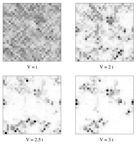
FIG. 6.: Gray-scale plot for the spatial variation of the local pairing amplitude $\Delta({\bf r})$ for a given realization of the random disorder potential, which is the same in all the panels but with increasing strength of the random potential. Note that at large $V$ the system generates “SC islands” (dark regions) with large pairing amplitude separated by an insulating “sea” (white regions) with negligible pairing amplitude.

In Fig. 7 we show density $n({\bf r}_{i})$ and $\Delta({\bf r}_{i})$ in a gray scale plot for a given realization of the random potential at a disorder strength $V=3t$. As expected the density is large in regions where the random potential is low and vice versa on a rather local scale. This is emphasized by the density-density correlations being extremely short ranged, on the scale of the lattice constant $a$. The pairing amplitude, on the other hand, shows structure i.e the formation of SC islands on the scale of the coherence length $\xi$, which is several lattice spacings. (The coherence length of the non-disordered system for this choice of $|U|$ is $\xi_{0}\simeq 10$).

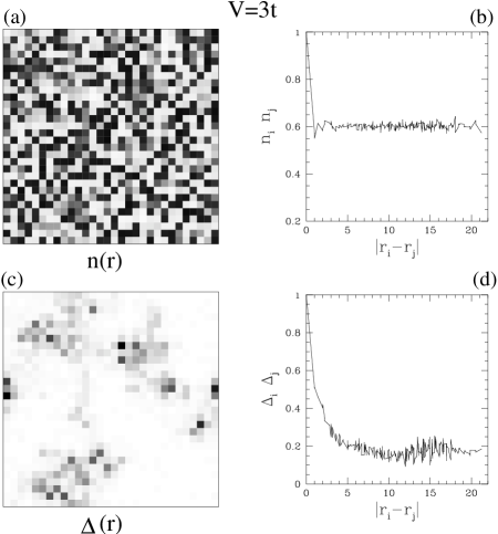
FIG. 7.: (a) Gray-scale plot of of density $n_{i}$ on the lattice at strength $V=3t$ for a given disorder realization, with darker regions indicating higher densities. (b) Plot of the density-density correlation function for the same disorder realization $n({\bf r}_{i})n({\bf r}_{j})$ as a function of the distance $r\equiv|{\bf r}_{i}-{\bf r}_{j}|$ showing that the correlations decay within a lattice constant. (c) Gray-scale plot of of pairing amplitude $\Delta({\bf r}_{i})$ on the lattice for same $V$ and same realization as in (a). (d) The correlation function $\Delta({\bf r}_{i})\Delta({\bf r}_{j})$ for this disorder realization as a function of the distance showing that the correlations persist to distances of order several lattice spacings, which is the size of the SC islands.

We next ask: where in space are these “SC islands” formed ? The will be very important in our understanding of the finite energy gap at large disorder. By correlating the locations of the islands with the underlying random potential for many different realizations, one can see that large $\Delta({\bf r})$ occurs in regions where $|V_{i}-\tilde{\mu}_{i}|$ is small. In the limit of strong disorder, this can be viewed as sort of particle-hole mixing in real space. Regions corresponding to deep valleys and to high mountains in the potential energy landscape contain fixed number of particles per site: two on a valley site or zero on a mountain site, and as a result the local pairing amplitude vanishes in such regions.

D Persistence of $E_{\rm gap}$ with Disorder

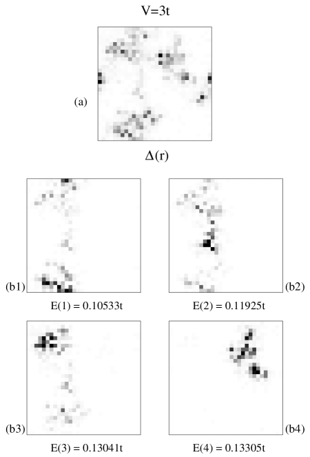
FIG. 8.: (a) Gray-scale plot of the local pairing amplitude $\Delta({\bf r}_{i})$ for a given realization of the random potential at $V=3t$. (b1-b4) Gray-scale plot of $|u_{n}({\bf r})|^{2}+|v_{n}({\bf r})|^{2}$ for the lowest four excitations ($n=1,\ldots 4$); the corresponding eigenvalues $E(1),\dots E(4)$ are also shown. Notice that a particle added to (or extracted from) the system has a high probability of being found in regions where $\Delta({\bf r}_{i})$ is large. As a consequence an energy gap persists even for high disorder.

To get a better understanding of the finite spectral gap $E_{\rm gap}$, it is useful to study the eigenfunctions corresponding to the low energy excitations. In Fig. 8 we show in gray-scale plots the local pairing amplitude $\Delta({\bf r}_{i})$ and the $|u_{n}({\bf r})|^{2}+|v_{n}({\bf r})|^{2}$ for the lowest four excited state wave functions, for a given realization of disorder at a high value of $V=3t$. We immediately notice the remarkable fact (which we have checked for many different realizations) that all the low-lying excitations live on the SC islands. Therefore it is no surprise that one ends up with a finite pairing gap.

The obvious next question is: why can one not make an even lower energy excitation which lives in the large “sea”, in between the SC islands, where one would not have to pay the cost of the pairing gap? The answer is that the random potential makes excitations in the “sea” even more energetically unfavorable than those on the SC islands. Recall from the preceding subsection that the “seas” correspond, roughly speaking, to the high mountains and deep valleys in the random potential. It is not possible to inject an electron into a deep valley as those sites are already doubly occupied, and one needs to pay a large (potential) energy cost to extract an electron from such sites. Similarly, it is energetically unfavorable to create an electron on top of a high mountain in the random potential, and it is also not possible to extract an electron from such sites as there are none.

Thus the lowest excitations must correspond to either injecting or extracting an electron from regions where $|V_{i}-\tilde{\mu}|$ is small. However, as argued above, these are precisely regions with large $\Delta({\bf r_{i}})$, and hence these excitations have a finite pairing gap. (An understanding of the non-monotonic behavior of $E_{\rm gap}$ and its eventual increase at large $V$ will come from the analysis of Section IV).

An immediate consequence of these ideas is that, while the islands may be thought of as locally superconducting, the sea separating them can be thought of as “insulating” with a large gap determined primarily by the random potential. This can be tested by the local density-of-states at different regions in the highly disordered regime as shown in Fig. 16.

E Superfluid Stiffness

It is important to understand how disorder, and in particular the formation of the inhomogeneous ground state, affects the phase rigidity. We calculate the superfluid stiffness $D_{s}$ defined by the induced current response to an external magnetic field, given by the usual Kubo formula [20]

$$\frac{D_{s}}{\pi}=\langle-k_{x}\rangle-\Lambda_{xx}(q_{x}=0,q_{y}\rightarrow 0,i\omega=0).$$ (12)

The first term $\langle-k_{x}\rangle$ is the kinetic energy along the $x$-direction and represents the diamagnetic response to an external field. (In the continuum the first term would reduce to the total density.) The second term is the paramagnetic response given by the (disorder averaged) static transverse current-current correlation function:

$$\Lambda_{xx}({\bf q},i\omega_{n})=\frac{1}{N}\int_{0}^{1/T}d\tau e^{i\omega_{n}\tau}\langle j_{x}^{p}({\bf q},\tau)j_{x}^{p}(-{\bf q},0)\rangle$$ (13)

where $j_{x}^{p}({\bf q})$ is the paramagnetic current, and $\omega_{n}=2\pi nT$.

The superfluid stiffness calculated within the BdG approximation will be denoted by $D_{s}^{0}$; (the symbol $D_{s}$ will be used for the renormalized stiffness to be defined later on). Using the BdG transformations Eq. (7) the kinetic energy can be written as $\langle-k_{x}\rangle=\frac{4t}{N}\left\langle\sum_{{\bf r},n}v_{n}({\bf r})v_{n}({\bf r}+\hat{x})\right\rangle$. A straightforward calculation of $\Lambda_{xx}$, by expressing the current operators in terms of the quasiparticle operators $\gamma$ and $\gamma^{{\dagger}}$, yields at $T=0$ the result:

$$\Lambda_{xx}(1,2,i\omega_{n}=0) = 2t^{2}\sum_{n_{1},n_{2}}\frac{1}{(E+E^{\prime})}$$ (18)

$$[v^{\prime}(2+\hat{x})u(2)+v(2+\hat{x})u^{\prime}(2)]$$

$$\times[u(1+\hat{x})v^{\prime}(1)+v(1)u^{\prime}(1+\hat{x})$$

$$-u(1)v^{\prime}(1+\hat{x})-v(1+\hat{x})u^{\prime}(1)]$$

$$+[u\leftrightarrow v,v\leftrightarrow u].$$

Here $\hat{x}$ is the unit vector along positive x-direction, and we have simplified the notation by using unprimed (primed) symbols to denote quantities with subscript $n1$ ($n2$), and $r_{i}=1,r_{j}=2$. After disorder averaging, we recover translational invariance, so that $\Lambda_{xx}({\bf r}_{i},{\bf r}_{j},0)=\Lambda_{xx}({\bf r}_{i}-{\bf r}_{j},0)$ One can then Fourier transform to ${\bf q}$ to obtain $\Lambda_{xx}(q_{x}=0,q_{y},i\omega_{n}=0)$, which can be shown to go like $A+Bq_{y}^{2}$ for small $q_{y}$. We verify this $q_{y}$-dependence in our numerical results and use it to to take the required limit in Eq. (12).

FIG. 9.: The superfluid stiffness $D_{s}^{0}/\pi$ calculated within the BdG theory as a function of disorder. The energy gap is also plotted for comparison. Note that, at $V=0$, $D_{s}^{0}\gg E_{{\rm gap}}$ a characteristic of weak-coupling superconductors. However, at large disorder one finds $D_{s}^{0}\ll E_{{\rm gap}}$ suggesting a phase fluctuation dominated regime.

In Fig. 9 we show the behavior of the BdG phase stiffness $D_{s}^{0}/\pi$ as a function of disorder. The very large reduction of $D_{s}^{0}$, by almost two orders of magnitude, can be intuitively understood by the following argument (which is also schematically illustrated in Fig. 10). Within mean field theory the phases of the order parameter at different sites are completely aligned in the ground state. When an external phase twist $\theta$ is imposed the energy of the SC increases leading to a non-zero superfluid stiffness $D_{s}^{0}\sim d^{2}E(\theta)/d\theta^{2}$. In a uniform system the external twist is uniformly distributed throughout the system. However, in an disordered system where the amplitude is highly inhomogeneous the system will distribute the phase twists non-uniformly in order to minimize energy with most of the twist accommodated in regions where the amplitude is small. Thus an inhomogeneous system will be able to greatly reduce its superfluid stiffness $D_{s}$ [21].

FIG. 10.: (a) Schematic of a disordered SC in which the non-uniform amplitude results in the formation of SC islands. Within mean field theory the phase in the ground state is spatially uniform even though the amplitude is not (larger amplitudes is represented by larger arrows). (b) Schematic illustration of the response to an externally applied phase twist (of $\pi/2$) indicated by the fat arrows. The system has a non-uniform response, with larger phase twists in regions where the amplitude is small. This results in a smaller stiffness $D_{s}^{0}\sim d^{2}E(\theta)/d\theta^{2}$ compared to the case of a uniformly distributed phase twist.

We emphasize that despite this dramatic reduction in $D_{s}^{0}$, the superfluid stiffness continues to remain non-zero within the BdG approximation. In other words, the fluctuations in the pairing amplitude alone are unable to drive the system into an insulator. In order to describe the SC-Insulator transition it is therefore essential to take into account phase fluctuations as discussed in Section V below.

F Charge Stiffness

The charge stiffness $D^{0}$ is the strength of $\delta(\omega)$ in the optical conductivity $\sigma(\omega)$ and is closely related to $D_{s}^{0}$. It is defined, after analytically continuing $\Lambda_{xx}$ to real frequency, as [20]

$$D^{0}/\pi=\langle-k_{x}\rangle-\Lambda_{xx}({\bf q}=0,\omega\rightarrow 0).$$ (19)

Note the different order of limits compared with the definition of $D_{s}$. We found $\Lambda_{xx}(0;\omega)\sim\omega^{2}$ for small $\omega$ and the resulting value of the charge stiffness is identical with the superfluid stiffness: $D^{0}=D_{s}^{0}$ for the whole range of disorder that we studied. This is to be expected in a system with a gap [20]. In fact having established this equality, we found it numerically easier to compute $D^{0}$, rather than $D_{s}^{0}$, since taking the limit $\Lambda_{xx}(\omega\rightarrow 0)$ is simpler than $\Lambda_{xx}(q_{y}\rightarrow 0)$ on a finite system.

IV Pairing of Exact Eigenstates

Although the BdG analysis described in the previous section led to various striking results, and considerable physical insight, there were a few points which could not be adequately addressed: (1) We could not study the weak-coupling limit $|U|/t\ll 1$, since the exponentially large coherence length $\xi$ leads to severe finite size effects in the numerical calculations. (2) Although the existence of the gap at large disorder could be understood, we did not get any insight into its non-monotonic dependence on disorder.

In order to address these issues, and to gain a deeper understanding of the BdG results, we now generalize Anderson’s original idea of pairing the time-reversed exact eigenstates of the disordered, noninteracting system [3], in a manner that that allows the local pairing amplitude to become spatially inhomogeneous. We will show that this generalization permits us to recover most, but not all, of the qualitative features of the BdG results. This analysis also has the virtue of leading to much simpler equations from which one can gain qualitative insights in the weak and strong disorder limit.

We begin with the noninteracting disordered problem defined by the quadratic Hamiltonian ${\cal H_{\rm 0}}$ of eq. (2). The corresponding eigenvalue problem is, in principle, soluble: ${\cal H_{\rm 0}}|\phi_{\alpha}\rangle=\varepsilon_{\alpha}|\phi_{\alpha}\rangle$, where $\alpha$ labels the exact eigenstates of ${\cal H_{\rm 0}}$. Next, following Anderson let us imagine pairing electrons in time reversed eigenstates $\alpha,\uparrow$ and ${\bar{\alpha}},\downarrow$. The analog of the “reduced BCS” Hamiltonian in this basis is then given by

$${\cal H}^{\prime}=\sum_{\alpha,\sigma}\xi_{\alpha}c_{\alpha\sigma}^{{\dagger}}c_{\alpha\sigma}-|U|\sum_{\alpha,\beta}M_{\alpha,\beta}c_{\alpha\uparrow}^{{\dagger}}c_{\bar{\alpha}\downarrow}^{{\dagger}}c_{\bar{\beta}\downarrow}c_{\beta\uparrow}$$ (20)

where the matrix $M_{\alpha,\beta}$ is defined by

$${M_{\alpha,\beta}=\sum_{{\bf r}_{i}}|\phi_{\alpha}({\bf r}_{i})|^{2}|\phi_{\beta}({\bf r}_{i})|^{2}}\ \cdot$$ (21)

Here $\xi_{\alpha}=(\varepsilon_{\alpha}-\tilde{\mu})$ is measured relative to the average Hartree shifted $\tilde{\mu}$ which fixes the electronic density. (We will return to the question of average versus site-dependent Hartree shifts later in this section.) A BCS-like mean field decomposition of the Hamiltonian (20) leads to the $T=0$ gap equation

$$\Delta_{\alpha}=|U|\sum_{\beta}M_{\alpha,\beta}\frac{\Delta_{\beta}}{2E_{\beta}}$$ (22)

where $E_{\alpha}=\sqrt{\xi_{\alpha}^{2}+\Delta_{\alpha}^{2}}$. Further, the chemical potential $\tilde{\mu}$ is determined by the number equation

$$\langle n\rangle=\frac{1}{N}\sum_{\alpha}\left(1-\frac{\xi_{\alpha}}{E_{\alpha}}\right).$$ (23)

Our formulation generalizes Anderson’s original analysis by retaining the full $M_{\alpha,\beta}$, and it is the structure of this matrix which will permit us to access the large disorder regime with highly inhomogeneous pairing.

A Non-monotonic behavior of energy gap as a function of disorder

We now solve the equations obtained above from the pairing of exact eigenstates. A qualitative analysis of the large and small disorder limits will be given and compared with a full numerical solution, and all of these results will be compared with the BdG results of the previous Section.

Let us begin with the low disorder regime. For a finite system in 2D, or an infinite system in 3D, the eigenstates $\phi_{\alpha}({\bf r}_{i})$’s are extended on the scale of system. We thus find $M_{\alpha,\beta}\approx 1/N$, independent of $\alpha$ and $\beta$, which we call the “uniform approximation” for $M$. This is this limit in which Anderson’s theorem applies, the gap equation takes the simple BCS form, and one obtains a (spatially) uniform $\Delta$.

The behavior of $E_{{\rm gap}}$ with this simplified picture is calculated and shown as “uniform approximation” in Fig. 12 for low $V$. The decrease of $E_{{\rm gap}}$ with increasing $V$ in this regime can be traced primarily to a simple density-of-states effect in the BCS result for the gap. For the nearest-neighbor dispersion in 2D and the filling chosen, one can easily show that the average DOS at the chemical potential, $\bar{N}(\xi=0)$, decreases with increasing $V$ in the weak disorder limit.

In the high disorder regime, on the other hand, the eigenstates of the non-interacting problem are strongly localized and different states have a very small spatial overlap. We can therefore make a “diagonal approximation” for for the $M$-matrix: $M_{\alpha,\beta}\approx\delta_{\alpha,\beta}\sum_{{\bf r}_{i}}|\phi_{\alpha}({\bf r}_{i})|^{4}$. We have numerically checked that the diagonal elements of $M$ are indeed the largest elements as shown in Fig. (11). Moreover, the off-diagonal elements are not important in the gap equation (22), as states which are nearby in space are far in energy and vice-versa. Next we identify $\sum_{{\bf r}_{i}}|\phi_{\alpha}({\bf r}_{i})|^{4}$ as the participation ratio for the (normalized) state $\phi_{\alpha}({\bf r}_{i})$, which in turn is given by $\zeta^{-2}_{{\rm loc}}(\alpha)$ where $\zeta_{{\rm loc}}(\alpha)$ is the localization length for that state [16].

Thus for large disorder we solve the gap equation (22) with the kernel $M_{\alpha,\beta}\approx\delta_{\alpha,\beta}\zeta^{-2}_{{\rm loc}}(\alpha)$. We find that for states $\alpha$ with energies far from the chemical potential, the solution is $\Delta_{\alpha}=0$, i.e., these states are unaffected by pairing. On the other hand, for states with small $\xi_{\alpha}$ we find $E_{\alpha}\simeq|U|/[2\zeta^{2}_{{\rm loc}}(\alpha)]$. One thus obtains a gap:

$$E_{{\rm gap}}=\frac{|U|/2}{\zeta^{2}_{{\rm loc}}}$$ (24)

in the high disorder limit, where $\zeta_{{\rm loc}}$ is the localization length at the chemical potential.

The diagonal approximation becomes exact in the extreme site localized limit ($V\rightarrow\infty$). In this case, the role of the exact eigenstate label $\alpha$ is played by the site ${\bf r}_{i}$ at which the state is localized. It is easy to show that all states for which $\xi_{r_{i}}<|U|/2$ have finite pairing amplitude and a spectral gap of $|U|/2$, which is a well known result [6].

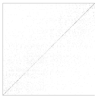
FIG. 11.: Grey-scale plot of the matrix elements of $M_{\alpha,\beta}$ at large disorder $V=6t$ for a $30\times 30$ non-interacting system. The x and y axis are the $\alpha$ and $\beta$ indices respectively. Note that diagonal matrix elements are the largest.

In Fig. 12 we compare the large disorder asymptotic result from Eq. (24), the “diagonal approximation”, with a full numerical solution of equations (22) and (23) of the method of pairing of exact eigenstates (where we self-consistently determined $\Delta_{\alpha}$’s for all $\alpha$’s and $\tilde{\mu}$). Finally we also show in Fig. 12 the BdG solution, with a uniform Hartree shift, which is in excellent agreement with the results from pairing of exact eigenstates. (Similar agreement is also found for all the other quantities like the $P(\Delta),\Delta_{{\rm OP}},N(\omega)$ and $D_{s}^{0}/\pi$ as a function of $V$)

To summarize: we now have a complete understanding of the non-monotonic dependence of the spectral gap on disorder. The weak disorder asymptotic shows that the initial drop is a simple density-of-states effect. On the other hand the increase of the gap in the strong disorder limit comes from the decrease in the localization length $\zeta_{{\rm loc}}$ as seen from Eq. (24).

It is important to emphasize that while the numerical comparisons in Fig. 12 are for a moderate value of $|U|=1.5t$, the method of pairing of exact eigenstates should work best in the weak-coupling limit, where $|U|$ is the smallest energy scale in the problem, and hence the noninteracting problem is diagonalized first. The analytical approximations in the small and large disorder limits given above are thus valid even for $|U|/t\ll 1$ where we cannot do reliable numerical calculations.

FIG. 12.: Upper Panel : Comparison of the energy gap $E_{\rm gap}$ as a function of disorder obtained by the generalized pairing of exact eigenstates method and the BdG approach. Both methods are implemented with only an average Hartree shift. Also shown are two asymptotic regimes for the gap. The decrease of $E_{\rm gap}$ at low $V$ because of the decrease of the DOS with increasing $V$ is described within a “uniform approximation” (see text) and the increase of $E_{\rm gap}$ at large disorder due to strong localization effects on the single particle wave functions is described within the “diagonal approximation” (see text). Lower Panel : Comparison of the energy gap $E_{\rm gap}$ as a function of disorder calculated within the BdG approach with an average and a site-dependent Hartree shift. While the two results are qualitatively similar, there are quantitative differences.

B Correlation between SC islands and excitations

The pairing of exact eigenstates formulation also gives analytical insight into the large spatial overlap of the low lying excited states with the SC islands in the large disorder regime, which was observed and discussed at length in the previous section.

One can show quite generally that the pairing amplitude in real space $\Delta({\bf r})$ is related to $\Delta(\alpha)$ through $\Delta_{\alpha}=\sum_{{\bf r}_{i}}\Delta({\bf r}_{i})|\phi_{\alpha}({\bf r}_{i})|^{2}$. The gap equation (22) can then be rewritten as

$$\Delta({\bf r}_{i})=\frac{|U|}{2}\sum_{\alpha}\frac{\Delta_{\alpha}}{\sqrt{\xi_{\alpha}^{2}+\Delta_{\alpha}^{2}}}|\phi_{\alpha}({\bf r}_{i})|^{2}$$ (25)

We now specialize to the large disorder regime and use the solution of the gap equation within the “diagonal approximation” in the preceding subsection to note that the only $\alpha$’s which contribute to the sum are those with $\xi_{0}\approx 0$, since otherwise $\Delta_{\alpha}=0$. The above equation then simplifies to $\Delta({\bf r}_{i})\approx|U|\sum_{\alpha}^{\prime}|\phi_{\alpha}({\bf r}_{i})|^{2}/2$ with the sum restricted to states near the chemical potential. This immediately shows the strong correlation between the spatial structures of the regions of $\Delta({\bf r}_{i})$, the SC islands, and that of the eigenstates $\phi_{\alpha}({\bf r}_{i})$ of the non-interacting problem, which are are precisely the low-lying excitations.

C Importance of site-dependent Hartree shift

Having seen the great success of the pairing of exact eigenstates in reproducing the results of the BdG analysis, we finally turn to the one important feature of the BdG analysis that is not captured in the present framework. We saw in Eq. (5) that the BdG equations incorporate site-dependent Hartree shifts, while the method of exact eigenstates did not. We now discuss what the effects of inhomogeneous Hartree terms are and why such terms are not easy to deal with in the exact eigenstates formalism. We note that we are not aware of any previous work that has looked at the effects of such inhomogeneous Hartree shifts.

First, inclusion of the site-dependent Hartree terms lead to a quantitative change in the behavior of $E_{{\rm gap}}$ as a function of $V$ as seen from the lower panel of Fig. 12. The calculation with the uniform (average) Hartree shift shows qualitatively similar non-monotonic behavior with a minimum in the gap at a slightly smaller value of $V$.

A much more dramatic effect can be seen in the density of states plotted in Fig. (13). The calculation with an average Hartree shift has a BCS-like pile-up in the DOS at the gap edge, while the result with the site-dependent shifts shows that this pile-up is completely smeared out and states are pushed out to the band tails. The occurrence of the DOS peak within the theory of pairing of exact eigenstates (with homogeneous Hartree shift) has the same origin as in BCS theory. However, all energies are measured with respect to chemical potential, and when the inhomogeneity in the Hartree shift of chemical potential is taken into account, it acts like a random perturbation which breaks the degeneracy of states near gap edge.

It would have been nice to incorporate a site-dependent Hartree shift in the theory of pairing of exact eigenstates. However, in this case the “normal state” Hamiltonian whose exact eigenstates one would have to solve for would be: ${\cal H_{\rm Normal}}=-t\sum_{<ij>,\sigma}(c_{i\sigma}^{{\dagger}}c_{j\sigma}+h.c.)+\sum_{i,\sigma}\left(V_{i}-\mu-|U|\langle n_{i}\rangle/2\right)n_{i\sigma}$. However, one then loses much of the simplicity of the exact eigenstates formalism since ${\cal H_{\rm Normal}}$ is itself an interacting problem, which needs to be solved self-consistently. Further, there are some problems (which we will not discuss here) associated with treating $U$ at the Hartree level alone, before incorporating the pairing physics, in the large disorder regime [22].

In conclusion, while the generalized pairing of exact eigenstates is able to give much insight into the behavior of the spectral gap and pairing amplitudes, and gives qualitative information about the weak coupling limit, the BdG method with site-dependent Hartree shifts is the best scheme for quantitative results.

FIG. 13.: The density of states obtained by using the pairing of exact eigenstates method using only the average Hartree shift at a disorder strength $V=2t$ in the insulator. Note the unphysical pile up of states just beyond the gap. This artifact is not present in the BdG density of states shown in Fig. (4) which includes the local Hartree shift also self consistently.

V Quantum Phase Fluctuations

As described at the end of Section III, the BdG analysis leads to a large suppression of the superfluid stiffness, but the disorder induced amplitude inhomogeneity is not sufficient to drive $D_{s}$ to zero. In order to understand the transition to an insulating state, we must focus on the phase degrees of freedom which are ignored (or frozen) in the mean field description used thus far. We thus use the 2D quantum XY action in imaginary time:

$$S_{\theta}=\frac{\kappa\xi^{2}}{8}\int_{0}^{\beta}d\tau\sum_{{\bf r}}\left(\frac{\partial\theta({\bf r},\tau)}{\partial\tau}\right)^{2}$$ (26)

$$+\frac{D_{s}^{0}}{4}\int_{0}^{\beta}d\tau\sum_{{\bf r},{\bf\delta}}(1-{\rm cos}[\theta({\bf r},\tau)-\theta({\bf r}+{\bf\delta},\tau)])$$ (27)

to describe the dynamics of the phase variables $\theta({\bf r},\tau)$ defined on a coarse-grained square lattice of lattice spacing $\xi$.

We can motivate the use of such a model in both the weak disorder limits and therefore use it for all disorder strengths. At weak disorder, one can follow the derivation of ref. [8] to derive an effective action for the phase variables in a disordered systems, and then coarse grain to the scale of $\xi$ using the method of ref. [23] to obtain the above action. This coarse graining shows that the coefficient of the time derivative term is $\xi^{2}\kappa$ in 2D where $\kappa=dn/d\mu$ is the static, long-wavelength compressibility calculated at the mean-field level, and the coefficient of the cosine term is the mean-field phase stiffness $D_{s}^{0}$.

In the opposite high disorder limit one can view (27) as simply describing a Josephson junction array of the SC islands embedded in an insulating sea as seen in Fig. 6. In this case, the first term represents the charging energy of the islands and the second term the Josephson coupling between islands. Further we are making the crude approximation of ignoring the random variations of the charging and coupling energies in this random system, and simply using the mean field values obtained from the BdG analysis. We also ignore the disorder dependence of the coherence length $\xi$, and for simplicity use its $V=0$ value $\xi_{0}$.

The nonlinearities in the cosine term lead to a renormalization of the superfluid stiffness which we calculate within the self-consistent harmonic approximation (SCHA) [24]. This is done by choosing a trial Gaussian action

$$S_{0}=\frac{\kappa\xi^{2}}{8}\int_{0}^{\beta}d\tau\sum_{{\bf r}}\left(\frac{\partial\theta({\bf r},\tau)}{\partial\tau}\right)^{2}$$ (28)

$$+\frac{D_{s}}{8}\int_{0}^{\beta}d\tau\sum_{{\bf r},{\bf\delta}}(\theta({\bf r},\tau)-\theta({\bf r}+{\bf\delta},\tau))^{2}$$ (29)

where the renormalized stiffness $D_{s}$ is determined by using the following variational principle

$$F_{\theta}\leq F_{0}+\langle S_{\theta}-S_{0}\rangle_{0}.$$ (30)

Here $F_{\theta}$ and $F_{0}$ are the free energies corresponding to the actions $S_{\theta}$ and $S_{0}$ respectively, and the expectation value $\langle\ldots\rangle_{0}$ is determined using the Gaussian $S_{0}$.

Minimizing the right hand side of eq. (30), we obtain the result

$$D_{s}=D_{s}^{0}{\rm exp}(-\langle\theta_{ij}^{2}\rangle_{0}/2).$$ (31)

Here $\langle\theta_{ij}^{2}\rangle_{0}$ is the mean square fluctuation of the near-neighbor phase difference, and is given by

$$\langle\theta_{ij}^{2}\rangle_{0}=\frac{2}{N\xi}\sum_{{\bf Q}}\left[\frac{\varepsilon_{{\bf Q}}}{D_{s}\kappa}\right]^{1/2}.$$ (32)

Here $\varepsilon_{{\bf Q}}=2[2-\cos(Q_{x})-\cos(Q_{y})]$, and the momentum sum is restricted to $Q_{i}<\pi$. Defining the renormalization factor $X=D_{s}/D_{s}^{0}$, and

$$\alpha\equiv\alpha(\kappa,D_{s}^{0},\xi)=\frac{1}{D_{s}^{0}\kappa\xi^{2}}\left(\frac{1}{N}\sum_{{\bf Q}}\varepsilon_{{\bf Q}}^{1/2}\right)^{2}$$ (33)

which depends upon all of the bare parameters of the theory, we find from eqs. (31) and (32) that $X$ is given by the solution of

$$X=\exp\left(-\sqrt{\alpha/X}\right).$$ (34)

We solve this transcendental equation to determine the renormalized $D_{s}$ a function of $V$, using as input for $\alpha$ the BdG results for the bare stiffness $D_{s}^{0}$ and compressibility $\kappa$ for each value of $V$. The BdG compressibility is plotted in Fig. 14(a). We do not have a simple physical for the small maximum in $\kappa$ at low disorder, which is a parameter dependent feature absent for larger values of $|U|$. However, our results for the renormalization of $D_{s}$ are completely insensitive to the presence or absence of this non-monotonicity.

The renormalized $D_{s}$ obtained from the SCHA is plotted in Fig. 14(b) as the full line. Quantum phase fluctuations are found to lower the stiffness and beyond a certain critical disorder drive it to zero, even though the bare (BdG) stiffness was always nonvanishing. Thus the SCHA gives a transition to a non-superconducting state, even though it is unreliable in vicinity of the transition. In particular, it predicts a first order transition at $\alpha_{{\rm crit}}=4{\rm exp}(-2)$ with a jump discontinuity of ${\rm exp}(-2)$ in the value of $X$. We believe that the order of the transition is an artifact of the approximation, although the critical disorder obtained from such a calculation is in reasonable agreement with quantum Monte Carlo results [15] for parameter values ($|U|/t=4$) for which a comparison can be made [14].

We next argue that quantum phase fluctuations do not have a significant effect on the electronic excitation spectrum. This is because the spectral gap at large disorder arises from low energy excitations that live on a SC island, which is relatively unaffected by phase fluctuations. On the other hand, as we have seen above, these fluctuations have a profound effect on suppressing the coherence between SC islands. Thus the non-superconductor in this model continues to have a finite spectral gap for one-electron excitations even after the effects of phase fluctuations are included. Thus it is an insulating state. Finally the absence of low lying electronic excitations near the transition implies that the quantum phase transition in this electronic model is in the superfluid-Bose insulator universality class [12].

FIG. 14.: (a) Left panel: The compressibility $\kappa=dn/d\mu$ as a function of disorder $V$. (b) Right Panel: Evolution of superfluid stiffness $D_{s}/\pi$ upon including the quantum phase fluctuations. The bare BdG stiffness $D_{s}^{0}$ is plotted as symbols with a dashed line through them, while the renormalized stiffness $D_{s}/\pi$ is shown by the full line. $D_{s}$ vanishes at $V_{c}=1.75t$ beyond which the system is insulating.

VI Phase Diagram

In this section we discuss the $T=0$ phase diagram for the disordered, attractive Hubbard model in the $(|U|/t,V/t)$-plane. It is known [16] that, on the $|U|=0$ axis, for all values of disorder $V\neq 0$, one has an Anderson insulator with gapless excitations in 2D. On the $V=0$ axis one simply has a crossover as a function of $|U|/t$ from a BCS superconductor to a condensate of interacting (hard core) bosons [25].

The four symbols marked in Fig. 15 are the result of BdG analysis supplemented by the simple phase fluctuation analysis described above. Despite the simplifying approximations involved, and the lack of a detailed study of finite size effects, we nevertheless believe that our results do give a reasonable qualitative idea about the critical disorder $V_{c}(U)$ separating the SC phase from an insulator with a gap in its single-particle excitation spectrum. Further our estimated $V_{c}$ at $|U|/t=4$ is in reasonable agreement  [14] with quantum Monte Carlo results [15].

FIG. 15.: Schematic phase diagram at $T=0$ of the disordered, attractive Hubbard model in the disorder $V$– attraction $|U|$ plane. The entire y-axis ($|U|/t=0$) corresponds to an Anderson insulator with gapless excitations. At finite $|U|/t$ there are two phases– a superconducting phase at low disorder and a gapped insulating phase at high disorder. Thus $U$ is a singular perturbation in that the smallest $|U|$ induces a gap. The symbols denote the critical disorder $V_{c}(U)$, separating the superconducting and the gapped insulating phases, estimated from the calculations described in the text. We argue against possibilities (b) and (c) for the form of the phase boundary in the $|U|\to 0$ limit, and suggest that $V_{c}(U\to 0)$ approaches a finite value of order unity, as shown schematically by curve (a). We find no evidence for a gapless Fermi insulator phase.

In principle, there are three possibilities for the continuation of the $V_{c}(U)$ phase boundary as $|U|/t\to 0$, a limit which we cannot address numerically. As shown in Fig. 15 these are: (a) $V_{c}(U\to 0)$ is a finite number of order unity; or (b) $V_{c}(U\to 0)$ diverges to infinity; or (c) $V_{c}(U\to 0)$ vanishes. We will now argue against (b) and (c), suggesting that (a) is in fact the correct result.

First we examine possibility (b) by looking at the case of a fixed small $|U|/t$ with $V\to\infty$. ¿From the large disorder asymptotics of the preceding Section (within the “diagonal approximation” for the matrix $M$) we found that one obtains SC islands whose size is the localization length. Thus the effective coherence length is determined by $\zeta_{{\rm loc}}$, i.e., the disorder and not by the weak coupling. Since this length scale becomes very small for large $V$, we expect phase fluctuations to destroy the long range phase coherence between the small SC islands. Thus we find it very hard for SC to persist out to very large disorder as required by the possibility (b).

Next consider possibility (c) by studying the case of a fixed, small $V$ taking the limit $|U|/t\ll 1$. Here one can just use the standard theory of dirty superconductors. The pure ($V=0$) coherence length $\xi_{0}$ is exponentially large in $|U|/t$, and even if the coherence length in the disordered problem is given by $\xi\sim\sqrt{\xi_{0}\ell}$, $\xi$ nevertheless grows as $|U|/t$ is reduced. With a growing coherence length, both amplitude and phase fluctuations are suppressed, and we cannot see how SC can be destroyed as required by the possibility (c).

There have been suggestions [26] from QMC studies of two insulating phases: a gapless “Fermi” insulator at small $|U|$ and a gapped “Bose” insulator at large $|U|$ for the model in Eq. (2). It is possible that a vanishing gap may have been observed because of the finite temperature in the simulations. We see absolutely no evidence for a “Fermi” insulator in this model, away from the $|U|=0$ line, and we have presented strong numerical evidence and arguments for a finite gap in the non-SC state for any $|U|>0$.

In the $|U|/t\gg 1$ our Hamiltonian maps on to the problem of hard core interacting bosons, with an effective hopping $t_{bose}\sim t^{2}/|U|$, in a random potential. For this problem one expects $V_{c}(|U|\to\infty)\sim t^{2}/|U|$, which gives us an understanding of the decrease in $V_{c}$ with $|U|$. Further, in this limit the insulating phase is precisely the Bose glass phase  [12].

VII Future Directions

A Prediction for STM measurement

As discussed in Sec.(III C), we find that the disordered SC consists of “SC islands” with significant pairing amplitude which are separated from the insulating sea with nearly zero pairing amplitude. Further we predict that the local energy gap in the SC islands (upper panel) should be smaller than the local gap in the insulating sea (lower panel) as seen by the nature of the local density of states (LDOS) in Fig. (16). The insulating nature of the sea is brought out by the absence of any build up of weight in the LDOS near the gap edge. It should be possible to measure the LDOS using an STM probe as has already been demonstrated in the context of magnetic impurities in s-wave superconductors [27] and with non-magnetic impurities in the high $T_{c}$ d-wave superconductors [28, 29].

B Coulomb Effects

Coulomb interactions have been typically included as an effective $\mu^{\ast}$ term in the coupling [5]. However, we expect that Coulomb interactions coupled with an inhomogeneous pairing amplitude should produce qualitatively novel effects. The effective attraction between electrons could become inhomogeneous producing regions where the pairing amplitude is suppressed with locally gapless excitations. Another possibility is that in the presence of repulsion between electrons, local moments could be formed [30] in the disordered SC which could act like magnetic impurities and be pair-breaking. This is an important direction for further study.

FIG. 16.: (a) Upper panel: The local density of states (LDOS) at sites where the pairing amplitude $\Delta$ is large. These regions correspond to the “SC-islands” which have a small local superconducting gap and a coherence peak at the gap edge. (b) Lower Panel: LDOS at sites with $\Delta\approx 0$. These regions correspond to the insulating sea showing a larger spectral gap. Also the coherence peak features at the gap edge are washed out as a result these regions show a pseudogap behavior.

VIII Conclusions

Depending on the material of the film and the type of substrate it is experimentally possible to grow two types of films– (a) nominally homogeneously disordered films [31], and (b) granular films [32, 33]. It is believed that the nature of the SC-insulator transition in these two types of films (either as a function of temperature for a given film, or as a function of film thickness at the extrapolated $T=0$ transition for a sequence of film thicknesses), is quite distinct. The transition in the so-called ‘homogeneous’ films of category (a) is believed to be driven by the collapse of the superconducting amplitude as a function of increasing temperature or disorder, whereas the transition in the granular films of category (b) is driven by the loss of phase coherence. In granular films superconductivity sets in in two steps: with decreasing temperature first the individual grains become superconducting but the Josephson coupling between grains is still weak so the film is still resistive. As the temperature is lowered the Josephson coupling is able to lock the phases of the individual grains into a globally phase coherent state at the transition temperature $T_{c}$ below which the film resistance is zero.

We have shown from our calculations that inhomogeneous ramified structures are generated even in models which are “homogeneously” disordered.

We find that a 2D homogeneously disordered SC shows a highly inhomogeneous pairing amplitude. At higher disorder, we obtain superconducting “islands” or grains which are coupled by Josephson coupling. Thus our theoretical work, as described in this paper, challenges the picture of two different paradigms to describe the SC-insulator transition – an amplitude-driven mechanism for the nominally ‘homogeneous films’ and a phase-driven mechanism for the granular films. We find instead that both amplitude and phase inhomogeneities play an important role. With increasing disorder first the amplitude inhomogeneity is important in generating weak links corresponding to small pairing amplitude. These weak links then become the active sites where Josephson coupling between the SC islands is weakened and leads to a decoupling of the phases between islands and hence a SC-I quantum phase transition.

Our calculations support the conjecture of Fisher et. al. (REFERNCE) that the SIT is in the universality class of disordered bosons, since we find that once the pairing amplitude is allowed to become inhomogeneous, there are no low lying fermionic excitations in the disordered s-wave superconductor. The transition to a gapped insulator is driven by the vanishing of the superfluid stiffness due to quantum phase fluctuations about the inhomogeneous paired state.

REFERENCES

- [1] A. Hebard, in Strongly Correlated Electronic Systems, edited by K. Bedell et al. (Addison-Wesley, 1994).
- [2] A. M. Goldman and N. Marković, Phys. Today, p39, November 1998.
- [3] P. W. Anderson, J Phys. Chem. Solids 11, 26 (1959).
- [4] A. A. Abrikosov and L. P. Gorkov, Sov. Phys. JETP 9, 220 (1959).
- [5] D. Belitz and T. Kirkpatrick, Rev. Mod. Phys. 66, 261 (1994); M. Sadovskii, Phys. Rept. 282, 225 (1997).
- [6] M. Ma and P. A. Lee, Phys. Rev. B32, 5658 (1985).
- [7] G. Kotliar and A. Kapitulnik, Phys. Rev. B33, 3146 (1986).
- [8] T. V. Ramakrishnan, Physica Scripta, T27, 24 (1989).
- [9] R. A. Smith and V. Ambegaokar, Phys. Rev. B45, 2463 (1992).
- [10] A. I. Larkin and Y. N. Ovchinnikov, Sov. Phys. JETP 34, 1144 (1972).
- [11] A. M. Finkel’stein, Physica B 197, 636 (1994).
- [12] M. P. A. Fisher, G. Grinstein and S. M. Girvin, Phys. Rev. Lett. 64, 587 (1990).
- [13] The importance of spatial amplitude fluctuations in the dirty boson problem was emphasized by: K. Sheshadri, H. R. Krishnamurthy, R. Pandit, and T. V. Ramakrishnan, Phys. Rev. Lett. 75, 4075 (1995).
- [14] A. Ghosal, M. Randeria and N. Trivedi, Phys. Rev. Lett. 81, 3940 (1998).
- [15] N. Trivedi, R. T. Scalettar and M. Randeria, Phys. Rev. B54, R3756 (1996); R. T. Scalettar, N. Trivedi, and C. Huscroft, Phys. Rev. B59, 4364 (1999).
- [16] P. A. Lee and T. V. Ramakrishnan, Rev. Mod. Phys. 57, 287 (1985).
- [17] For and , we estimate, from the asymptotic decay of the BCS pair wave-function, that the pure () limit coherence length (in units of the lattice spacing). In the presence of disorder, the coherence length can only be smaller than this estimate.
- [18] P. G. de Gennes, Superconductivity in Metals and Alloys (Benjamin, New York, 1966).
- [19] T. Xiang and J. M. Wheatley, Phys. Rev. B51, 11721 (1995); M. Franz, C. Kallin, A. J. Berlinsky, and M. I. Salkola, Phys. Rev. B56, 7882 (1997).
- [20] D. J. Scalapino, S. R. White, and S. C. Zhang, Phys. Rev. B47, 7995 (1993).
- [21] This idea can be used to obtain an upper bound on as shown in A. Paramekanti, N. Trivedi, and M. Randeria, Phys. Rev. B57, 11639 (1998).
- [22] A. Ghosal, Ph.D. Thesis, (2000), Tata Institute of Fundamental Research.
- [23] A. Paramekanti, M. Randeria, T. V. Ramakrishnan and S. S. Mandal, Phys. Rev. B62, 6786 (2000).
- [24] D. Wood and D. Stroud, Phys. Rev. B25, 1600 (1982); S. Chakravarty, G.-L. Ingold, S. Kivelson and A. Luther, Phys. Rev. Lett. 56, 2303 (1986).
- [25] For a review, see M. Randeria in Bose Einstein Condensation, edited by A. Griffin, D. Snoke and S. Stringari, (Cambridge, 1995).
- [26] C. Huscroft and R. T. Scalettar, Phys. Rev. Lett. 81, 2775 (1998).
- [27] A. Yazdani, B. A. Jones, C. P. Lutz, M. F. Crommie and D. M. Eigler, Science, 275, 1767 (1997).
- [28] T. Cren, D. Roditchev, W. Sacks, J. Klein, J. B. Moussy, C. Deville-Cavellin, and M. Lagues, Phys. Rev. Lett. 84, 147 (2000).
- [29] V. Madhavan et. al, Bull. Amer. Phys. Soc. 45, 416 (2000).
- [30] M. Milovanovic, S. Sachdev, and R. N. Bhatt, Phys. Rev. Lett. 63, 82 (1989); S. Sachdev, Phil. Trans. Roy. Soc. London, Ser. A 356, 173 (1998).
- [31] D. B. Haviland, Y.Liu, and A. M. Goldman, Phys. Rev. Lett. 62 2180 (1989); J. M. Valles, R.C. Dynes, and J.P. Garno, Phys. Rev. Lett. 69, 3567 (1992).
- [32] A. E. White, R, C. Dynes and J. P. Garno, Phys. Rev. Lett. 33 3549 (1986); H. M. Jaeger, D. B. Haviland, A. M. Goldman and B. G. Orr, Phys. Rev. Lett. 34 4920 (1986).
- [33] D. Shahar and Z. Ovadyahu, Phys. Rev. B46, 10917 (1992).