Elementary excitation families and their frequency ordering in cylindrically symmetric Bose–Einstein condensates

Abstract

We present a systematic classification of the elementary excitations of Bose–Einstein condensates in cylindrical traps in terms of their shapes. The classification generalizes the concept of families of excitations first identified by Hutchinson and Zaremba (1998) Phys. Rev. A 57 1280 by introducing a second classification number that allows all possible modes to be assigned to a family. We relate the energy ordering of the modes to their family classification, and provide a simple model which explains the relationship.

1 Introduction

Collective modes provide important signatures of the physics of Bose–Einstein condensates, and they have been intensively studied over the past few years. A large number of theoretical calculations, both numerical (e.g. [1]–[6]) and analytical (e.g. [7]–[18]), have been made based on the standard Bogoliubov treatment, and experimental observations [19]–[24] have confirmed that at very cold temperatures the Bogoliubov–de Gennes (BdG) equations provide a very accurate description of these modes. This method amounts essentially to specifying eigenmodes for a perturbative, linearized set of equations around a potential formed by the trap and the ground state condensate wave function. In this paper we use the standard BdG equations to make a systematic study of the shape of elementary modes and the relationship to their energy ordering. We note that very recent studies have incorporated finite temperature effects in order to improve accuracy at temperatures closer to the critical temperature (e.g. see [25]–[28] and references therein), however, for our purposes, the BdG equations provide an appropriate and tractable formalism.

For an isotropic trap, the spherical symmetry allows a separation into a radial wave function and spherical harmonics, thus much of the behaviour can be predicted from familiar cases in linear quantum mechanics. For axi-symmetric traps, which is the case for most experimental situations, such a separation is not possible, and a variety of techniques have been used to obtain the mode functions. In an elegant paper, Fliesser et al [16] obtained approximate analytic solutions in the hydrodynamic limit by identifying a non-trivial operator which commutes with both the eigenvalue operator of the BdG equations, and the angular momentum component along the symmetry axis. Hutchinson and Zaremba [5] obtained numerical solutions for the low-lying modes of axially symmetric traps, and studied the behaviour of these modes as the asymmetry of the trap was changed from prolate to oblate. The latter authors noticed that the lowest lying modes could be grouped into four distinct families, based on the behaviour of the mode frequency as a function of the trap asymmetry. They also showed by example how some of their modes could be identified with the modes found by Fliesser et al.

In this paper, we extend the results of Hutchinson and Zaremba, and Fliesser et al by obtaining a classification of the modes in terms of their geometrical shapes. This enables us to give a generalized definition of the mode families (which are in principle of unlimited number). Our classification into families can be expressed in terms of well defined quantum numbers, which can be directly related to the quantum numbers used by Fliesser et al. In addition, we have examined the energy ordering of the modes for the case of oblate and prolate traps, and give a simple model that relates the characteristic quasiparticle shapes to their energy ordering. This also explains the results of Hutchinson and Zaremba, that all modes in a family have the same frequency dependence on trap anisotropy.

2 Formalism

The ground state of a dilute Bose–Einstein condensate at low temperatures is well described by the Gross–Pitaevskii equation (GPE)

$$\left[\hat{H}_{0}+NU_{0}|\psi(\bi{r})|^{2}\right]\psi(\bi{r})=\mu\psi(\bi{r}),$$ (1)

where

$$\hat{H}_{0}=-\frac{\hbar^{2}}{2m}\nabla^{2}+V_{\mathrm{trap}}(\bi{r})$$ (2)

is the single-particle Hamiltonian of the trap and $N$ the number of atoms. The effective interaction strength $U_{0}$ is related to the s-wave scattering length $a$ and the atomic mass $m$ by $U_{0}=4\pi\hbar^{2}a/m$ (e.g. see [14]). The wave function $\psi(\bi{r})$ is normalized to unity according to $\int|\psi(\bi{r})|^{2}\rmd\bi{r}=1$ and the eigenvalue $\mu$ is the chemical potential of the condensate. The quasiparticle excitations on the ground state $\psi_{\mathrm{g}}(\bi{r})$ have amplitudes $u_{i}$ and $v_{i}$ determined by the Bogoliubov–de Gennes (BdG) equations

$$\eqalign{\mathcal{L}u_{i}(\bi{r})+U_{0}\psi_{\mathrm{g}}^{2}(\bi{r})v_{i}(\bi{r})&=\hbar\omega_{i}u_{i}(\bi{r})\\ \mathcal{L}v_{i}(\bi{r})+U_{0}\psi_{\mathrm{g}}^{*2}(\bi{r})u_{i}(\bi{r})&=-\hbar\omega_{i}v_{i}(\bi{r}),}$$ (3)

where $\mathcal{L}=\hat{H}_{0}+2NU_{0}|\psi_{\mathrm{g}}(\bi{r})|^{2}-\mu$ [1]. We note that the solutions $u_{i}$ and $v_{i}$ of equations (3) are not necessarily orthogonal to the ground state, although this is required in a fully quantum mechanical treatment. However, since the orthogonal excitations can readily be obtained from the solutions of equation (3) by projection [29] we will present only the direct solutions of equations (3) here.

In this paper we will consider the excitations on an anisotropic ground state of a condensate in a cylindrically symmetric harmonic trap with trapping potential

$$V_{\mathrm{trap}}(\bi{r})=\frac{1}{2}m\omega_{\mathrm{r}}^{2}[x^{2}+y^{2}+(\lambda z)^{2}],$$ (4)

where $\lambda=\omega_{\mathrm{z}}/\omega_{\mathrm{r}}$ is the anisotropy parameter of the trap. Our numerical solutions for the ground state of the GPE (1) and for the corresponding BdG equations (3) are expressed in units of the harmonic oscillator length $r_{0}=\sqrt{\hbar/2m\omega_{\mathrm{r}}}$ and energy $\hbar\omega_{\mathrm{r}}$. We will illustrate our discussions using the case of $\omega_{\mathrm{r}}=2\pi\cdot 75$ Hz and non-linearity parameter $C=NU_{0}/\hbar\omega_{\mathrm{r}}r_{0}^{3}=332$ (unless otherwise stated) though we have tested our results for a wide range of $C$ values of up to 300000. Because the wave function $v_{i}$ is in general fairly much a mirror image of $u_{i}$, and $|u_{i}|\gg|v_{i}|$ (apart from the lowest excitations) [4], we present only the wave function $u_{i}$.

3 Symmetries

For isotropic harmonic traps the ground state of the GPE has $l=0$, and so the GPE is completely separable and reduces to a one-dimensional problem in the radial coordinate $r.$ The BdG equations (for excitations on the ground state) are therefore also spherically symmetric, and thus the total angular momentum and the $z$-component of the angular momentum are conserved. This allows a separation of the angular dependence in the usual fashion by writing the quasiparticle amplitudes as $u(\bi{r})=u_{\mathrm{r}}(r)Y_{lm}(\vartheta,\varphi)$ and the equivalent for $v(\bi{r})$, where $Y_{lm}(\vartheta,\varphi)$ are spherical harmonics. Since the radial equation for the excitations does not contain any dependence on $m$, the solutions with the same $l$ and different $m$ are degenerate.

For cylindrically symmetric harmonic traps a complete separation of variables is not possible. Although the ordinary Schrödinger equation is separable in cartesian or cylindrical coordinates [30], this separation is not possible for the GPE due to the non-linear term. Nevertheless, solutions of the form

$$\psi(\bi{r})=\psi(\rho,z)\rme^{\rmi m_{\mathrm{c}}\varphi}$$ (5)

can be found, where $\rho$, $\varphi$ and $z$ denote the usual cylindrical coordinates. Then, neither the trapping potential nor $|\psi(\bi{r})|^{2}$ in the non-linear term of the GPE depend on the azimuthal angle $\varphi$ and thus $\hat{L}_{\mathrm{z}}$ and the operator $\hat{H}_{0}+NU_{0}|\psi(\bi{r})|^{2}$ of the GPE commute, so that $m_{\mathrm{c}}$ is a good quantum number. Since no further separation is possible, the equation must be solved in the two variables $\rho$ and $z$. The ground state solution of the GPE equation corresponds to $m_{\mathrm{c}}=0$.

Correspondingly the normal modes of the BdG equations will also have specific angular momentum compositions if $\psi(\bi{r})$ is given by (5). If $u_{i}(\bi{r})$ is an eigenfunction of $\hat{L}_{\mathrm{z}}$ with eigenvalue $\hbar m$, then $v_{i}(\bi{r})$ will be an eigenfunction with eigenvalue $\hbar(m-2m_{\mathrm{c}})$ [31]. Excitations on the ground state ($m_{\mathrm{c}}=0$) with $\pm|m|$ are degenerate because $m$ enters quadratically into the BdG equations in cylindrical coordinates.

The axially symmetric trap potential also has a reflection symmetry with respect to the $x$-$y$ plane, and thus the solutions to the BdG equations can be chosen to have a well-defined parity [5]. In the isotropic case, where $l$ and $m$ are good quantum numbers for the excitations, the parity is simply given by $\Pi=(-1)^{l-m}$. Hutchinson and Zaremba showed that, as the trap geometry is altered to an anisotropic one, the degenerate modes split into branches with different excitation frequencies, which emerge continously from the isotropic case (see figure 1 in reference [5]). This allowed them to associate a number $l$ with each branch depending on where it originates in the isotropic limit, even though total angular momentum is no longer a good quantum number.

4 Classification of Excitations on the Ground State

4.1 Thomas–Fermi limit

In the Thomas–Fermi limit a complete separation of variables is possible. Stringari [11] has shown that by casting the GPE into hydrodynamic form and then taking the Thomas–Fermi limit in the hydrodynamic regime (i.e. energies much smaller than the chemical potential) a second order wave equation can be derived to describe the elementary excitations. Fliesser et al [16] recognized some underlying symmetries of this equation by identifying three operators which commute with each other, and introduced three corresponding quantum numbers $(n,j,m)$ that classify the solutions completely. An explicit separation of the wave equation was achieved in cylindrical elliptical coordinates $\xi$, $\eta$ and $\varphi$, and in terms of these variables the quantum numbers represent

$n$:	order of polynomial in $\xi$ and $\eta$
$j$:	index to label different eigenvalues for fixed $n$ and $|m|\,;$
	$j$ runs from $0$ to $N=1+\mathrm{int}\left[\frac{n}{2}\right]$
$m$:	$z$-component of angular momentum.

The Thomas–Fermi approximation is known to be very accurate as a limiting case of the full solution if $Na/r_{0}\gg 1$, where $r_{0}$ is the harmonic oscillator length. In particular, the shape of the ground state wave function is very well approximated. Although the solutions of the full BdG equations do not strictly conserve these quantum numbers, we find that they exhibit in general the same patterns and symmetries, and we will show, in the appropriate regime, how the family classification scheme we develop in this paper can be related to $n,j,m$.

4.2 Families in the isotropic case

We first consider the isotropic case because then the patterns of the different mode families can be easily described in terms of Legendre polynomials. As the trap geometry is changed from spherical to cylindrical symmetry these patterns are continously modified, being squeezed in the direction of the stronger confinement, but the basic character remains recognizable.

In cylindrical coordinates the solutions for the excitations in an isotropic trap, $u(\bi{r})=u_{\mathrm{r}}(r)Y_{lm}(\vartheta,\varphi)$, can also be separated as $u(\bi{r})=u(\rho,z)\rme^{\rmi m\varphi}$. The relation

$$Y_{lm}(\vartheta,\varphi)=\frac{1}{\sqrt{2\pi}}\sqrt{\frac{2l+1}{2}\frac{(l-m)!}{(l+m)!}}P_{lm}(\cos\vartheta)\rme^{\rmi m\varphi}$$ (6)

between the spherical harmonics $Y_{lm}(\vartheta,\varphi)$ and the Legendre polynomials $P_{lm}(\cos\vartheta)$ shows that $u(\rho,z)$ is essentially the radial function $u_{\mathrm{r}}(r)$ modulated by the Legendre polynomial $P_{lm}(\cos\vartheta)$, where $\cos\vartheta=z(\rho^{2}+z^{2})^{-1/2}$ in cylindrical coordinates. In fact, it turns out that the general shape of the families is determined by the symmetries of the Legendre polynomials. We now show that the family classification suggested by Hutchinson and Zaremba can be generalized, in the isotropic case, as follows. First we assign a principal family number which is given by

$$f=l-|m|+1,$$ (7)

and then an additional number characterizing the radial function is needed to complete the classification into families. We shall introduce the nodal family number $n_{\mathrm{r}}$ for this purpose, which in the isotropic case is simply the number of nodes in the radial function. The family is given by the pair ($f,n_{\mathrm{r}}$), which together with the magnetic quantum number $m$ uniquely specifies any mode. In section 4.3 we will show how this family classification generalizes to the anisotropic case.

We illustrate the spatial character of the family assignment by considering first the excitation modes with no radial node ($n_{\mathrm{r}}=0$). We begin with the case $m\neq 0$, which we illustrate in figure 1 with contour plots of full numerical solutions of $u(\rho,z)$ for the specific case of the degenerate modes of the lowest $l=3$ excitation with $m=3,2,1$. Their principal family numbers are $f=1,2,3$ respectively. The cylindrical symmetry means that the $\rho$-$z$ dependence can be found on any plane through the $z$-axis

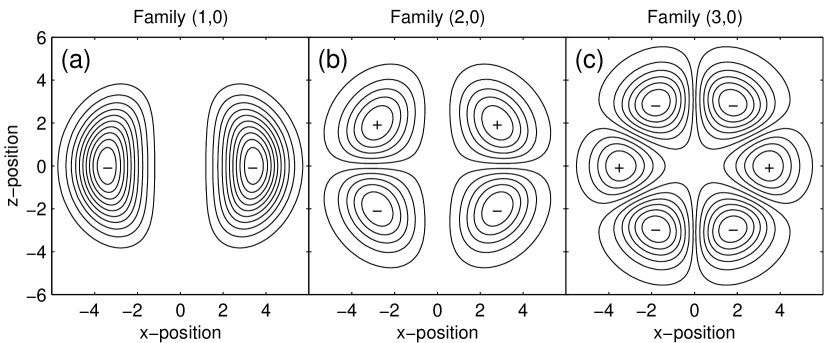
Figure 1: General shape of mode families 1 to 3 with no radial node. Contour plots in the $x$-$z$ plane of the quasiparticle amplitude $u(\rho,z)$ are given for the degenerate modes $l=3$, (a) $m=3$, (b) $m=2$, (c) $m=1$ modes.

(we have chosen the $x$-$z$ plane), and the modes are symmetric with respect to the $x$-coordinate. Since the radial function is the same for each of these modes, the relative overall shape is determined by the Legendre polynomials. The important property of the Legendre polynomials $P_{lm}(\cos\vartheta)$ for our purposes is that they have $n_{\vartheta}=l-|m|$ nodes between $0<\vartheta<\pi$. Thus, the number of angular nodal surfaces $n_{\vartheta}$ beween $0<\vartheta<\pi$, i.e. surfaces of zero density that are characterized by a constant value of $\vartheta$ in the isotropic case, determines the principal family number $f$ since $f$ is given by equation (7) as $f=l-|m|+1=n_{\vartheta}+1$. We note also that for $m\neq 0$ all Legendre polynomials are zero along the $z$-axis, but this is not a nodal surface. Because the sign of the wave function changes as it crosses a nodal surface, family 1 members have even parity, family 2 have odd parity, and in general the parity of the mode is related to the principal family number by $\Pi=(-1)^{f-1}$.

The $m=0$ member of each family has a shape that derives from the $P_{l0}$ Legendre polynomial. We call it the anomalous member of the family, since its shape differs from other members of the family only in that it is non-zero along the symmetry axis, which does not change the character of the excitation significantly. We illustrate the shape of the anomalous modes of the families $(2,0)$ and $(3,0)$ in figure 2.

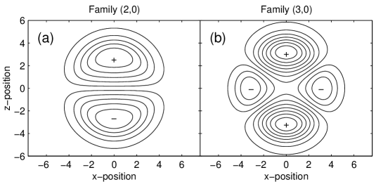
Figure 2: Contour plots in the $x$-$z$ plane of the amplitude $u(\rho,z)$ of the anomalous first members of family 2 and 3 ($m=0$).

We note also that the anomalous member of family $(1,0)$ is the ground state, which is a solution of the BdG equations [29].

The case where the radial function has a non-zero number of nodes (i.e. $n_{\mathrm{r}}\neq 0$) can now be easily visualized. The principal family number $f$ determines the number of angular nodal surfaces $(f-1)$ between $0<\vartheta<\pi$, while $n_{\mathrm{r}}$ determines the number of radial nodal surfaces, which intersect the angular nodal surfaces. In the isotropic case they are spherical and centered on the origin. In figure 3 we illustrate the first two modes having one node in the radial function,

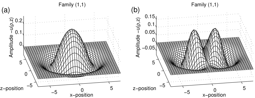
Figure 3: Family 1 with one radial node ($n_{\mathrm{r}}=1$). (a) Anomalous first member ($l=0$, $m=0$), (b) general shape (here $l=1$, $m=1$).

which both belong to the family $(1,1)$. The mode in figure 3 (a) is the anomalous first member of this family ($m=0$), while all other modes of this family have the general shape shown in figure 3 (b), which can be recognized as the same shape as in figure 1 (a), but with one radial node.

We stress that all members of the same family, apart from the anomalous one, have the same general shape, i.e. the same number of peaks (in the contour plot) in similar spatial distribution. The main qualitative difference between modes of the same family is that the peaks move radially outwards and become narrower in both radial and azimuthal direction with increasing eigenfrequency. We also note that in the isotropic case the principal family number $f$ can be readily obtained from the contour plots by counting the peaks in the half-plane $x\geq 0$ if there is no radial node ($n_{\mathrm{r}}=0$), or counting the peaks in the region that is enclosed by the $z$-axis and the $n_{\mathrm{r}}=1$ radial nodal surface if $n_{\mathrm{r}}>0$. For $m=0$ all peaks centred on the $z$-axis must also be included.

To illustrate the mode classification by family and $m$ value, we list in table 1 the 18 lowest lying modes for the $C=332$ case in an isotropic harmonic trap.

Table 1: Lowest quasiparticle modes of a condensate in an isotropic trap for $C=332$, listed by family.

• Mode				Family
  $l$	$m$	$\omega$		$f$	$n_{\mathrm{r}}$
  ​0	0	0.000		1	0
  1	0	1.000		2	0
  	1			1	0
  2	0	1.545		3	0
  	1			2	0
  	2			1	0
  3	0	2.115		4	0
  	1			3	0
  	2			2	0
  	3			1	0

  Mode				Family
  $l$	$m$	$\omega$		$f$	$n_{\mathrm{r}}$
  ​0	0	2.187		1	1
  4	0	2.748		5	0
  	1			4	0
  	2			3	0
  	3			2	0
  	4			1	0
  1	0	2.879		2	1
  	1			1	1

4.3 Anisotropic case

The main value of the concept of families is in its extension to the anisotropic cylindrically symmetric case. Hutchinson and Zaremba identified the first four families by the dependence of the eigenvalue on trap anisotropy. Here, we show that the mode topology determines the family.

In figure 4 we have plotted the quasiparticle wave functions for three families: the anomalous member of the ($3,0$) family, and the ($2,1$) and ($3,1$) families, for the case of prolate, spherical and oblate traps.

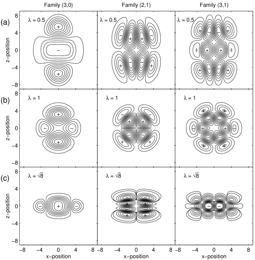
Figure 4: Effects of trap anisotropy on quasiparticle shapes. Left hand column $f=3$, $n_{\mathrm{r}}=0$, $m=0$ mode; middle column $f=2$, $n_{\mathrm{r}}=1$, $m=1$ mode; right hand column $f=3$, $n_{\mathrm{r}}=1$, $m=1$ mode. The anisotropy parameter is (a) $\lambda=0.5$, (b) $\lambda=1$, (c) $\lambda=\sqrt{8}$.

These graphs illustrate the general features that are found in the anisotropic case of cylindrical symmetry. We see that just as for the ground state of the GPE the quasiparticles are squeezed in the direction of the stronger confinement of the trap and expand in the other direction. For $\lambda<1$ (prolate) they are compressed in the $\rho$-direction and for $\lambda>1$ (oblate) they are squeezed in the $z$-direction. This distortion has no effect on the zero line along the symmetry axis, but the nodal surfaces of the isotropic case are distorted. The radial nodal surfaces are no longer spherical, but are changed to a shape that approximately follows the equipotentials of the trap. In all cases the total number of nodal crossings along the positive half of the axis of strong confinement remains exactly $n_{\mathrm{r}}$. The angular nodal surfaces can no longer be parameterized by constant $\vartheta$, and they do not meet at the origin: in the prolate case they generally intersect the symmetry axis at various (non-zero) values of $z$, while in the oblate case they generally intersect the $z=0$ plane in circles of different radii. We will call the former planar nodal surfaces and the latter cylindrical nodal surfaces, which is a good description in highly anisotropic traps as we will see in section 5.1. Exceptions are rare and occur for the case where the trap is close to spherical. Then, it is possible in the prolate case that adjacent planar nodal surfaces join just before meeting the $z$-axis, while in the oblate case it is possible that adjacent cylindrical nodal surfaces join just before the $z=0$ plane.

The nodal crossings of the isotropic case, which are at the centre of four peaks of alternating sign, can also change character in the anisotropic case, as illustrated in the right hand column of figure 4 (a). There we see that pairs of peaks of the same sign can begin fusing; in other words the crossing has become a saddle point, or ‘anti-crossing’. Despite these distortions, the character of the isotropic excitations remains clearly evident in the anisotropic case, and thus a family assignment can be made. The first step is to determine the number of radial nodes (by inspection along the positive part of the axis of strong confinement), which gives the radial family number $n_{\mathrm{r}}$. Next, if there is no radial node (i.e. $n_{\mathrm{r}}=0$), we count the number $n_{\mathrm{p}}$ of distinct peaks in a single quadrant (including peaks that are centered on the axes). If a radial node does exist, we identify the first radial nodal surface, and count the number $n_{\mathrm{p}}$ of distinct peaks in a single quadrant inside this radial nodal surface. In either case, the principal family number is then given by $f=2n_{\mathrm{p}}-1$ for even modes and $f=2n_{\mathrm{p}}$ for odd modes. The $n_{\mathrm{r}}=1$ nodal surface can be traced out by following a path from the initial point on the axis of strong confinement, through successive crossings or anti-crossings, until the axis of weak confinement is reached. When anti-crossings are encountered, the path continues over the saddle (along the line of minimum amplitude) to the nodal line leaving the anti-crossing opposite to the entry. Of course this line (or radial surface) is no longer strictly nodal, but nevertheless serves to determine a region which is characteristic of the family. Just as for the isotropic case, a mode is uniquely identified when the family assignment $(f,n_{\mathrm{r}})$ is given together with the magnetic quantum number $m$, and the parity is given by $\Pi=(-1)^{f-1}$.

5 Ordering of Quasiparticle Eigenfrequencies

In this section we show how the family classification can be related to the energy ordering of the quasiparticles for given $m$, and we provide a simple model to explain the relationship.

5.1 Full solutions of Bogoliubov-de Gennes equations

In figure 5 we illustrate the shape of the first few family members with $n_{\mathrm{r}}=0$ and $1,$ for the case of very prolate and very oblate traps (figures 5 (a) and (b) respectively).

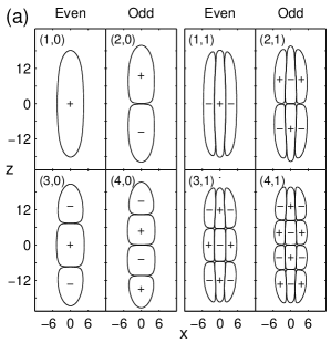
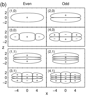
Figure 5: Highly anisotropic quasiparticle eigenstates in (a) prolate trap with $1/\lambda=7$ and (b) oblate trap with $\lambda=7$. The cases shown are the $f=1,2,3,4$ anomalous ($m=0$) family members with $n_{\mathrm{r}}=0$ and 1, respectively. The contour plots show contour lines only at $\pm 0.001$.

We have chosen to represent the $m=0$ modes, because the mode shapes are slightly simpler than the $m\neq 0$ modes (which differ only in having a zero along the $z$-axis). In highly anisotropic traps, the family shapes follow very well defined patterns, as we can see, and it is convenient to discuss the prolate and oblate cases separately.

Prolate case:

For the prolate case an increase in the principal family number $f$ simply adds an additional planar nodal surface perpendicular to the $z$-axis. Changing $n_{\mathrm{r}}$ from 0 to 1 adds a radial nodal surface which appears in this projection as two lines symmetric about, and almost parallel to the $z$-axis. The energy ordering of these modes is plotted in figure 6 (a) where we see that, for a given anisotropy, the energy ordering initially follows the family assignment $(f,0)$ with alternating even and odd modes.

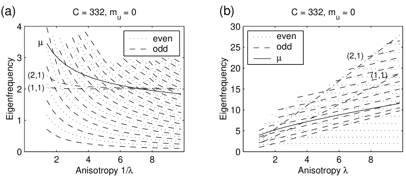
Figure 6: Frequency spectrum versus anisotropy of the low-lying $n_{\mathrm{r}}=0$ modes and the first two $n_{\mathrm{r}}=1$ modes ($m=0$) in (a) prolate, (b) oblate geometry. The even and odd modes with $n_{\mathrm{r}}=0$ are shown as dotted and dashed lines, respectively, and the $n_{r}=1$ modes as dashed-dotted lines. The solid line shows the condensate chemical potential $\mu$. The mode eigenfrequencies are measured relative to the condensate eigenvalue $\mu$.

This sequence is interrupted by the $(1,1)$ mode, at an energy near 2, where it has become more favourable to have a single radial nodal surface than many planar ones across the narrow dimension. We note that the higher the anisotropy (i.e. the larger $1/\lambda$) the more ($f,0$) modes fit in before the $(1,1)$ mode becomes favourable.

Oblate case:

Figure 5 (b) shows that in the oblate case it is natural to separate the sequences of even and odd modes. Then, successive members of each sequence (for fixed $n_{\mathrm{r}})$ are obtained by adding an additional cylindrical nodal surface about the $z$-axis, which in this projection appears as a pair of nodal lines parallel and symmetrically displaced with respect to the $z$-axis. Changing $n_{\mathrm{r}}$ from 0 to 1 adds again a radial nodal surface, which appears here as a pair of nodal lines parallel to and symmetrically placed about the $z=0$ plane.

In figure 6 (b), where the energies of the oblate modes are plotted as a function of the anisotropy $\lambda$, the distinction between the even and odd modes is clearly revealed. The odd modes are shifted as a group to higher energies than the even modes (reflecting the energy cost of the nodal surface through $z=0$), so that the energy ordering at a given anisotropy no longer simply alternates between even and odd. We see too that the even modes have essentially constant spacing except for very low $\lambda$, and the spacing of the odd modes, while compressed for low excitation numbers, becomes equal to the spacing of the even modes for higher excitation numbers. Once again, as for the prolate case, the higher the anisotropy the more $(f,0)$ modes fit in before the first $n_{\mathrm{r}}=1$ mode.

5.2 Comparison with harmonic oscillator solutions

For higher excitations the quasiparticle amplitude $v_{i}$ is negligible compared to $u_{i}$ and the BdG equations (3) reduce to the eigenvalue problem

$$[\hat{H}_{0}+2NU_{0}|\psi_{\mathrm{g}}(\mathbf{r})|^{2}-\mu]u_{i}(\mathbf{r})=\hbar\omega_{i}u_{i}(\mathbf{r}),$$ (8)

which has the form of a single particle equation [4, 12]. The presence of the condensate gives an effective potential that is broadly harmonic, but with a repulsive dimple in the middle, of height approximately $\mu$. At high excitations, the energy levels for equation (8) will be essentially those of the harmonic oscillator, while for mode energies comparable or less than $\mu,$ the presence of the dimple will shift the energy levels upwards, effectively compressing them.

If the condensate density is ignored in equation (8) the equation is simply that of the harmonic oscillator and is separable in cylindrical coordinates. The energy levels are given in units of $\hbar\omega_{\mathrm{r}}$ by

$$E=|m|+1+2n_{\rho}+2\lambda(n_{\mathrm{z}}+\frac{1}{4})\qquad$$ (even modes), (9)

$$E=|m|+1+2n_{\rho}+2\lambda(n_{\mathrm{z}}+\frac{3}{4})$$ (odd modes), (10)

where $n_{\rho}$ and $n_{\mathrm{z}}$ are the number of nodes in the $\rho$- and $z$-wave function respectively ($n_{\rho}=0,1,\ldots$, $n_{\mathrm{z}}=0,1,\ldots$). Equations (9) and (10) provide considerable insight into the behaviour of the solutions we have obtained from the full BdG equations.

In the prolate case, increasing $n_{\mathrm{z}}$ corresponds to increasing $f$ in the BdG solutions, while increasing $n_{\rho}$ corresponds to increasing $n_{\mathrm{r}}$ in the BdG solutions. For $\lambda<1$ it becomes energetically favourable to increase $n_{\mathrm{z}}$ rather than $n_{\rho}$, and we can fit roughly $1/\lambda$ nodes in the $z$-direction before it is energetically favourable to put a node in the $\rho$-direction. In figure 7 we show from calculations of the BdG equations the number $N^{(f,0)}$ of $(f,0)$ modes of lower energy than the first $n_{\mathrm{r}}=1$ mode and compare this qualitatively to the predictions from equations (9) and (10).

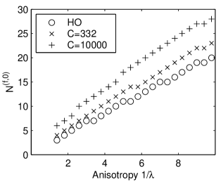
Figure 7: Comparison of energy ordering predictions of full BdG and harmonic oscillator solutions in a prolate trap. Plotted points show $N^{(f,0)}$, the number of $n_{\mathrm{r}}=0$ modes with energy lower than the $(1,1)$ mode. All modes are $m=0$.

We see that while there is relatively good agreement at $C=332$, the full BdG calculation predicts more $(f,0)$ modes to fit in, and the discrepancy increases at higher values of $C$. This is due to the fact that in the full equations the presence of the condensate causes the spacing of the lower levels (up to an energy of order $\mu$ above the condensate) to be compressed, and $\mu$ increases with $C$.

In the oblate case, the agreement between the harmonic oscillator solutions and the BdG solutions is much better. As explained in the previous section, it is useful to separate the even modes (where $n_{\mathrm{z}}$ corresponds to $2n_{\mathrm{r}}$, and $n_{\rho}$ to $(f-1)/2)$ and the odd modes (where $n_{\mathrm{z}}$ corresponds to $2n_{\mathrm{r}}+1$, and $n_{\rho}$ to $(f-2)/2)$. Since $\lambda>1$, it is now clear from equations (9) and (10) that increasing $n_{\mathrm{z}}$, i.e. increasing $n_{\mathrm{r}}$ in the BdG solutions, is more energetically costly than increasing $n_{\rho}$, which corresponds to increasing $f$. Figure 8 provides a quantitative comparison of the predictions of the harmonic oscillator solutions and the BdG solutions for the number of $(f,0)$ modes of lower energy than the first $n_{\mathrm{r}}=1$ mode.

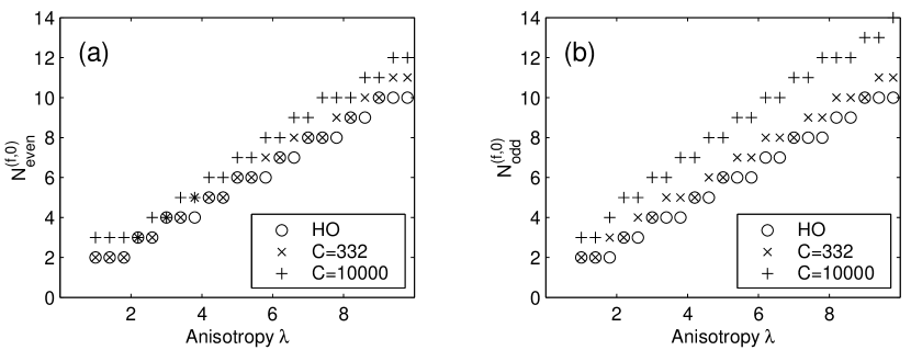
Figure 8: Comparison of energy ordering predictions of full BdG and harmonic oscillator solutions in the oblate case for (a) the number $N^{(f,0)}_{\mathrm{even}}$ of even $n_{\mathrm{r}}=0$ modes with energy lower than $(1,1)$ mode, (b) the number $N^{(f,0)}_{\mathrm{odd}}$ of odd modes with energy lower than the (2,1) mode. All modes are $m=0$.

We have separated the even and odd modes so that figure 8 (a) shows the number $N^{(f,0)}_{\mathrm{even}}$ of even modes with eigenfrequency lower than that of the (1,1) mode, while figure 8 (b) shows the number $N^{(f,0)}_{\mathrm{odd}}$ of odd modes with eigenfrequency lower than that of the (2,1) mode. The agreement is excellent for the $C=332$ case and still very good for the $C=10000$ case and is much better than for the prolate case of corresponding asymmetry, because the chemical potential $\mu$ lies lower relative to the eigenfrequencies in question, as can be seen in figure 6.

Finally, we remark that the magnetic quantum number $m$ simply gives an energy offset in equations (9) and (10), i.e. modes with a given number of nodes have higher energies for higher $m$. It is clear therefore, that the results discussed above for $m=0$ will also apply for $m\neq 0$. The energy offset by $m$ also explains that for a given family $(f,n_{\mathrm{r}})$ (i.e. a given number of nodes) the energy increases with increasing $m$ (see table 1).

6 Discussion

We have shown that the concept of mode families introduced by Hutchinson and Zaremba [5] can be systematically defined and extended to include all excitation modes of cylindrically symmetric anisotropic traps. The family assignment $(f$, $n_{\mathrm{r}})$ determines the topology of any mode with $m\neq 0,$ and the $m=0$ mode differs only in being non-zero on the symmetry axis. In the regime where the treatment of Fliesser et al [16] is valid, we can relate their quantum numbers $n$, $j$ to our family assignment numbers $f$ and $n_{\mathrm{r}}$ as follows:

$$f=n-2j+1,\qquad n_{\mathrm{r}}=j.$$ (11)

The similarity of shape of modes of the same family explains the similarity of frequency dependence on anisotropy for modes in a given family found by Hutchinson and Zaremba; changes in trap geometry affect every mode in the family in much the same way. We have also shown how the energy ordering of the quasiparticle excitations is related to their family shape and provided a simple model that explains the behaviour in terms of harmonic oscillator eigenstates.

References

References

- [1] Edwards M, Dodd R J, Clark C W and Burnett K 1996 J. Res. Natl. Inst. Stand. Techn. 101 553
- [2] Edwards M, Ruprecht P A, Burnett K, Dodd R J and Clark C W 1996 Phys. Rev. Lett. 77 1671
- [3] Ruprecht P A, Edwards M, Burnett K and Clark C W 1996 Phys. Rev. A 54 4178
- [4] You L, Hoston W and Lewenstein M 1997 Phys. Rev. A 55 R1581
- [5] Hutchinson D A W and Zaremba E 1998 Phys. Rev. A 57 1280
- [6] Cerboneschi E, Mannella R, Arimondo E and Salasnich L 1998 Phys. Lett. A 249 495
- [7] Fetter A L 1996 Phys. Rev. A 53 4245
- [8] Singh K G and Rokhsar D S 1996 Phys. Rev. Lett. 77 1667
- [9] Pérez-García V M, Michinel H, Cirac J I, Lewenstein M and Zoller P 1996 Phys. Rev. Lett. 77 5320
- [10] Sinha S 1997 Phys. Rev. A 55 4325
- [11] Stringari S 1996 Phys. Rev. Lett. 77 2360
- [12] Dalfovo F, Giorgini S, Guilleumas M, Pitaevskii L and Stringari S 1997 Phys. Rev. A 56 3840
- [13] Stringari S 1998 Phys. Rev. A 58 2385
- [14] Dalfovo F, Giorgini S, Pitaevskii L P and Stringari S 1999 Rev. Mod. Phys. 71 463
- [15] Öhberg P, Surkov E L, Tittonen I, Stenholm S, Wilkens M and Shlyapnikov G V 1997 Phys. Rev. A 56 R3346
- [16] Fliesser M, Csordás A, Szépfalusy P and Graham R 1997 Phys. Rev. A 56 R2533
- [17] Csordás A and Graham R 1999 Phys. Rev. A 59 1477
- [18] Braaten E and Pearson J 1999 Phys. Rev. Lett. 82 255
- [19] Jin D S, Ensher J R, Matthews M R, Wieman C E and Cornell E A 1996 Phys. Rev. Lett. 77 420
- [20] Jin D S, Matthews M R, Ensher J R, Wieman C E and Cornell E A 1997 Phys. Rev. Lett. 78 764
- [21] Mewes M-O, Andrews M R, van Druten N J, Kurn D M, Durfee D S, Townsend C G and Ketterle W 1996 Phys. Rev. Lett. 77 988
- [22] Stamper-Kurn D M, Miesner H-J, Inouye S, Andrews M R and Ketterle W 1998 Phys. Rev. Lett. 81 500
- [23] Onofrio R, Durfee D S, Raman C, Köhl M, Kuklewicz C E and Ketterle W 2000 Phys. Rev. Lett. 84 810
- [24] Fort C, Prevedelli M, Minardi F, Cataliotti F S, Ricci L, Tino G M and Inguscio M 2000 Europhys. Lett. 49 8
- [25] Fedichev P O and Shlyapnikov G V 1998 Phys. Rev. A 58 3146
- [26] Rusch M, Morgan S A, Hutchinson D A W and Burnett K 2000 Phys. Rev. Lett. 85 4844
- [27] Hutchinson D A W, Burnett K, Dodd R J, Morgan S A, Rusch M, Zaremba A, Proukakis N P, Edwards M and Clark C W 2000 J. Phys. B 33 3825
- [28] Giorgini S 2000 Phys. Rev. A 61 063615
- [29] Morgan S A, Choi S and Burnett K 1998 Phys. Rev. A 57 3818
- [30] Eisenhart L P 1948 Phys. Rev. 74 87
- [31] Dodd R J, Burnett K, Edwards M and Clark C W 1997 Phys. Rev. A 56 587