THERMODYNAMIC LIMIT FOR DIPOLAR MEDIA

Abstract

We prove existence of a shape and boundary condition independent thermodynamic limit for fluids and solids of identical particles with electric or magnetic dipole moments. Our result applies to fluids of hard core particles, to dipolar soft spheres and Stockmayer fluids, to disordered solid composites, and to regular crystal lattices. In addition to their permanent dipole moments, particles may further polarize each other. Classical and quantum models are treated. Shape independence depends on the reduction in free energy accomplished by domain formation, so our proof applies only in the case of zero applied field. Existence of a thermodynamic limit implies texture formation in spontaneously magnetized liquids and disordered solids analogous to domain formation in crystalline solids.

Keywords: Thermodynamic limit, Ferrofluid, Polar fluid, Dipole, Magnetism

I Introduction

Thermodynamics normally assumes a free energy density $F/V$ exists and is independent of system volume $V$ and shape. Verification of these properties is impeded by the explicit dependence of the partition function $Z=\exp{(-F/k_{B}T)}$ on these very quantities. Ruelle [1] and Fisher [2] proved the existence of thermodynamic limits for a large class of fluids and solids with interactions that fall off faster than $r^{-3}$ at large separation. For such systems the free energy contains a boundary independent, extensive (proportional to system volume) component and a boundary dependent, sub-extensive (less than proportional to system volume) remainder. Consequently, in the limit of infinite volume the free energy density approaches a finite, boundary independent, limit.

The interaction energy between dipoles falls off precisely as $r^{-3}$, seriously complicating the thermodynamic limit. Volume integrals of this interaction (required to calculate the total interaction energy ${\cal H}$) converge only conditionally because the power of $r$ with which the interaction decays matches the dimensionality of space. This paper considers systems with electric or magnetic dipole interactions. The electric and magnetic cases resemble each other closely. For convenience we carry out our discussion in the context of magnetism, then address electric analogues near the end of the paper.

Long-ranged dipole interactions may create shape dependent internal demagnetizing fields that increase the system free energy. Boundary conditions on the surfaces may influence the strength of these demagnetizing fields. The reduction in demagnetization energy when uniformly magnetized regions break into smaller domains is the key to the very existence of a thermodynamic limit in zero magnetic field. Griffiths [3] used the reversal of magnetization in a domain to prove existence of a thermodynamic limit independent of shape for dipolar lattices. We generalize that proof to include fluids and disordered solids. Certain conditions are required on the “residual interaction” ${\cal H}^{R}$, defined as the total interaction energy ${\cal H}$ minus the magnetic interaction energy ${\cal H}^{M}$. Our proof, like Griffiths’ original one, is valid only for zero applied field because of its reliance on magnetization reversal in domains.

The following section of our paper describes the origin of demagnetizing fields, leading to a shape dependent free energy in the presence of an applied field. In section II A we conjecture a simple functional form of the free energy, absorbing all shape dependence into a demagnetizing energy, implying a conventional thermodynamic limit for the remaining part of the free energy. Section II B describes how the system achieves a thermodynamic limit in zero field. Then, in section III, we outline the formal thermodynamic limit proof, which relies on upper and lower bounds on the free energy. We illustrate these bounds for stable and tempered systems in section III B. Section III C discusses the difficulty dipolar interactions cause due to their lack of tempering, and how that difficulty may be overcome. Section IV extends the proof to a variety of interesting specific models, starting with identical hard core particles, then treating dipolar soft spheres, the Stockmayer fluid and polarizable particles. We treat both classical and quantum versions of all these models. Section V addresses the analogous problems for electric dipoles. Finally, in section VI we summarize our results, discuss some observations about the implications of a thermodynamic limit for spontaneously polarized liquids, and conclude with some interesting dipolar systems which lack a thermodynamic limit.

II Demagnetizing fields

Long range dipole interactions create demagnetizing fields that cause the shape and boundary condition dependence of free energy in the presence of an applied field. In zero applied field the demagnetizing field must be handled with care to prove the shape and boundary condition independence of free energy. This section describes qualitatively why materials lack a shape independent thermodynamic limit in an applied field, and how the limit is restored in the absence of applied fields. We conjecture a modified form of thermodynamic limit that may hold in an applied field, with all the shape dependence restricted to an effective internal field plus an explicit demagnetizing energy term.

Volume and surface distributions of magnetic poles cause demagnetizing fields. Consider a sample of magnetic material contained in a region of space of volume $V$. Let ${\bf M}({\bf r})$ be the spatially varying magnetization in the sample. Poles arise at surfaces wherever the magnetization has a component normal to the surface $S$, as indicated in figures 1a and 1b. A magnetization with non-zero divergence produces a charge density in the bulk. The demagnetizing field takes the form

$${\bf H}_{D}({\bf r})=\int_{S}d^{2}{\bf r^{\prime}}~{}({\bf M}({\bf r^{\prime}})\cdot{\bf\hat{n}}({\bf r^{\prime}})){{\bf r-r^{\prime}}\over|{\bf r-r^{\prime}}|^{3}}-\int_{V}d^{3}{\bf r^{\prime}}~{}({\nabla}^{\prime}\cdot{\bf M}({\bf r^{\prime}})){{\bf r-r^{\prime}}\over|{\bf r-r^{\prime}}|^{3}}$$ (1)

where ${\bf{\hat{n}}}({\bf r^{\prime}})$ is the outward normal at any point on the surface. The spatial arrangement of surface charges depends on sample shape, and the divergence of ${\bf M}({\bf r})$ in the interior depends on the magnetization texture, so ${\bf H}_{D}({\bf r})$ is a function of sample shape and magnetization texture. The demagnetizing energy [4]

$$E_{D}=-{1\over{2}}\int d^{3}{\bf r}~{}{\bf H}_{D}({\bf r})\cdot{\bf M}({\bf r})={1\over{8\pi}}\int d^{3}{\bf r}~{}|{\bf H}_{D}({\bf r})|^{2}\geq 0$$ (2)

depends explicitly on the shape and magnetization texture of the system through the demagnetizing field ${\bf H}_{D}({\bf r})$.

In the special case of magnetization uniform throughout the sample, the demagnetizing field ${\bf H}_{D}({\bf r})$ comes only from the surface, because the divergence term in equation (1) vanishes. However, ${\bf H}_{D}({\bf r})$ does not vanish as volume increases at fixed shape. This is because the $1/r^{2}$ fall-off of the field from each surface charge is exactly offset by the $r^{2}$ growth of surface area, and hence the number of surface charges. As a result, ${\bf H}_{D}({\bf r})$ is independent of the volume and the demagnetizing energy $E_{D}$ is extensive.

For the special case of a uniformly magnetized ellipsoid, ${\bf H}_{D}$ is constant within the ellipsoid and equals

$${\bf H}_{D}=-4\pi{\bf D}\cdot{\bf M},$$ (3)

where the tensor ${\bf D}$ is the demagnetizing factor of the ellipsoid [4]. ${\bf D}$ is non-negative definite, and its trace equals 1. When the magnetization lies along a principal axis of the ellipsoid, ${\bf D}$ is simply replaced by one of its eigenvalues $0\leq D\leq 1$. For a magnetization parallel to a highly elongated needle shape, the demagnetizing factor $D=0$ because the surface poles appear only on the tips which are small and far removed from the bulk. Another special limit is that of magnetization normal to a flat pancake shape. This yields the maximum demagnetizing effect, since the surface poles appear on a large surface close to the bulk, so $D=1$ in this case.

A Shape dependence in a field

When a system is placed in an external field ${\bf H}_{0}$, surface poles arise because the internal magnetization tends to align with the applied field. There are two important contributions to the resulting shape dependence of the free energy. One is the explicit shape dependent energy (2), the other is due to the shape dependence of the internal field

$${\bf H}={\bf~{}H}_{0}+{\bf H}_{D}.$$ (4)

For highly elongated sample shapes, in the absence of demagnetizing effects, we expect a thermodynamic limit for the free energy. Define $f_{int}({\bf H}_{0})$ as the free energy per unit volume of a system in the limit as total volume $V\rightarrow\infty$. The limit must be taken within ellipsoidal shapes for which the length parallel to the field ${\bf H}_{0}$ grows faster than the orthogonal directions. Because there are no demagnetizing effects present, we call this free energy density the intrinsic free energy density in a field.

For more general shapes ${\bf H}_{D}$ is non-zero, and may vary in space. We conjecture that the shape dependent free energy $F_{shape}$ may be expressed in terms of the intrinsic free energy density as

$$F_{shape}({\bf H}_{0})=\int d^{3}{\bf r}~{}f_{int}({\bf H}({\bf r}))~{}+~{}E_{D}$$ (5)

up to corrections that grow less rapidly than the volume. Equation (4) gives the internal field H and equation (2) gives $E_{D}$.

Shape dependence of the free energy implies shape dependence of the measured paramagnetic susceptibility. Assume that the magnetization ${\bf M}$ is related to the internal field ${\bf H}$ by an intrinsic (volume and shape independent) linear susceptibility $\chi_{int}$ according to

$${\bf M}=\chi_{int}{\bf H}.$$ (6)

Consider applying an external field ${\bf H}_{0}$ parallel to a principal axis of an ellipsoidal sample. Because of the demagnetizing effect, the internal field H is weaker than the applied field. Eliminating ${\bf H}_{D}$ and ${\bf H}$ between equations (3), (4), and (6) yields the shape dependent measured susceptibility

$${\bf M}=\chi_{shape}~{}{\bf H}_{0}$$ (7)

where

$$\chi_{shape}={\chi_{int}\over{1+4\pi D\chi_{int}}}.$$ (8)

Note that the measured $\chi_{shape}$ has a maximum value equal to $\chi_{int}$ when ${\bf H}_{0}$ is parallel to the long axis of a highly prolate needle-shaped ellipsoid. For any other geometry the demagnetizing effect reduces the measured susceptibility.

B Shape independence in zero field

Now consider a ferromagnetic material in zero applied field. If the magnetization were constant (Fig. 1a), surface poles would create shape dependent demagnetizing fields and raise the energy as described in equation (2). A uniformly magnetized body lacks a shape independent thermodynamic limit!

Alternative magnetization configurations reduce the demagnetizing energy. One possibility (Fig. 1b) reverses magnetization in subregions so that the fields from surface poles tend to cancel. Another possibility (Fig. 1c) rotates the magnetization so that it is always tangent to the surface. In each case, the reduction in energy is proportional to the system volume $L^{3}$, where $L$ is a typical linear dimension. The energy increase arising at a sharp domain wall (Fig. 1b) should be proportional to the domain wall area $L^{2}$. The energy of a vortex line (Fig. 1c) should be proportional to $L\log(L/a)$, with $a$ related to the vortex core size. The magnetization texture may avoid a vortex by escaping into the the third dimension [5] near the core. Such textures contain either surface poles [6] or point defects [7]. For sufficiently large systems, the extensive $L^{3}$ reduction in the demagnetizing energy dominates the sub-extensive defect energies, and domain wall, vortex, surface pole or point defect formation is favored in that it lowers the free energy.

As we take the $V$ going to infinity limit, the demagnetizing energy density $E_{D}/V$ approaches zero for the most favorable magnetization, i.e., the one which minimizes the energy. Such a magnetization permits a shape independent thermodynamic limit for a ferromagnet. The free energy density for an arbitrary shape with its nonuniform equilibrium magnetization texture equals the free energy density of a highly elongated needle-shaped ellipsoid with uniform magnetization parallel to the long axis, because $D$ tends to zero for the needle shape. When calculating magnetic energies or free energies it may be convenient to impose the needle-shape and assume uniform polarization. Alternatively, “tin foil” boundary conditions [8] may be used to neutralize the surface poles.

Why is zero applied magnetic field essential for a thermodynamic limit? In an applied magnetic field the energy cost for flipping a domain becomes proportional to the domain volume (and grows proportionally to $L^{3}$) rather than the smaller domain wall, vortex or other defect energy. The most favorable magnetization texture now has a demagnetizing field, and the free energy re-acquires a shape dependence.

The above discussion explains how domain formation removes the demagnetizing energy density $E_{D}/V$, permitting a shape independent free energy for zero field ferromagnets. This argument does not apply to the zero field susceptibility of a paramagnet. The shape dependent susceptibility $\chi_{shape}$ governs fluctuations in the average magnetization of the entire sample. When this average fluctuates from zero, demagnetizing fields increase the free energy and oppose the fluctuation. Reduced fluctuations imply a reduced susceptibility that depends explicitly on shape through equation (8).

Still, we expect shape independent values of magnetic permeability $\mu=1+4\pi\chi_{int}$ (or dielectric constant $\epsilon$ in the case of electric polarizability). This can be understood by expressing the permeability in terms of spatial integrals of correlation functions [9, 10]. These correlation functions contain short-ranged, shape independent, components, and long-ranged, shape dependent components. The permeability depends only on the short-ranged, shape independent, part of the correlation functions.

III Proof of the Thermodynamic Limit

This section explains how we prove thermodynamic limits. First, we state required bounds on the free energy and explain how these bounds are used to prove the existence of a thermodynamic limit. Then, we show how to prove the necessary bounds on the free energy for classical systems which are stable and tempered. These sections are rather brief and formal, and simply review methods introduced previously [1, 2]. Then, in section III C we show how to treat systems which include unstable and non-tempered dipole interactions.

A Conditions on the Free Energy

Consider an $N$ particle system contained in a region ${\cal R}$ of volume $V$. Taking the thermodynamic limit for the free energy means constructing a sequence of sufficiently regular regions [2], with increasing volume, so that the number of particles $N$ divided by $V$ approaches a definite value $\rho$ as the volume $V$ tends to infinity. A limit is said to exist for the free energy density if the free energy $F$ divided by the system volume $V$ approaches a limiting value $f$ as the volume tends to infinity. The requirement of regularity [2] prevents the regions ${\cal R}$ from getting too thin or constricted. We also introduce a model-dependent density $\rho_{c}$ that ensures the particles can fit into the available volume when $N/V$ is less than $\rho_{c}$ for sufficiently large finite $N$.

Two conditions on $F$ suffice to prove the thermodynamic limit.

1) The free energy $F$ should satisfy the lower bound

$$F\geq Vf_{L}(N/V)$$ (9)

for $N/V<\rho_{c}$ where $f_{L}(\rho)$ is some finite valued function.

2) Consider a system composed of two subsystems, $1$ and $2$, containing $N_{1}$ and $N_{2}$ particles, respectively. The particles in subsystem $1$ are confined in a region ${\cal R}_{1}$ with volume $V_{1}$ and those in subsystem $2$ are confined in a region ${\cal R}_{2}$ with volume $V_{2}$. The two regions ${\cal R}_{1}$ and ${\cal R}_{2}$ are separated by a distance of at least $d$ from each other. Provided that $d\geq d_{0}$, for some fixed distance $d_{0}$, the free energy of the system should satisfy an upper bound

$$F\leq F_{1}+F_{2}+\Delta_{12},$$ (10)

where $F_{1}$ and $F_{2}$ are the free energies of subsystems $1$ and $2$ in isolation and [11]

$$\Delta_{12}\equiv(N_{1}+N_{2})^{2}\omega_{B}/d^{3+\epsilon},$$ (11)

with constants $\omega_{B}<\infty$ and $\epsilon>0$.

These bounds suffice for proving the existence and shape independence of the thermodynamic limit. Break an arbitrarily shaped system into many smaller subsystems. The upper bound (10) bounds the total free energy in terms of the subsystem free energies. Because the upper bound applies regardless of the relative positions of the subsystems, provided $d\geq d_{0}$, the original system shape does not enter this bound on total free energy. The lower bound (9) guarantees that the free energy density $F/V$ reaches a finite limit as the total volume $V~{}\rightarrow~{}\infty$ with $N/V~{}\rightarrow~{}\rho$. Because Fisher [2] explains this method in great generality, we need not reproduce his effort here.

B Classical Stable and Tempered Systems

The free energy of a classical system of $N$ identical particles in a volume $V$ is $F=-k_{B}T\log{Z}$, where $Z$ is the partition function

$$Z={{1}\over{\Omega^{N}N!}}\int_{V}\prod_{i=1}^{N}d^{3}{\bf r}_{i}d\Omega_{i}e^{-{\cal H}/k_{B}T}.$$ (12)

The energy ${\cal H}$ is a function of particle center of mass positions ${\bf r}_{i}$, and internal coordinates $\Omega_{i}$. In the expression for $Z$, $\Omega$ is the integral of $d\Omega_{i}$ over all its possible values. Internal coordinates depend on the type of particle and may include orientation of the particle and direction of magnetization. For solids, particle center of mass positions and particle orientations are fixed, and the principal remaining variable is direction of magnetization.

We distinguish between two types of particle: superparamagnetic particles [12], for which the direction of magnetization rotates independently of the particle axes; normal particles, for which the direction of magnetization is fixed relative to the particle axes. For normal particles, we do not include direction of magnetization as an independent internal variable, because it is a function of particle orientation. In practice, superparamagnetic particles exhibit a “blocking temperature” below which the direction of magnetization becomes locked to the particle axes, and the particles become normal. In the specific models discussed below, we assume we are below the blocking temperature except where we explicitly invoke superparamagnetism.

Note the explicit dependence of $Z$ on the system shape through the limits of integration for the ${\bf r}_{i}$ in equation (12). The free energy $F$ inherits this shape dependence. The conditions on $F$ stated in section III A guarantee that the shape dependence is contained entirely in a sub-extensive term. Achieving the desired lower and upper bounds on free energy depends on properties of the interaction energy ${\cal H}$. This section describes sufficient conditions to prove each bound.

The lower bound (9) holds for potentials that are stable in the sense that

$${\cal H}\geq-N\omega_{A}$$ (13)

with $\omega_{A}<\infty$ a constant. Just substitute the lower bound (13) for ${\cal H}$ into the partition function (12) to obtain the lower bound (9) on $F$, with the function

$$f_{L}(\rho)=\rho k_{B}T\log{\rho}-\rho\omega_{A}.$$ (14)

To prove the upper bound (10), consider the interaction of two subsystems separated by distance $d$ as described in section III A. Write the total energy ${\cal H}$ in the form

$${\cal H}\equiv{\cal H}_{1}+{\cal H}_{2}+{\cal H}_{12},$$ (15)

where ${\cal H}_{1}$ and ${\cal H}_{2}$ denote the energies of each system by itself, and ${\cal H}_{12}$ is the interaction energy between the two subsystems. The upper bound holds if the interaction ${\cal H}_{12}$ satisfies the weak tempering condition [11]

$${\cal H}_{12}\leq\Delta_{12}$$ (16)

with $\Delta_{12}$ as defined in equation (11), for $d$ larger than some constant $d_{0}$. Substitute $\Delta_{12}$ for ${\cal H}_{12}$ in the total interaction energy (15) and evaluate the partition function (12) to derive the upper bound (10) on $F$.

C Dipolar Systems

The remainder of this paper considers systems whose Hamiltonians include dipolar interactions in addition to stable, tempered interactions of the type described above. The dipole interaction, by itself, is neither stable nor tempered. In this section we explain how additional repulsive interactions may stabilize the system, and how the upper bound (10) may be proven despite the lack of tempering. The ideas introduced here are applied to a wide variety of specific models in section IV.

Split the interaction energy ${\cal H}$ into two components:

$${\cal H}={\cal H}^{M}+{\cal H}^{R}.$$ (17)

The non-magnetic part of the interaction, ${\cal H}^{R}$, we call the residual interaction. The magnetic interaction between the $N$ particles takes the form [4]

$${\cal H}^{M}=\sum_{i<j=1}^{N}\int_{v_{i}}d^{3}{\bf r}~{}\int_{v_{j}}d^{3}{\bf r}^{\prime}{\biggl{\{}}{{\bf M}({\bf r})\cdot{\bf M}({\bf r}^{\prime})\over|{\bf r-r^{\prime}}|^{3}}-{3({\bf M}({\bf r})\cdot({{\bf r-r^{\prime}}}))~{}({\bf M}({\bf r^{\prime}})\cdot({{\bf r-r^{\prime}}}))\over|{\bf r-r^{\prime}}|^{5}}{\biggl{\}}},$$ (18)

where $v_{i}$ and $v_{j}$ are the regions of space occupied by the magnetic material of particle $i$ and $j$. The magnetization distribution of the $i^{th}$ particle is ${\bf M}({\bf r})$ for ${\bf r}$ inside $v_{i}$, and for the $j^{th}$ particle is ${\bf M}({\bf r^{\prime}})$ for ${\bf r^{\prime}}$ inside $v_{j}$. Implicitly, ${\cal H}^{M}$ depends on the particle center of mass positions and the particle orientations through $v_{i}$ and $v_{j}$, the regions of space occupied by the particles. For superparamagnetic particles, the direction of magnetization is an internal coordinate for each particle, while for normal particles, the magnetization is determined by the particle orientation. Thus, ${\cal H}^{M}$ is a function of particle positions $\{{\bf r}_{i}\}$ and internal coordinates $\{\Omega_{i}\}$.

For the moment we consider only permanent magnetization (polarizable particles are discussed in section IV C), and we assume the magnetized volumes of the particles are non-overlapping. The $1/r^{3}$ dependence of the magnetic interaction ${\cal H}^{M}$ violates tempering because of its slow decay at long range, and risks violating stability because of its divergence at short range.

We demand stability of the total interaction ${\cal H}$ to enforce the lower bound (9) on the free energy. Because of the diverging short-range magnetic attraction, we need residual interactions that are sufficiently repulsive at short range to overcome the magnetic attraction. Hard-core particles, and soft-core particles with energies that diverge faster than $1/r^{3}$, satisfy this requirement, as we prove later in section IV.

To achieve the upper bound (10) on the free energy we demand that the residual interaction ${\cal H}^{R}$ be tempered and we exploit symmetries (if present) to handle the non-tempered magnetic interaction ${\cal H}^{M}$. Our strategy limits our proof to models possessing the required symmetries and tempering of residual interactions. Models lacking these characteristics may still possess a thermodynamic limit even though we cannot prove it. The symmetries we require are broken by applied magnetic fields.

Consider two subsystems such that the $N_{1}$ particles in region ${\cal R}_{1}$ are separated by at least a distance $d\geq d_{0}>0$ from the $N_{2}$ particles in region ${\cal R}_{2}$. Let ${\cal H}_{1}$ and ${\cal H}_{2}$ be their respective Hamiltonians. Define the interaction energy between the two subsystems by

$${\cal H}_{12}\equiv{\cal H}-{\cal H}_{1}-{\cal H}_{2}={\cal H}_{12}^{M}+{\cal H}_{12}^{R}.$$ (19)

Let $F(\lambda)$ be the free energy of the combined system when the Hamiltonian is ${\cal H}_{1}+{\cal H}_{2}$ plus a scaled interaction $\lambda{\cal H}_{12}$. Because $F(\lambda)$ is a concave function (that is, $F^{\prime\prime}(\lambda)\leq 0$), it is bounded above by

$$F(\lambda)\leq F(0)+\lambda F^{\prime}(0),$$ (20)

where the right side is a line tangent to the graph of $F(\lambda)$ at $\lambda=0$; here $F^{\prime}(\lambda)$ and $F^{\prime\prime}(\lambda)$ are the first and second derivatives. As a consequence, the free energy $F(1)$ of the fully interacting system satisfies the Gibbs inequality [13]

$$F(1)\leq F(0)+\langle{\cal H}_{12}^{M}+{\cal H}_{12}^{R}\rangle_{\lambda=0},$$ (21)

where $F(0)=F_{1}+F_{2}$ is the free energy of the non-interacting subsystems, and the classical ensemble average of any quantity ${\cal Q}$ takes the form

$$\langle{\cal Q}\rangle_{\lambda=0}={{1}\over{\Omega^{N_{1}+N_{2}}N_{1}!N_{2}!Z_{1}Z_{2}}}\int_{V_{1}}\prod_{i=1}^{N_{1}}d^{3}{\bf r}_{i}d\Omega_{i}\int_{V_{2}}\prod_{j=1}^{N_{2}}d^{3}{\bf r}_{j}d\Omega_{j}{\cal Q}e^{-({\cal H}_{1}+{\cal H}_{2})/k_{B}T}.$$ (22)

Because the residual interaction ${\cal H}^{R}$ is tempered, therefore ${\cal H}_{12}^{R}\leq\Delta_{12}$. Its ensemble average, likewise, is bounded above:

$$\langle{\cal H}_{12}^{R}\rangle_{\lambda=0}\leq\Delta_{12}.$$ (23)

We will show that

$$\langle~{}{\cal H}_{12}^{M}~{}\rangle_{\lambda=0}=0.$$ (24)

Combining the bound (21) with the ensemble averages (23) and (24) proves the upper bound (10) on the fully interacting free energy $F(1)$.

To establish (24) we employ what we call a $\theta$ operator, a map of the coordinates of a system onto themselves in a one-to-one manner satisfying the following conditions. It leaves the center of mass position ${\bf r}_{i}$ of each particle unchanged, it maps the internal coordinates $\Omega_{i}$ onto themselves in a way which leaves the integration measure $\prod_{i=1}d\Omega_{i}$ unchanged, and it leaves the Hamiltonian ${\cal H}$ invariant. In addition, when a system consists of two subsystems and $\theta$ is applied to one but not the other, it reverses the sign of the magnetic interaction ${\cal H}_{12}^{M}$ between them. Specific models may or may not possess such an operator. When a system is stable and possesses a $\theta$ operator, we can obtain the desired upper and lower bounds on $F$ to prove a thermodynamic limit.

If a $\theta$ operator exists, it can be used to establish (24) in the following way. Set ${\cal Q}={\cal H}_{12}^{M}$ in (22), and consider the change of variables produced by applying the $\theta$ operator to subsystem $1$ but not subsystem $2$. This change preserves the integration measure, but reverses the sign of the integrand, since ${\cal H}_{1}$ and ${\cal H}_{2}$ are unaltered, but ${\cal H}_{12}^{M}$ changes sign. Consequently, the integral is equal to its negative, so it is zero.

IV Models

Section III introduced a general strategy for proving thermodynamic limits of permanently magnetized classical particles. The following section applies that strategy to a variety of models. We start with identical hard core particles, then treat dipolar soft spheres such as Stockmayer fluids. We then modify the proof to cover polarizable particles, and then treat quantum systems. Depending on the particular system, the greater challenge may lie in demonstrating the lower, or the upper, bound on $F$.

A Identical hard core particles

Consider a collection of $N$ identical, uniformly magnetized, hard core normal particles of volume $v$, and fully contained within a region of space ${\cal R}$ of volume $V$. The magnetization ${\bf M}({\bf r})$ is constant in magnitude for ${\bf r}$ in volume $v_{i}$ of particle $i$ and vanishes when ${\bf r}$ is not inside a particle. Inside particle $i$ the direction of ${\bf M}({\bf r})={\bf M}_{i}$ depends on the orientation $\Omega_{i}$ of the particle. We require that the region ${\cal R}$ have a regular shape [2] and be large enough so that all particles fit inside the region without overlapping. Thus, we restrict the number of particles so that the packing fraction $\phi\equiv{Nv/V}$ is not too large. In particular, we assume a packing fraction $\phi^{*}>0$ exists for which particles may be packed with any $0\leq\phi\leq\phi^{*}$ into any sufficiently large and regular volume.

Write the Hamiltonian as

$${\cal H}={\cal H}^{M}+{\cal H}^{HC}.$$ (25)

The hard core interaction,

$${\cal H}^{HC}=\left\{\begin{array}[]{ll}0&\mbox{if no particles overlap,}\\ +\infty&\mbox{otherwise},\end{array}\right.$$ (26)

prevents any overlap between particles. For non-overlapping configurations the magnetic interaction ${\cal H}^{M}$ is as in (18). For the special case of hard core spheres the expression (18) reduces to the simpler form

$${\cal H}^{M}=\sum_{i<j=1}^{N}{\mbox{\boldmath$\mu$}_{i}\cdot\mbox{\boldmath$\mu$}_{j}-3(\mbox{\boldmath$\mu$}_{i}\cdot{\hat{\bf r}_{ij}})(\mbox{\boldmath$\mu$}_{j}\cdot{\hat{\bf r}_{ij}})\over{r_{ij}^{3}}}$$ (27)

where $\mbox{\boldmath$\mu$}_{i}$ and ${\bf r}_{i}$ are the dipole moment and position of the $i^{th}$ particle; $\mbox{\boldmath$\mu$}_{i}$ is the integral of ${\bf M}({\bf r})$ over the volume of the $i^{th}$ particle; ${\bf r}_{ij}={\bf r}_{i}-{\bf r}_{j}$, and ${\hat{\bf r}}_{ij}$ is the unit vector along ${\bf r}_{ij}$.

The hard core interaction (26) by itself provides an example of a stable and tempered interaction. Since ${\cal H}^{HC}\geq 0$, it obeys the stability condition (13) with $\omega_{A}=0$. Griffiths [3] proved the lower bound

$${\cal H}^{M}\geq-{N\mu^{2}\over{2R^{3}}},$$ (28)

for non-overlapping dipolar spheres with radius $R$, and dipole moment $\mu$, regardless of their positions and orientations. Because of the hard core repulsion (26) we achieve stability (13) with $\omega_{A}=\mu^{2}/2R^{3}$ for dipolar hard spheres (25). The lower bound on $F$ follows as discussed in section III B. We now generalize the proof of stability (13), and thus a lower bound on $F$, to particles of all shapes.

To prove stability we make use of the positivity of field energy. Adding the magnetic self energy of each particle to ${\cal H}^{M}$ gives the total energy of the whole system, considered as one magnetization distribution,

$${\cal H}^{T}={\cal H}^{M}+\sum_{i=1}^{N}E_{i}^{self}=-{1\over{2}}\int d^{3}{\bf r}~{}{\bf H}_{D}({\bf r})\cdot{\bf M}({\bf r}).$$ (29)

Here ${\bf H}_{D}({\bf r})$ is the field, due to all particles, defined in equation (1) and

$$E_{i}^{self}=-{{1}\over{2}}{\bf M}_{i}\cdot\int_{v_{i}}d^{3}{\bf r}~{}{\bf H}_{iD}({\bf r}),$$ (30)

where ${\bf H}_{iD}({\bf r})$ is the field from magnetization ${\bf M}_{i}$ of particle $i$ with volume $v_{i}$, obtained by substituting ${\bf M}_{i}$ for ${\bf M}({\bf r})$ in equation (1) and integrating over the surface and volume of particle $i$.

We use equation (29) to place a lower bound on ${\cal H}^{M}$ by a method similar to that of Griffiths [3]. For any magnetization distribution ${\bf M}({\bf r})$ and the field ${\bf H}_{D}({\bf r})$ caused by it

$$-{1\over{2}}\int d^{3}{\bf r}~{}{\bf H}_{D}({\bf r})\cdot{\bf M}({\bf r})={{1}\over{8\pi}}\int d^{3}{\bf r}~{}|{\bf H}_{D}({\bf r})|^{2}\geq 0.$$ (31)

Hence

$${\cal H}^{M}+\sum_{i=1}^{N}E_{i}^{self}\geq 0.$$ (32)

Brown [4] rewrites the self energy in (30) as

$$E_{i}^{self}=2\pi\sum_{k,l}D_{i}^{kl}M_{i}^{k}M_{i}^{l}~{}~{}v_{i},$$ (33)

where ${\bf D}_{i}$ is the demagnetizing tensor of an “equivalent ellipsoid”; it exists for a particle of any shape, and $k$ and $l$ index the components of ${\bf D}_{i}$ and ${\bf M}$. Since ${\bf D}_{i}$ is positive definite, with trace equal to 1,

$$E_{i}^{self}\leq 2\pi M^{2}v_{i}.$$ (34)

Since all particles are identical, the magnetic interaction satisfies the lower bound

$${\cal H}^{M}\geq-2\pi M^{2}Nv.$$ (35)

Thus we confirm stability (13). The lower bound (9) on the free energy follows with $\omega_{A}=2\pi M^{2}v$.

For proving an upper bound on the free energy, notice that the hard core interaction (26) is tempered, equation (16), with any $d_{0}>0$. We identify the hard core interaction (26) as a residual interaction ${\cal H}^{R}$. The key to our proof of an upper bound in Section III C was reversing the sign of the magnetic interaction energy ${{\cal H}}_{12}^{M}$, without changing ${\cal H}_{1}$, by applying an operator $\theta$ on subsystem $1$. For particles with permanent magnetization fixed relative to the particle, a rotation of each particle can reverse the direction of magnetization. Such a rotation keeps the residual interactions unchanged only if the particle shape has an axis of 2-fold symmetry perpendicular to its magnetization. Hence at least one operator $\theta$ exists, and our proof applies, for systems of identical particles with the required rotational symmetry in shape.

Some kinds of small particles, including many used in ferrofluids [14], exhibit superparamagnetism. Dipole moments rotate by Neel relaxation [15], or possibly quantum tunneling [16], without requiring rotation of the particle itself. To describe the superparamagnetic classical particles, one includes in $\Omega_{i}$, in addition to the Euler angles, a discrete variable $O_{i}=\pm 1$ specifying that the magnetization is parallel $(+1)$ or opposite $(-1)$ to a direction fixed in the particle, and $\int d\Omega_{i}$ includes a sum over $O_{i}$. The $\theta$ operator is the map $O_{i}\rightarrow-O_{i}$, applied to every particle. For a quantum particle, the corresponding operation is time reversal applied to the particle’s magnetization. In either case, the $\theta$ operator has the properties specified in section III C, so the argument given there shows that any system of hard core superparamagnetic particles, with any shape of particle, has a thermodynamic limit.

B Dipolar systems with central forces

Consider a system of particles interacting with Hamiltonian

$${\cal H}={\cal H}^{M}+{\cal H}^{(n)}+{\cal H}^{central}$$ (36)

where ${\cal H}^{M}$ is the point dipole interaction (27),

$${\cal H}^{(n)}=\sum_{i<j=1}^{N}{A\over{r_{ij}}^{n}}$$ (37)

is a repulsive interaction with $A>0$ and $n>3$, and ${\cal H}^{central}$ is any stable (13) and tempered (16) potential that is spherically symmetric. Define ${\cal H}^{(n)}+{\cal H}^{central}$ to be the residual interaction ${\cal H}^{R}$. The upper bound (10) follows exactly as in section III C because ${\cal H}^{(n)}$ and ${\cal H}^{central}$ are both tempered and rotationally invariant. The proof of a lower bound (9) for such systems is more complicated than for hard core particles because there is no minimum distance of separation between the point dipoles.

To prove stability (13) and hence a lower bound (9), it suffices to prove that ${\cal H}^{M}+{\cal H}^{(n)}$ is stable, since ${\cal H}^{central}$ is stable by assumption. Consider some configuration of a finite system of $N$ particles. Let $2R_{i}$ be the distance from the $i^{th}$ particle to its nearest neighbor. The magnetic interaction energy remains unchanged if each particle is replaced by a sphere of radius $R_{i}$ with uniform magnetization and the same dipole moment $\mu$. The self energy of such a sphere is $\mu^{2}/2R_{i}^{3}$. Since ${{\cal H}^{M}+(\mu^{2}/2)\sum_{i=1}^{N}R_{i}^{-3}\geq 0}$ by positivity of field energy (see discussion in section IV A), and ${\cal H}^{(n)}\geq(A/2)\sum_{i=1}^{N}({2R_{i}})^{-n}$, we write

$${\cal H}^{M}+{\cal H}^{(n)}\geq-\sum_{i=1}^{N}{{{\mu}^{2}}\over{2{R_{i}}^{3}}}+\sum_{i=1}^{N}{A\over{2({2R_{i}})^{n}}}.$$ (38)

Define a generalized mean

$$G(t)=({1\over N}\sum_{i=1}^{N}{1\over{R_{i}}^{t}})^{1\over t}.$$ (39)

Using the property that $G(t)$ increases monotonically for positive $t$ [17] we find

$${1\over N}\sum_{i=1}^{N}{1\over{R_{i}}^{n}}\geq({1\over N}\sum_{i=1}^{N}{1\over{R_{i}}^{3}})^{n/3},$$ (40)

for $n>3$. Combining equation (40) with equation (38) we write

$${\cal H}^{M}+{\cal H}^{(n)}\geq-N({{\mu}^{2}\over 2}X-{A\over 2^{n+1}}X^{n/3}),$$ (41)

where $X\equiv({1/N})\sum_{i=1}^{N}{R_{i}}^{-3}$. The bound (41) for ${\cal H}^{M}+{\cal H}^{(n)}$ has a minimum because $n>3$ and $A>0$. In particular

$${\cal H}^{M}+{\cal H}^{(n)}\geq-N[{\mu^{2}\over 2}({n-3\over n})({3~{}2^{n}\mu^{2}\over{nA}})^{3\over(n-3)}].$$ (42)

Our model (36) is therefore stable.

Let’s apply this general proof to some special cases. Our proof applies to generalized Lennard-Jones particles with dipole interactions. The Hamiltonian for such a system is

$${\cal H}={\cal H}^{M}+{\cal H}^{LJ},$$ (43)

where the Lennard-Jones potential is

$${\cal H}^{LJ}=\sum_{i<j}{B\over{r_{ij}}^{n}}-\sum_{i<j}{C\over{r_{ij}}^{m}}.$$ (44)

Ruelle [1] showed that generalized Lennard-Jones potentials with $B,C>0$ and $n>m>3$ are stable. To demonstrate stability including the dipole interaction, divide the repulsive term into two positive pieces, $B=A+B^{\prime}$. Attribute $B^{\prime}$ to a new (but still stable) Lennard-Jones potential and use the remainder $A$ to define the repulsive potential ${\cal H}^{(n)}$,

$${\cal H}={{\cal H}^{M}}+{{\cal H}^{(n)}}+{{\cal H}^{LJ^{\prime}}}.$$ (45)

The Hamiltonian in (45) is special case of our model (36). The Stockmayer fluid [19] is the case with $n=12,m=6$, and hence will also have a shape independent thermodynamic limit. Dipolar soft spheres [18] are the trivial case C=0 and ${\cal H}^{central}=0$.

C Polarizable Particles

Consider a system of identical hard core particles that contain permanent magnetic moments but are further linearly (i.e. proportionally to the local field) polarizable. The simplest model for such systems is the dipole-induced-dipole (DID) model [10, 20]. The model consists of spherical particles with a point dipole moment at the center, and with the induced polarization an additional point dipole moment of strength $\alpha{\bf H}$. This model lacks stability in general. For example, with two spherical particles of polarizability $\alpha$ and hard core radius $R$, stability is lost when

$${\alpha\over 4R^{3}}\geq 1.$$ (46)

The model fails because of its assumed induced point dipole. The point dipole applies rigorously only to an infinitesimal volume. However, the polarizability $\alpha$ necessarily vanishes in the limit of zero volume, due to the self-induced demagnetizing field. Finite size particles can have $\alpha\neq 0$. However, the DID model omits multipole moments due to the spatial variation of fields and magnetization inside the particles. Higher order multipole interactions between particles become important when the particles approach each other [22, 23], and are required for stability.

Consequently, we work with a more physically realistic model [20]. By incorporating the full magnetic interaction (dipole and higher moments) and the spatial variation of fields within a particle, our model satisfies stability in general. This model represents the polarizability of atoms and molecules more accurately than the DID model. Each particle has a permanent magnetization density which is constant in the interior of the particle, but whose direction is determined by the orientation of the particle. (For example, imagine that the particles are prolate ellipsoids with magnetization along the long axis.) The particles are “hard”, so that their volumes cannot overlap. Consequently, the permanent magnetization is a vector field ${\bf M}^{p}({\bf r})$, equal to zero unless ${\bf r}$ is inside some particle, where it takes on a value whose magnitude is independent of the particle but whose direction is tied to the particle’s orientation $\Omega$.

In addition, each particle contains linearly polarizable material giving rise to an induced magnetization

$${\bf M}^{i}({\bf r})=\mbox{\boldmath$\chi$}({\bf r})\cdot{\bf H}({\bf r}),$$ (47)

where ${\bf H}({\bf r})$ is the total magnetic field at ${\bf r}$, and the susceptibility tensor $\mbox{\boldmath$\chi$}({\bf r})$ is zero unless ${\bf r}$ is inside some particle, where its value is independent of ${\bf r}$ but tied to the orientation of the particle: that is the principal values of $\chi$ and the relationship of the principal axes of $\chi$ to the orientation of the particle is same for every particle.

The total magnetic field ${\bf H}({\bf r})$ in (47) is

$${\bf H}({\bf r})={\bf H}^{p}({\bf r})+{\bf H}^{i}({\bf r}),$$ (48)

where ${\bf H}^{p}({\bf r})$ is the field from permanent magnetization density ${\bf M}^{p}$, and is given by (1) with ${\bf M}$ set equal to ${\bf M}^{p}$, whereas ${\bf H}^{i}({\bf r})$ is due to the induced magnetization: in (1) set ${\bf M}$ equal to ${\bf M}^{i}$. Note that even an isolated particle will have an induced magnetization because the demagnetizing effect will give rise to a non-zero ${\bf H}^{p}$, and the total ${\bf H}$ inside the particle must be determined self-consistently, as it both induces a magnetization, (47), and is partly (${\bf H}^{i}$) determined by that magnetization.

Because of this requirement of consistency between total field and magnetization, the magnetic interaction of polarizable particles is a multi-body interaction, and is much more complicated than the pairwise multipole interactions of permanently magnetized particles discussed in section IV A. To write down the interaction energy ${\cal H}^{M}$ of a configuration of polarizable particles, it is convenient to calculate the work done assembling the configuration, starting with the particles well separated from each other at infinity. For any arrangement of particles, the total magnetic energy is

$${\cal H}^{T}={1\over{8\pi}}\int d^{3}{\bf r}~{}|{\bf H}^{p}|^{2}-{1\over{2}}\int d^{3}{\bf r}~{}{\bf H}^{p}\cdot{\bf M}^{i}.$$ (49)

The first term is the demagnetization energy (2) of the permanent magnetization distribution, and the second term represents the work done in introducing linearly polarizable material into this permanent field. Evaluating (49) for an isolated particle defines the self energy $E^{self}$ per particle. The difference

$${\cal H}^{M}\equiv{\cal H}^{T}-NE^{self}$$ (50)

equals the work done bringing initially isolated polarizable particles into interaction with each other.

The stability (13) and hence the lower bound (9) for this system follows from the positivity of field energy. Rewrite the magnetic energy in equation (49) as (see appendix A for details)

$${\cal H}^{T}={1\over{8\pi}}\int d^{3}{\bf r}~{}{\bf H}\cdot({\bf 1}+4\pi\mbox{\boldmath$\chi$})\cdot{\bf H}.$$ (51)

Since ${\bf 1}+4\pi\mbox{\boldmath$\chi$}$ is positive definite, ${\cal H}^{T}\geq 0$, hence

$${\cal H}^{M}\geq-NE^{self}.$$ (52)

The stability and lower bound then follow as in the case of identical hard core particles.

To prove the upper bound (10), consider two subsystems $1$ and $2$ separated by a distance $d\geq d_{0}>0$ as in section III A. Write the interaction Hamiltonian between these two subsystems as

$${{\cal H}_{12}^{M}}={\cal H}^{M}-{\cal H}_{1}^{M}-{\cal H}_{2}^{M},$$ (53)

where ${\cal H}_{1}^{M}$ and ${\cal H}_{2}^{M}$ are the magnetic interaction Hamiltonians for the subsystems by themselves; i.e. ${\cal H}_{1}^{M}$ is the energy of subsystem $1$ with subsystem $2$ placed infinitely far away. We show in appendix B that, for positive-definite $\chi$,

$${{\cal H}_{12}^{M}}={\cal O}_{12}^{M}+{\cal N}_{12}^{M},$$ (54)

where ${\cal O}_{12}^{M}$ is odd under reversal of the permanent magnetization of particles in subsystem $1$ by the $\theta$ operator, and ${\cal N}_{12}^{M}\leq 0$. Since ${\cal O}_{12}^{M}$ is odd, its ensemble average vanishes. Then

$$\langle{\cal H}_{12}^{M}\rangle_{\lambda=0}=\langle{\cal N}_{12}^{M}\rangle_{\lambda=0}\leq 0,$$ (55)

which is sufficient to prove the upper bound on $F$, as discussed in section III C.

D Quantum Systems

Our proofs extend to quantum systems. Consider a system of $N$ identical spin $S$ particles in volume $V$, which may obey Boltzmann, Fermi-Dirac or Bose-Einstein statistics. The Hamiltonian is

$${\cal H}={\cal K}+{\cal H}^{M}+{\cal H}^{EX}+{\cal H}^{R}.$$ (56)

Here ${\cal K}=\sum_{i=1}^{N}p_{i}^{2}/2m$ is the kinetic energy operator. The exchange interaction [21] is ${\cal H}^{EX}={{1}\over{2}}\sum_{ij}J(r_{ij}){\bf S}_{i}\cdot{\bf S}_{j}$, where ${\bf S}_{i}$ is the spin operator for particle $i$, $r_{ij}$ is the distance between particles $i$ and $j$, the couplings $J(r_{ij})$ are assumed to satisfy conditions consistent with stability, and the sum is over all $i\neq j$. The dipole interaction ${\cal H}^{M}$ is given by (27) with dipole moments $\mbox{\boldmath$\mu$}_{i}=g{\bf S}_{i}$. The residual interaction ${\cal H}^{R}$ may be any stable and tempered interaction that remains unchanged under simultaneous spin reversal of all particles, such as the hard core or central force interactions discussed in sections IV A and IV B. Implicit in our definition of the Hamiltonian is the confinement of particles in a region ${\cal R}$ of volume $V$ with hard wall boundary conditions. The partition function is

$$Z={{1}\over{C}}~{}{\rm Tr}~{}{\big{\{}}e^{-{\cal H}/k_{B}T}{\big{\}}}$$ (57)

where the trace Tr is carried out over states of appropriate symmetry with respect to interchange of particles. For Boltzmann particles $C=N!$ and for fermions and bosons $C=1$. The free energy $F$ is $-k_{B}T\log Z$.

The stability of ${\cal H}$, in the sense that its spectrum has a lower bound proportional to $N$, see (13), follows from the positivity of ${\cal K}$ (no negative eigenvalues) and the stability of ${\cal H}^{M}+{\cal H}^{EX}+{\cal H}^{R}$. Lower bounds on classical energies of the sort derived in sections IV A and IV B are easily extended to operator inequalities which demonstrate the stability of ${\cal H}^{M}+{\cal H}^{R}$. That this stability is preserved upon adding ${\cal H}^{EX}$ requires a suitable choice of $J(r)$. For example, in the case of hard core particles it suffices that $J(r)$ be bounded and decrease more rapidly than $r^{-3-\epsilon}$ for some $\epsilon>0$.

We now address the upper bound on the free energy. Write the Hamiltonian in the form

$${\cal H}={\cal H}_{1}+{\cal H}_{2}+{\cal H}_{12}$$ (58)

where ${\cal H}_{1}$ includes all terms in (56) (one particle, two-particle, etc.) involving only particles in the set ${\cal S}_{1}$ with labels $1,2,...,N_{1},$ ${\cal H}_{2}$ includes the terms involving only particles in the set ${\cal S}_{2}$ with labels $N_{1}+1,N_{1}+2,...,N_{1}+N_{2},$ and ${\cal H}_{12}$ all the remaining terms. The interaction energy ${\cal H}_{12}$ is a sum of magnetic dipole, exchange, and residual terms

$${\cal H}_{12}=H_{12}^{M}+{\cal H}_{12}^{EX}+{\cal H}_{12}^{R}.$$ (59)

It will also be convenient to define a scaled Hamiltonian

$${\cal H}(\lambda)={\cal H}_{1}+{\cal H}_{2}+\lambda{\cal H}_{12},~{}0\leq\lambda\leq 1.$$ (60)

To begin with, we assume that the $N_{1}$ particles with labels in ${\cal S}_{1}$ are confined to a region of space ${\cal R}_{1}\subset{\cal R}$ with volume $V_{1}$, while the $N_{2}=N-N_{1}$ particles with labels in ${\cal S}_{2}$ are confined to a region ${\cal R}_{2}\subset{\cal R}$ of volume $V_{2}$, and that the minimum separation of ${\cal R}_{1}$ and ${\cal R}_{2}$ is a distance $d\geq d_{0}$. Note that (in general) ${\cal R}$ is larger than ${\cal R}_{1}\cup{\cal R}_{2}$. The Hilbert space of this system is spanned by product states of the form

$$|\psi_{n,m}^{\cal U}\rangle=|\phi_{m}(1,...,N_{1})\rangle~{}|\chi_{n}(N_{1}+1,...,N_{1}+N_{2})\rangle.$$ (61)

where the integer arguments are particle labels. The $\{|\phi_{m}\rangle\}$ form a complete set of states for the $N_{1}$ particles in ${\cal R}_{1}$ with appropriate symmetry under interchange of particles and $\{|\chi_{n}\rangle\}$ is a similar set for the $N_{2}$ particles in ${\cal R}_{2}$. The product states (61) have no symmetry for the interchange of particles between the two sets ${\cal S}_{1}$ and ${\cal S}_{2}$, as indicated by the superscript ${\cal U}$. Due to this lack of symmetry the partition function is given by

$$Z_{N_{1},N_{2}}^{{\cal C},{\cal U}}={1\over D}{\rm Tr}~{}\{~{}e^{-{\cal H}/k_{B}T}\}$$ (62)

where $D=N_{1}!N_{2}!$ for Boltzmann particles and $D=1$ for fermions and bosons. If this partition function is evaluated using ${\cal H}$ with $\lambda=0$ in (60), $-k_{B}T$ times its logarithm is the sum $F_{1}+F_{2}$ of free energies for the separate systems of particles in regions ${\cal R}_{1}$ and ${\cal R}_{2}$, each evaluated as if the other region did not exist, since the interactions between the two sets of particles have been “turned off”.

An upper bound on the free energy $F$ of the full system of $N$ particles confined to region ${\cal R}$, in the form of the equation (10) is obtained through the following steps.

1) “Turn on” the interaction between the particles in regions ${\cal R}_{1}$ and ${\cal R}_{2}$ by letting $\lambda$ increase from $0$ to $1$. The resulting free energy is denoted by $F_{N_{1},N_{2}}^{{\cal C},{\cal U}}$. The superscript ${\cal C}$ indicates that particles are confined to regions ${\cal R}_{1}$ and ${\cal R}_{2}$.

2) Remove the constraint that only particles in set ${\cal S}_{1}$ are found in ${\cal R}_{1}$ and only those in set ${\cal S}_{2}$ are found in ${\cal R}_{2}$. Any particle may be anywhere in the union of ${\cal R}_{1}$ and ${\cal R}_{2}$, provided there are exactly $N_{1}$ particles in ${\cal R}_{1}$ and $N_{2}$ particles in ${\cal R}_{2}$. This involves introducing appropriately symmetrized wavefunctions.

3) Relax the constraint that precisely $N_{1}$ particles are in $R_{1}$ and $N_{2}$ in ${\cal R}_{2}$. We still require that there be a total of $N$ particles in the union of ${\cal R}_{1}$ and ${\cal R}_{2}$.

4) Relax the constraint that the particles lie in either ${\cal R}_{1}$ or ${\cal R}_{2}$ , so that all particles can be anywhere in the larger region ${\cal R}$.

Since steps 2, 3, and 4 do not require special attention to long range interactions, they are discussed in Appendix C. Basically, each time a constraint is relaxed the free energy decreases, except for step 2, where it remains constant. Thus the upper bound obtained for $F_{N_{1},N_{2}}^{{\cal C},{\cal U}}$ applies to $F$.

For step 1 we use the fact that $F_{N_{1},N_{2}}^{{\cal C},{\cal U}}$ is a concave function of $\lambda$, and therefore

$$F_{N_{1},N_{2}}^{{\cal C},{\cal U}}(1)\leq F_{N_{1},N_{2}}^{{\cal C},{\cal U}}(0)+(dF_{N_{1},N_{2}}^{{\cal C},{\cal U}}/d\lambda)_{\lambda=0},$$ (63)

which is known as the Bogoliubov inequality [13]. The first term on the right is $F_{1}+F_{2}$, and the second is

$$\langle{\cal H}_{12}\rangle_{\lambda=0}=\langle{\cal H}_{12}^{M}\rangle_{\lambda=0}+\langle{\cal H}_{12}^{EX}\rangle_{\lambda=0}+\langle{\cal H}_{12}^{R}\rangle_{\lambda=0},$$ (64)

where the averages are with respect to Boltzmann weights with $\lambda=0$. For example

$$\langle{\cal H}_{12}^{M}\rangle_{\lambda=0}={\rm Tr}~{}\{{\cal H}_{12}^{M}~{}e^{-({\cal H}_{1}+{\cal H}_{2})/k_{B}T}~{}\}/{\rm Tr}~{}\{e^{-({\cal H}_{1}+{\cal H}_{2})/k_{B}T}~{}\}.$$ (65)

The third term in (64) is bounded by the upper bound $\Delta_{12}$ on ${\cal H}_{12}^{R}$. The first and second terms vanish for the following reason. Let $\theta$ be the anti-unitary spin reversal operator which reverses all the spins of the particles in collection ${\cal S}_{1}$. It is a symmetry of ${\cal H}_{1}$, because ${\cal H}_{1}^{M}$ and ${\cal H}_{1}^{EX}$ involve products of two spin operators and ${\cal H}_{1}^{R}$ is, by assumption, invariant under the reversal of all spins. Consequently, if the $\{|\phi_{m}\rangle\}$ are the eigenstates of ${\cal H}_{1}$, the states $\theta|\phi_{m}\rangle=|\hat{\phi}_{m}\rangle$ are also eigenstates with the same eigenvalues. In evaluating the trace in the numerator of (65) we can employ a complete set $\{|\phi_{m}\rangle|\chi_{n}\rangle\}$, where the $\{|\chi_{n}\rangle\}$ are the eigenstates of ${\cal H}_{2}$, or, equivalently, $\{|{\hat{\phi}}_{m}\rangle|\chi_{n}\rangle\}$. However,

$$\langle\hat{\phi}_{m}|\langle{\chi}_{n}|{\cal H}_{12}^{M}|\hat{\phi}_{m}\rangle|\chi_{n}\rangle=-\langle\phi_{m}|\langle{\chi}_{n}|{\cal H}_{12}^{M}|\phi_{m}\rangle|\chi_{n}\rangle$$ (66)

because

$$\langle\hat{\phi}_{m}|{\bf S}_{i}|\hat{\phi}_{m}\rangle=-\langle\phi_{m}|{\bf S}_{i}|\phi_{m}\rangle$$ (67)

for $1\leq i\leq N_{1}$, and ${\cal H}_{12}^{M}$ is a sum of pairwise products of spin operators, one from the collection ${\cal S}_{1}$ and one from ${\cal S}_{2}$. Thus $\langle{\cal H}_{12}^{M}\rangle_{\lambda=0}$ is equal to its negative and vanishes. The same argument applies to $\langle{\cal H}_{12}^{EX}\rangle_{\lambda=0}$.

Consequently, after following the remaining steps 2, 3, and 4 contained in appendix C, we have a bound corresponding to (10) in the classical case. This bound together with that in (9), which (as already noted) follows from the stability of ${\cal H}$, completes the proof of the existence of a thermodynamic limit in the quantum case, see section III A.

It is possible to treat the translation degrees of freedom classically and the spin quantum mechanically. The proof of a thermodynamic limit for such a “semi quantum” model is similar to the “fully quantum” treatment. The averages of ${\cal H}_{12}^{M}$ and ${\cal H}_{12}^{EX}$ involve sums over all spin states and integrals over all particle positions. Using the spin reversal operator $\theta$, introduced earlier in this section, and doing the sums over all spin states first, one sees that the average values of ${\cal H}_{12}^{M}$ and ${\cal H}_{12}^{EX}$ vanish. The residual interactions ${\cal H}_{12}^{R}$ are bounded by $\Delta_{12}$, and therefore our proof goes through.

One may define another “semi quantum” model of classical spins and classical dipoles with center-of-mass motion of the particles treated quantum mechanically. The averages of ${\cal H}_{12}^{M}$ and ${\cal H}_{12}^{EX}$ contain integrals over all spin orientations and sums over all spatial wavefunctions in this case. The proof is similar to that of classical particles. Doing the integrals over particle spins first, gives zero for the average of ${\cal H}_{12}^{M}+{\cal H}_{12}^{EX}$, because they are both odd with respect to spin reversal. The sum over the spatial wavefunctions then yields the desired upper bound on $\langle{\cal H}_{12}\rangle_{\lambda=0}$ and our proof goes through. We can even include classical polarizability (section IV C) in such a model. In this case the average of ${\cal H}_{12}^{M}$ is non positive, and again we get the required upper bound (10) on the free energy.

V Electric Polarization

So far we phrased our discussion entirely in terms of magnetic interactions. However our proof applies to many electrically polarized or polarizable materials as well. Electric fields ${\bf E}$ and ${\bf D}$ fields satisfy the same Maxwell equations as magnetic fields ${\bf H}$ and ${\bf B}$, respectively, provided no free charges and currents are present. By replacing fields ${\bf H}$, ${\bf B}$ and magnetization ${\bf M}$ with fields ${\bf E}$, ${\bf D}$ and polarization ${\bf P}$, respectively, our proofs run exactly as for magnetic materials. We assume stability, tempering of the residual interactions, and the existence of a $\theta$ operator. Thus we prove the existence of a shape independent thermodynamic limit for the electric analogue of each of the classical models discussed in sections IV.

For ferroelectric identical hard core particles, use the Hamiltonian

$${\cal H}={\cal H}^{P}+{\cal H}^{HC}$$ (68)

where ${\cal H}^{P}$ is the electric interaction between particles. The proof follows section IV A with the replacement of fields discussed at the beginning of this section. For electric dipolar systems with central forces the interaction Hamiltonian is

$${\cal H}={\cal H}^{P}+{\cal H}^{(n)}+{\cal H}^{central}.$$ (69)

The proof goes through as in section IV B, with the existence of a shape independent thermodynamic limit for electric dipolar soft spheres and Stockmayer fluids as special cases. For electrically polarizable particles, ${\cal H}={\cal H}^{P}+{\cal H}^{HC}$ where ${\cal H}^{P}$, the electric interaction between polarizable particles, is defined analogously with ${\cal H}^{M}$ in equation (50). After the replacements of fields and magnetization discussed at the beginning of this section, the proof proceeds as in section IV C. Quantum models can be treated as discussed in section IV D.

Adding another layer of complexity, we may define models combining features of electric and magnetic models already discussed. The possible variations are too numerous to describe individually. We simply note here that stability including only magnetic or only electric interactions ensures stability with the two added together. Finding a $\theta$ operator may be more difficult. For example, a $180^{\circ}$ rotation axis must lie perpendicular to both ${\bf M}$ and ${\bf P}$.

For the crude dipolar particle models discussed above, the electric and magnetic problems are fully equivalent. For applications to realistic models of specific materials, however, it is generally harder to find a $\theta$ operator in the case of electric materials. The analogue of time reversal (which provides a $\theta$ operator for superparamagnetic particles) is charge conjugation. This has the undesirable effect of turning matter into antimatter! Without a $\theta$ operator we cannot apply our proof.

For an example of a model outside our proof, consider a fluid of H₂O molecules (water). Modeled as a dipolar hard sphere or a Stockmayer fluid the thermodynamic limit follows from our discussions above using rotation as the $\theta$ operator. Real H₂O molecules lack this rotational symmetry. For example, the TIPS 3 site model of water [24] places positive charges on the hydrogens and a negative charge on oxygen. Coulomb interactions between all intermolecular pairs of charges, and a Lennard-Jones interaction between the oxygen atoms, gives the interaction

$${\cal H}_{mn}=\sum_{ij}{q_{i}q_{j}\over r_{ij}}+{A\over r_{OO}^{12}}-{C\over r_{OO}^{6}},$$ (70)

between any two water molecules $m,n$, where $i$ and $j$ run over the charges $q_{i}$ and $q_{j}$, respectively, on molecule $m$ and $n$, $r_{ij}$ is the separation between charges and $r_{OO}$ is the separation between oxygen ions. For the above model there is no symmetry operation available which can reverse all the electric interactions while keeping the residual (Lennard-Jones) interactions unchanged. A $\theta$ operator therefore does not exist for this model and we cannot apply our proof. We suppose that our qualitative argument (section II B) demonstrating existence of a shape independent thermodynamic limit based on domain formation still holds, but for technical reasons we cannot prove it.

Yet another example is provided by models of ferroelectric materials with mobile charges. Charges transfer among dissimilar chemical elements, so no $\theta$ operator is likely to exist. Furthermore, the definition of polarization becomes ambiguous, depending on how the unit cell is defined in the case of a crystal [25], or on the surface charge for non-crystalline materials. The question of appropriate thermodynamic limits for model ferroelectrics with mobile charges remains under discussion [26].

For models containing only bound charges, our qualitative argument (section II B) suggests the equilibrium state has no depolarizing energy density. When the microscopic coulomb charges are taken into account, including the possibility of molecular dissociation and the Fermi statistics of the constituent particles, the problem falls into the class of materials for which Lieb [27] proved a thermodynamic limit. Free electric charges screen the $1/r$ Coulomb potential, restoring the thermodynamic limit.

VI Conclusions

We proved the existence and shape independence of the free energy density for a variety of dipolar systems. Three essential conditions were identified: stability, tempering of residual interactions, and the existence of a $\theta$ operator that commutes with ${{\cal H}}_{1}$, ${\cal H}_{2}$ and ${\cal H}_{12}^{R}$ while reversing the sign of ${\cal H}_{12}^{M}$. Our proof covers systems of identical hard core particles with uniform permanent magnetization. We also treat dipolar soft spheres and Stockmayer fluids, systems with magnetizable or polarizable material, and we consider electric as well as magnetic dipoles. Except for the case of super-paramagnetic particles, the existence of a $\theta$ operator requires symmetries such as a 2-fold axis of rotational symmetry perpendicular to the magnetization/polarization of each particle.

Having proven shape independence of the free energy we now consider some implications of the proof. For the systems covered by our proof, thermodynamic states and phase diagrams do not depend on size or shape [28]. Intrinsic thermodynamic quantities such as pressure and chemical potential are independent of sample shape and position within a sample. When calculating free energies of magnetized states, care must be taken to remove the depolarizing field if uniform magnetization is assumed. Failure to do so leads to either boundary-condition or shape dependence of thermodynamic properties [26, 28, 29, 30]. Two convenient ways to remove the demagnetizing fields are to study highly prolate ellipsoids or to use tin-foil boundary conditions [8].

Computer simulations [31] suggest dipolar fluids such as ferrofluids may spontaneously magnetize. Experiments on supercooled CoPd alloys [32] claim to observe a spontaneously magnetized metastable state. How then can we reconcile shape independence of the free energy with these reports of spontaneously polarized liquid states? Domains or textures must form, as in equilibrium solid ferromagnets. Liquids lack the crystalline anisotropy required to sustain a sharp domain wall (see Fig. 1b). De Gennes and Pincus [33] note, however, that domain wall thickness should be comparable to system dimensions in a magnetic liquid. We conclude that a spontaneously polarized liquid has a position dependent axis of polarization that rotates so as to lie tangent to the sample surface. Since vector fields tangent to the surface of simply connected volumes exhibit singularities (the “hairy billiard ball” problem), magnetized fluid droplets must contain defects in the magnetization field ${\bf M}$. Possible textures include line (Fig. 1c) or point defects (not shown). Away from such defects the magnitude of magnetization $|{\bf M}|$ is independent of position within the sample. In computer simulations a uniformly polarized state is observed because the Ewald summations [8] drop the surface pole energy (via “tin-foil” boundaries) and thus mimic an infinite, boundary-free, medium.

Our proof is valid only in zero applied field. The case of an applied field is still open. The free energy in a field depends on shape as outlined in section II. The free energy increase due to the demagnetizing field causes a droplet of paramagnetic liquid to elongate in an external field, minimizing its magnetic energy by reducing $D$ [34]. However, we conjecture the existence of an intrinsic thermodynamic energy, defined in equation (5) by subtracting the shape dependent demagnetizing energy from the full shape dependent free energy.

Finally, let’s consider some dipolar systems to which we are unable to apply our proof due to the lack of a $\theta$ operator. Particles with non-symmetric shapes and magnetization fixed with respect their body (Fig. 2a) provide an example. Each particle is a cube with protrusions (conical, hemispherical and cubic) on three faces and matching indentations on the opposite three faces. Each face of one particle fits exactly into the corresponding opposite face of another particle. Recall that we exploit symmetries of the Hamiltonian when applying a $\theta$ operator to the internal coordinates $\Omega_{i}$. The $\theta$ operator, if it exists, reverses the sign of ${\cal H}_{12}^{M}$ while leaving ${\cal H}_{1}$ invariant. Rotations are not a symmetry of the internal coordinates for these particles. There is no evident symmetry of the Hamiltonian which could be used as a $\theta$ operator.

When these particles are tightly packed (i.e. the limit of infinite pressure and hard cores), they align parallel to each other. ${\bf M}$ is uniform throughout space and therefore the thermodynamic limit does not exist. At finite pressure it is possible to accumulate enough free volume to insert domain walls, (Fig. 2b), so we expect that the thermodynamic limit does exist even though the conditions of our proof are not obeyed. That is, our conditions are sufficient but not in all cases necessary.

Another interesting example is provided by hydrogen absorption in metals [35]. Interstitial hydrogen creates elastic strain fields that fall off as $1/r^{3}$, and hence are referred to as dipoles. This is a rather confusing notation, since the angular dependence is actually a sum of a quadrupole and a monopole contribution. The monopole term is the trace of the strain tensor and governs lattice dilation. Provided the system remains coherent (the lattice structure is dislocation free), the monopole interactions are shape dependent, attractive and infinite ranged. The interactions reduce the energy but create no force. In the coherent state, the phase diagram for liquid-gas transitions of hydrogen in a metal depends on the shape of the metal [36].

The coherent state itself is a metastable state. The true equilibrium state is incoherent, with dislocations relaxing the lattice strain. If one allows for dislocations, the elastic interactions become short ranged and the thermodynamic limit is restored. The sample itself, however, may have disintegrated into a fine powder!

A Total magnetic energy for polarizable dipoles

We start with equation (51) for ${\cal H}^{T}$ and show that it equals equation (49). Use equations (47) for induced magnetization ${\bf M}^{i}$ and (48) defining the permanent and induced fields ${\bf H}^{p}$ and ${\bf H}^{i}$ to rewrite equation (51) as

$${\cal H}^{T}={1\over{8\pi}}\int d^{3}{\bf r}~{}|{\bf H}^{p}|^{2}+{1\over{8\pi}}\int d^{3}{\bf r}~{}|{\bf H}^{i}|^{2}+{1\over{4\pi}}\int d^{3}{\bf r}~{}{\bf H}^{p}\cdot{\bf H}^{i}$$ (A1)

$$+{1\over{2}}\int d^{3}{\bf r}~{}{\bf H}^{p}\cdot{\bf M}^{i}+{1\over{2}}\int d^{3}{\bf r}~{}{\bf H}^{i}\cdot{\bf M}^{i}$$ (A2)

For any two magnetization distributions ${\bf M}_{1}({\bf r})$, and ${\bf M}_{2}({\bf r})$ and the fields ${\bf H}_{1}({\bf r})$ and ${\bf H}_{2}({\bf r})$ caused by them respectively, the following identity holds [4]:

$${1\over{8\pi}}\int d^{3}{\bf r}~{}{\bf H}_{1}\cdot{\bf H}_{2}=-{1\over{2}}\int d^{3}{\bf r}~{}{\bf H}_{1}\cdot{\bf M}_{2}=-{1\over{2}}\int d^{3}{\bf r}~{}{\bf H}_{2}\cdot{\bf M}_{1}$$ (A3)

Since equation (A3) holds for any two arbitrary magnetization distributions, we set ${\bf M}_{1}={\bf M}_{2}$ equal to the induced magnetization ${\bf M}^{i}$. Then equation (A3) gives

$${1\over{8\pi}}\int d^{3}{\bf r}~{}|{\bf H}^{i}|^{2}=-{1\over{2}}\int d^{3}{\bf r}~{}{\bf H}^{i}\cdot{\bf M}^{i}.$$ (A4)

Similarly, setting ${\bf M}_{1}={\bf M}^{p}$ and ${\bf M}_{2}={\bf M}^{i}$ in equation (A3) gives

$${1\over{8\pi}}\int d^{3}{\bf r}~{}{\bf H}^{p}\cdot{\bf H}^{i}=-{1\over{2}}\int d^{3}{\bf r}~{}{\bf H}^{p}\cdot{\bf M}^{i}.$$ (A5)

Using equations (A4) and (A5) to simplify equation (A1) gives equation (49), proving equality of our expressions (49) and (51) for ${\cal H}^{T}$.

B Interaction energy between two subsystems of polarizable dipoles

Let ${\bf H}_{1}^{p}({\bf r})$ and ${\bf H}_{2}^{p}({\bf r})$ be the fields due to the permanent polarization in subsystems $1$ and $2$ located in non-overlapping regions ${\cal R}_{1}$ and ${\cal R}_{2}$. The induced magnetizations in the two subsystems can be written in the form

$${\bf M}_{1}^{i}({\bf r})={\bf M}_{1}^{s}({\bf r})+{\bf M}_{1}^{{}^{\prime}}({\bf r}),$$ (B1)

$${\bf M}_{2}^{i}({\bf r})={\bf M}_{2}^{s}({\bf r})+{\bf M}_{2}^{{}^{\prime}}({\bf r}),$$ (B2)

where ${\bf M}_{1}^{s}({\bf r})$ is the induced magnetization which would be present in subsystem $1$ were subsystem $2$ absent, and ${\bf M}_{2}^{s}({\bf r})$ that of subsystem $2$ were subsystem $1$ absent.

Using equations (49) for ${\cal H}^{T}$ and (50) for ${\cal H}^{M}$ to find the interaction Hamiltonians ${\cal H}_{1}^{M}$, ${\cal H}_{2}^{M}$ and ${\cal H}^{M}$ for the two subsystems and the whole system, respectively, we write the interaction energy in (53) as

$${{\cal H}_{12}^{M}}={1\over{4\pi}}\int d^{3}{\bf r}~{}{\bf H}_{1}^{p}\cdot{\bf H}_{2}^{p}-{1\over{2}}\int d^{3}{\bf r}~{}{\bf H}_{2}^{p}\cdot{\bf M}_{1}^{s}-{1\over{2}}\int d^{3}{\bf r}~{}{\bf H}_{1}^{p}\cdot{\bf M}_{2}^{s}$$ (B3)

$$-{1\over{2}}\int d^{3}{\bf r}~{}({\bf H}_{1}^{p}+{\bf H}_{2}^{p})\cdot{\bf M}_{1}^{{}^{\prime}}-{1\over{2}}\int d^{3}{\bf r}~{}({\bf H}_{1}^{p}+{\bf H}_{2}^{p})\cdot{\bf M}_{2}^{{}^{\prime}}.$$ (B4)

Break ${{\cal H}_{12}^{M}}$ into odd and non-positive components ${{\cal H}_{12}^{M}}={\cal O}_{12}^{M}+{\cal N}_{12}^{M}$, where

$${\cal O}_{12}^{M}={1\over{4\pi}}\int d^{3}{\bf r}~{}{\bf H}_{1}^{p}\cdot{\bf H}_{2}^{p}\\ -{1\over{2}}\int d^{3}{\bf r}~{}{\bf H}_{2}^{p}\cdot{\bf M}_{1}^{s}-{1\over{2}}\int d^{3}{\bf r}~{}{\bf H}_{1}^{p}\cdot{\bf M}_{2}^{s}$$ (B5)

is odd under reversal of the permanent magnetization of particles in subsystem $1$ by the $\theta$ operator, and

$${\cal N}_{12}^{M}=-{1\over{2}}\int d^{3}{\bf r}~{}({\bf H}_{1}^{p}+{\bf H}_{2}^{p})\cdot{\bf M}_{1}^{{}^{\prime}}-{1\over{2}}\int d^{3}{\bf r}~{}({\bf H}_{1}^{p}+{\bf H}_{2}^{p})\cdot{\bf M}_{2}^{{}^{\prime}}$$ (B6)

is non-positive as we now show. A theorem by Brown [4] states that for a paramagnetic polarizable material in an applied field, the unique induced magnetization ${\bf M}^{i}$ given by equation (47) minimizes the total magnetic energy. Applying that theorem to our system we observe that

$$-{1\over{2}}\int d^{3}{\bf r}~{}({\bf H}_{1}^{p}+{\bf H}_{2}^{p})\cdot{\bf M}_{1}^{i}-{1\over{2}}\int d^{3}{\bf r}~{}({\bf H}_{1}^{p}+{\bf H}_{2}^{p})\cdot{\bf M}_{2}^{i}\leq$$ (B7)

$$-{1\over{2}}\int d^{3}{\bf r}~{}({\bf H}_{1}^{p}+{\bf H}_{2}^{p})\cdot{\bf M}_{1}^{s}-{1\over{2}}\int d^{3}{\bf r}~{}({\bf H}_{1}^{p}+{\bf H}_{2}^{p})\cdot{\bf M}_{2}^{s}.$$ (B8)

because the interaction-induced magnetization ${\bf M}^{i}$ has lower energy than the isolated self-magnetization ${\bf M}^{s}$. Upon replacing ${\bf M}_{j}^{{}^{\prime}}$ in (B6), with ${\bf M}_{j}^{i}-{\bf M}_{j}^{s}$, (B1), one sees that (B7) implies that

$${\cal N}_{12}^{M}\leq 0.$$ (B9)

C Quantum Systems

Here are the details for steps 2, 3, and 4 in section IV D. For step 2 note that the formal Hamiltonian ${\cal H}(\lambda=1)$, defined in equation (60), is symmetrical under the interchange of any two particles, since the right side of (58) is simply a way of segregating terms in the sum representing ${\cal H}$. To allow any particle to be anywhere in ${\cal R}_{1}\cup{\cal R}_{2}$, subject to the requirement of $N_{1}$ particles in ${\cal R}_{1}$ and $N_{2}$ in ${\cal R}_{2}$, replace the Hilbert space of the form (61) with another spanned by states with appropriate symmetries under interchanging of any pair of particles. We now construct such a Hilbert space for each type of statistics as indicated by Fisher [2].

First consider identical particles obeying Boltzmann statistics and let $\{|\mu^{j}\rangle\}$, j=1,2… be a complete orthonormal set of single particle states (including spin) for a particle confined to ${\cal R}_{1}$. A basis $\{|\phi_{m}\rangle\}$ for the particles with labels in ${\cal S}_{1}$ can then be written in the form

$$|\phi_{m}(1,...,N_{1})\rangle=|\mu^{m_{1}}(1)\rangle|\mu^{m_{2}}(2)\rangle|\mu^{m_{3}}(3)\rangle...$$ (C1)

where $m$ stands for the sequence $(m_{1},m_{2}...m_{N_{1}})$ of integer labels. In the same way, a basis $\{|\chi_{n}\rangle\}$ for particles with labels in ${\cal S}_{2}$ can be constructed using single particle states $\{|\nu^{k}\rangle\}$, k=1,2… for a particle confined to ${\cal R}_{2}$.

To construct a basis in which any $N_{1}$ particles are in ${\cal R}_{1}$ and any $N_{2}$ particles in ${\cal R}_{2}$, we proceed as follows. Consider the collection ${\cal P}$ of permutations $p$ of the integers $(1,2...N)$, where $p(j)$ is the image of $j$ under $p$, with the property that

$$p(1)<p(2)<...<p(N_{1}),$$ (C2)

$$p(N_{1}+1)<p(N_{1}+2)<...<p(N_{1}+N_{2}).$$ (C3)

It is clear that ${\cal P}$ contains $P=N!/(N_{1}!N_{2}!)$ permutations, one for each way of partitioning the integers from $1$ to $N$ into two collections, one containing $N_{1}$ and the other containing $N_{2}$ integers. Then define states

$$|\psi_{m,n,p}\rangle=\sigma_{p}|\phi_{m}(1,...,N_{1})\rangle~{}|\chi_{n}(N_{1}+1,...,N_{1}+N_{2})\rangle,$$ (C4)

where the operator $\sigma_{p}$ applies permutation $p$ to the $N_{1}+N_{2}$ arguments. The set $\{|\psi_{m,n,p}\rangle\}$ for $m$ and $n$ defined previously, and $p$ belonging to ${\cal P}$, forms an orthonormal basis for the $N$ particles in ${\cal R}_{1}\cup{\cal R}_{2}$, allowing any particle to be in either region, subject to the constraint of $N_{1}$ particles in ${\cal R}_{1}$ and the remaining $N_{2}$ in ${\cal R}_{2}$.

To prove orthonormality,

$$\langle\psi_{m,n,p}|\psi_{m^{\prime},n^{\prime},p^{\prime}}\rangle=\delta_{mm^{\prime}}\delta_{nn^{\prime}}\delta_{pp^{\prime}},$$ (C5)

note that factors $\delta_{mm^{\prime}},\delta_{nn^{\prime}}$ follow from orthonormality of the single particle states in (C1). To get the factor $\delta_{pp^{\prime}}$ consider $p\neq p^{\prime}$ both belonging to ${\cal P}$. There is at least one particle $l$ which is in ${\cal R}_{1}$ under $p$, and in ${\cal R}_{2}$ under $p^{\prime}$. The inner product (C5) contains a factor $\langle\mu^{m_{l}}(p(l))|\nu^{n_{l}}(p^{\prime}(l))\rangle$ that vanishes because the $|\mu^{j}\rangle$ vanish outside ${\cal R}_{1}$, the $|\nu^{k}\rangle$ vanish outside ${\cal R}_{2}$. Recall that ${\cal R}_{1}$ and ${\cal R}_{2}$ do not overlap. Finally, the normalization condition in (C5) follows from the unitarity of $\sigma_{p}$. In addition note that for $p\neq p^{\prime}$ both belonging to ${\cal P}$,

$$\langle\psi_{m,n,p}|{\cal H}_{N_{1},N_{2}}^{\cal C}|\psi_{m^{\prime},n^{\prime},p^{\prime}}\rangle=\langle\chi_{n}|\langle\phi_{m}|\sigma_{p}^{-1}{\cal H}_{N_{1},N_{2}}^{\cal C}\sigma_{p^{\prime}}|\phi_{m^{\prime}}\rangle|\chi_{n^{\prime}}\rangle=0,$$ (C6)

because the Hamiltonian does not interchange particles between the two regions ${\cal R}_{1}$ and ${\cal R}_{2}$.

We can use the set of states $\{|\psi_{m,n,p}\rangle\}$ to evaluate the trace in the partition function (57)

$$Z_{N_{1},N_{2}}^{{\cal C}}={1\over N!}\sum_{m,n}\sum_{p\epsilon{\cal P}}\langle\chi_{n}|\langle\phi_{m}|\sigma_{p}^{-1}~{}e^{-{\cal H}_{N_{1},N_{2}}^{{\cal C}}/k_{B}T}~{}\sigma_{p}|\phi_{m}\rangle|\chi_{n}\rangle.$$ (C7)

The Hamiltonian, being symmetric, commutes with $\sigma_{p}$. The sum over $p$ therefore just gives a factor of $P$, so that

$$Z_{N_{1},N_{2}}^{{\cal C}}={1\over N_{1}!N_{2}!}\sum_{m,n}\langle\chi_{n}|\langle\phi_{m}|~{}e^{-{\cal H}_{N_{1},N_{2}}^{{\cal C}}/k_{B}T}~{}|\phi_{m}\rangle|\chi_{n}\rangle,$$ (C8)

which is the same as the partition function $Z_{N_{1},N_{2}}^{{\cal C},{\cal U}}$ (defined in equation (62)) evaluated in the Hilbert space spanned by $\{|\psi_{m,n}^{\cal U}\rangle\}$. The free energy $F_{N_{1},N_{2}}^{{\cal C}}$ therefore is equal to $F_{N_{1},N_{2}}^{{\cal C},{\cal U}}$.

For fermions ($-$) and bosons ($+$) the appropriately symmetrized orthonormal states are

$$|\psi_{m,n}^{\pm}\rangle=P^{-{1\over 2}}\sum_{p\epsilon{\cal P}}(\pm)^{\pi(p)}|\phi_{m}(1,...,N_{1})\rangle~{}|\chi_{n}(N_{1}+1,...,N_{1}+N_{2})\rangle,$$ (C9)

where $\pi(p)$ is $0$ for an even and $1$ for an odd permutation $p$, and $|\phi_{m}\rangle$ and $|\chi_{n}\rangle$ are assumed to have appropriate symmetry with respect to interchange of particles within ${\cal R}_{1}$ and within ${\cal R}_{2}$, respectively. We use the set of states $\{|\psi_{m,n}^{\pm}\rangle\}$ to evaluate the trace in the partition function (57):

$$Z_{N_{1},N_{2}}^{{\cal C}}=\sum_{m,n}{1\over P}\sum_{p\epsilon{\cal P}}\sum_{p\epsilon{\cal P}}(\pm)^{\pi(p)+\pi(p^{\prime})}\langle\chi_{n}|\langle\phi_{m}|\sigma_{p^{\prime}}^{-1}~{}e^{-{\cal H}/k_{B}T}~{}\sigma_{p}|\phi_{m}\rangle|\chi_{n}\rangle.$$ (C10)

Only terms with $p=p^{\prime}$ survive because of (C6). Since $(\pm)^{2\pi(p)}=1$, the rest of the proof is similar to the Boltzmann case.

Step 3 in section IV D follows from the observation that the partition function $Z^{\cal C}$ for $N$ particles in ${\cal R}_{1}\cup{\cal R}_{2}$ is a sum of positive terms of the form

$$Z^{{\cal C}}=\sum_{N_{1}=0}^{N}Z_{N_{1},N-N_{1}}^{\cal C},$$ (C11)

where $Z_{N_{1},N_{2}}^{\cal C}$ is the partition function for $N_{1}$ particles in ${\cal R}_{1}$ and $N_{2}$ particles in ${\cal R}_{2}$. Consequently $Z^{{\cal C}}$ is not smaller than $Z_{N_{1},N_{2}}^{\cal C}$ for any particular $N_{1}$ and $N_{2}=N-N_{1}$, and

$$F^{{\cal C}}\leq F_{N_{1},N_{2}}^{{\cal C}}.$$ (C12)

Step 4 in section IV D exploits the fact that region ${\cal R}$ contains ${\cal R}_{1}\cup{\cal R}_{2}$. Whenever particles are allowed to move in a larger region, the partition function goes up and the free energy goes down. The quantum version of this result is based on the fact that an energy eigenstate $|\psi_{m}\rangle$ of ${\cal H}$ in the smaller region, with energy $E_{m}$, belongs to the Hilbert space of the larger region. Although it is not an eigenstate of ${\cal H}$ in the larger region, it is still the case that

$$\langle\psi_{m}|{\cal H}|\psi_{m}\rangle=E_{m}.$$ (C13)

Now we make use of Peierl’s theorem, which states that

$${\rm Tr}~{}e^{-{\cal H}/k_{B}T}\geq\sum_{l}e^{-\langle\phi_{l}|{{\cal H}/k_{B}T}|\phi_{l}\rangle}$$ (C14)

where $\{|\phi_{l}\rangle\}$ is any orthonormal set of states. Choose $\{|\phi_{l}\rangle\}$ to be the set of energy eigenstates $\{|\psi_{m}\rangle\}$ of ${\cal H}$ in ${\cal R}_{1}\cup{\cal R}_{2}$. It follows that the partition function $Z$ for region ${\cal R}$, is greater than $Z^{\cal C}$ for ${\cal R}_{1}\cup{\cal R}_{2}$, and thus

$$F\leq F^{\cal C}.$$ (C15)

FIG. 1.: (a) Surface poles due to uniform magnetization. (b) Magnetic domains separated by a domain wall. (c) Continuous magnetization texture with vortex.

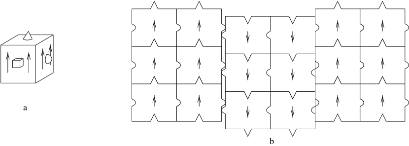
FIG. 2.: (a) Permanently magnetized particle lacking a $\theta$ operator. The arrows indicate the direction of magnetization. (b) Domain formation requires gaps between particles. A cross-section is shown.

REFERENCES

- [1] D. Ruelle, Helv. Phys. Acta 36, 183 (1963); D. Ruelle, Statistical Mechanics (W.A. Benjamin, Inc. 1969)
- [2] M.E. Fisher, Arch. Rat. Mech. Anal. 17, 377 (1964).
- [3] R.B. Griffiths, Phys. Rev. 176, 655 (1968).
- [4] W.F. Brown, Magnetostatic Principles in Ferromagnetism (North-Holland, Amsterdam, 1962).
- [5] N.D. Mermin Rev. Mod. Phys. 51, 591 (1979).
- [6] A. Ahroni, J.P. Jakubovics, IEEE Trans. Magn. 32 4463 (1996).
- [7] B. Groh and S. Dietrich, Phys. Rev. Lett. 79 749 (1997).
- [8] S. de Leeuw, J. Perram and E. Smith, Ann. Rev. Chem. 37, 245 (1986).
- [9] J.M. Deutch, Ann. Rev. Phys. Chem. 24, 301 (1973).
- [10] M.S. Wertheim, Ann. Rev. Phys. Chem. 30, 471 (1979).
- [11] Fisher [2] defined tempering with the stronger condition , but the weaker condition employed in equation (16) suffices.
- [12] C.P. Bean, J. Appl. Phys. 26, 1381 (1955).
- [13] H. Falk, Am. J. Phys 38, 858 (1970).
- [14] R.E. Rosensweig, Ferrohydrodynamics (Cambridge, 1985).
- [15] W. Luo, S.R. Nagel, T.F. Rosenbaum, and R.E. Rosensweig, Phys. Rev. Lett. 67, 2721 (1991).
- [16] D.D. Awschalom, et al., Phys. Rev. Lett. 68, 3092 (1992).
- [17] M. Abramowitz and I.A. Stegun, Handbook of mathematical functions with formulas, graphs and tables (Dover, 1965) Section 3.2; G.H. Hardy, J.E. Littlewood, and G. Polya, Inequalities (Cambridge University Press 1964), p. 26.
- [18] D. Wei and G.N. Patey, Phys. Rev. A 46, 7783 (1992).
- [19] M.J. Stevens and G.S. Grest, Phys. Rev. E 51, 5976 (1995)
- [20] D.W. Oxtoby, Chem. Phys. 69, 1184 (1978)
- [21] N.W. Ashcroft and N.D. Mermin, “Solid State Physics” (Rinehart and Winston, 1976).
- [22] G.N. Patey and J.P. Valleau, J. Chem. Phys. 64, 170 (1976)
- [23] M. Widom and H. Zhang, Phys. Rev. E 51 2099 (1995)
- [24] W.L. Jorgensen, J. Am. Chem. Soc. 103, 335 (1981)
- [25] D. Vanderbilt and R.D. King-Smith, Phys. Rev. B 48, 4442 (1993)
- [26] X. Gonze, Ph. Ghosez and R.W. Godby, Phys. Rev. Lett. 78, 294 (1997)
- [27] E.H. Lieb, Rev. Mod. Phys. 48, 553 (1976).
- [28] In this regard see B. Groh and S. Dietrich, Phys. Rev. Lett. 72, 2422 (1994), a comment by M. Widom and H. Zhang, Phys. Rev. Lett. 74, 2616 (1995), and a response by B. Groh and S. Dietrich, Phys. Rev. Lett. 74, 2617 (1995)
- [29] J.M Luttinger and L. Tisza, Phys. Rev. 70, 954 (1946).
- [30] P. Palfey-Muhoray, M.A. Lee, and R.G. Petscheck, Phys. Rev. Lett. 60, 2303 (1988).
- [31] D. Wei and G.N. Patey, Phys. Rev. Lett. 68, 2043 (1992); J.J. Weis, D. Levesque and G.J. Zarragoicoechea, Phys. Rev. Lett. 69, 913 (1992).
- [32] J. Reske et al., Phys. Rev. Lett. 75, 737 (1995); T. Albrecht et al., Appl. Phys. A 65 , 215 (1997)
- [33] P.G. de Gennes and P.A. Pincus, Solid State Commun. 7, 339 (1969).
- [34] J. C. Bacri and D. Salin, J. Physique. Lett. 43, L-649 (1982).
- [35] H. Wagner, in Hydrogen in metals I: Basic Properties, eds. G. Alefeld and J. Volkl (Springer, 1978) p. 5.
- [36] J. Tretkowski, J. Volkl, and G. Alefeld, Z. Physik B 28, 259 (1977).