Measurement of the hydrodynamic forces between two polymer-coated spheres

Abstract

The hydrodynamic forces between Brownian spheres are determined from a measurement of the correlated thermal fluctuations in particle position using a new method, two-particle cross-correlation spectroscopy (TCS). A pair of 1.3 $\mu$m diameter polymer-coated poly(methyl methacrylate) were held at separations of between 2$\mu$m and 20$\mu$m using optical traps. The mobility tensor is determined directly from the statistically-averaged Brownian fluctuations of the two spheres. The observed distance dependence of the mobility tensor is in quantitative agreement with low-Reynolds number calculations.

I Introduction

The hydrodynamic interactions between colloidal particles are important from both a fundamental and an industrial viewpoint. They determine, for instance, the rheological behaviour of suspensions, the kinetics of aggregation and phase separation and many other common colloidal phenomena Russel-648 . Yet despite this, the hydrodynamic properties of all but the simplest colloidal system have been a subject of considerable debate Segre-1121 . A key factor in this uncertainty has been the intrinsically long-ranged nature of the hydrodynamic coupling between solid particles. In the dilute limit, where it is sufficient to calculate just the leading order interaction, the solution of the stationary Stokes equation 1615 reveals that the interactions decay like the inverse separation (the Oseen tensor). The non-local nature of such interactions has led to considerable theoretical and numerical difficulties. Experiments have, conversely, also been problematic. Methods such as light scattering which have been used extensively in the past to probe the dynamics of concentration fluctuations provide only limited, indirect information on the microscopic nature of hydrodynamics in suspensions.

In this paper we report a detailed experimental study of the distance dependence of the hydrodynamic interactions between an individual pair of polymer-coated colloidal particles. Optical tweezers are used to hold two uncharged poly(methyl methacrylate) (PMMA) spheres apart at separations from between 2$\mu$m and 20$\mu$m. The hydrodynamic forces are measured using a new, highly sensitive, experimental technique, two-particle cross-correlation spectroscopy (TCS). TCS measures the statistically-averaged instantaneous fluctuations in position of two probe spheres. The in-plane position of each sphere is measured to nanometer precision using a quadrant photodetector. This technique is applied to a pair of colloidal particles suspended in a Newtonian liquid to yield a detailed direct test of low-Reynolds number predictions of hydrodynamic forces in a simple colloidal system.

Several reports of the test of theoretical predictions for the hydrodynamic coupling between a pair of spheres have already been published Crocker-882 ; Meiners-1501 . Our experiments differ in several regards. First, in the experiments reported to date, the surfaces of the colloidal spheres have been bare and not covered by a polymer layer. Since the adsorption or anchoring of a polymer onto the surface of a particle is a common method of imparting colloidal stability it is important to establish if the presence of a polymer layer modifies the hydrodynamic forces. Indeed theoretical calculations 1653 predict that, flow within the polymer layer, removes the divergence of the hydrodynamic forces seen at small pair-separations. Second, the reported experiments have used charged spheres at relatively low electrolyte concentrations (e.g. 0.1mM in Crocker-882 ) so that residual electrostatic interactions between the charged spheres or between the confined spheres and the walls complicates the interpretation. The experiments reported here used an uncharged colloid, for which previous work Pusey-853 ; Underwood-839 has shown that the interaction potential is well approximated by that of hard spheres.

Our paper is organised as follows: In the next section we describe the details of our experiment. Section III details the Brownian motion of an isolated sphere in a harmonic optical potential and describes the motion of a pair of dynamically-coupled spheres. We present our results in §IV before concluding.

II Experimental methods

Measurements were performed on a dilute suspension of uncharged poly(methyl methacrylate) (PMMA) spheres of radius 0.65 $\pm$ 0.02$\mu$m. To minimize the van der Waals forces between the PMMA spheres the surface of each sphere was covered with a covalently bound polymer brush ($\sim 100$Å thick) of poly(12-hydroxy stearic acid) Antl-63 . A dilute suspension of the spheres (volume fraction $\phi\sim 10^{-7}$) in a mixture of cyclohexane and cis-decalin was confined within a rectangular glass capillary, 170$\mu$m thick. The ends of the capillary were hermetically sealed with an epoxy resin to prevent evaporation and to minimize fluid flow. A small concentration of free polymer stabilizer was added to the suspension to reduce the adsorption of the spheres onto the glass surfaces of the cell.

A pair of spheres were trapped in a plane about 40$\mu$m above the lower glass surface of the cell using two optical traps. The traps were created by focusing orthogonally polarised beams from a Nd:YAG laser (7910-Y4-106, Spectra Physics) with a wavelength of $\lambda$ = 1064nm to diffraction-limited spots using an oil-immersion microscope objective (100x/1.3 NA Plan Neofluar, Zeiss). The resulting optical gradient forces localise the sphere near the focus of the beam. The centre-to-centre separation of the two traps could be varied continuously from between 2 and 30$\mu$m. Accurate positions for the optical traps were determined by digitising an image of two trapped spheres with a Imaging Technology MFG-3M-V frame grabber. The spheres’ locations were measured to within 40nm using a centroid tracking algorithm.

While the mean position of each sphere is fixed by the position of the corresponding laser beam, fluctuating thermal forces cause small but continuous displacements of the particle away from the centre of the trap. For small displacements the optical trapping potential is accurately described by a harmonic potential Tlusty-1543 . The restoring force on the particle is proportional to the displacement with a force constant which for a given particle and beam profile is a linear function of the laser power. In the experiments detailed below the intensities of the orthogonal beams were carefully adjusted until the stiffness of the two traps differed by less than 5%. The trap stiffness $k$ was typically of the order of 5.1 x 10^-6Nm^-1 which corresponds to a rms displacement within the trap of about 40nm. The intensity of each beam at the focal plane was estimated to be of the order of 30mW.

The positions of the two trapped spheres, ${\bm{r}}_{1}$ and ${\bm{r}}_{2}$, were tracked with nanometer resolution by observing the interference between the transmitted and scattered light in the back-focal plane of the microscope condenser using a pair of quadrant detectors 1614 . Difference voltages from the sum of the horizontal (X) and vertical (Y) halves of the quadrant detectors are linearly proportional to the displacement of the sphere from the optical axis of the trap. The trajectories, ${\bm{r}}_{1}(t)$ and ${\bm{r}}_{2}(t)$, were measured for a pair of spheres with mean separations $r=|{\bm{r}}_{1}-{\bm{r}}_{2}|$ from between 2.5$\mu$m and 20$\mu$m. For each value of $r$, the Brownian motion of the two spheres was followed for a total of 420s, at intervals of 50$\mu$sec, to yield 2²³ (8.4 x 10⁶) samples of the spheres’ dynamics.

III Brownian motion of confined spheres

III.1 An isolated sphere

A single hard sphere of radius $a$, moving with a constant velocity $\bm{{U}}$ through an unbounded fluid of viscosity $\eta$ experiences a hydrodynamic drag force $\bm{F_{D}}$ in the direction opposite to motion. In the low Reynolds number limit 1615 the velocity of the sphere is a linear function of the force exerted on the particle by the fluid,

$$\bm{U}=-b_{0}\bm{F_{D}}.$$ (1)

The constant $b_{0}$ is the mobility of an free particle which, if there is no slip at the boundary of the particle, is given by Stokes Law as

$$b_{0}=\frac{1}{6\pi\eta a}.$$ (2)

When the Brownian sphere is confined by a potential, $U(x)$, the drag force increases. The total force on the particle consists of a random Gaussian force $f(t)$ together with an additional force due to the potential field, $-dU/dx$. For a harmonic potential (of stiffness $k$) in the ‘long-time’ limit, where inertial terms are negligible, the motion of a confined Brownian sphere is described by the Langevin equation,

$$\frac{dx}{dt}=b_{0}[f(t)-kx(t)]$$ (3)

with a random particle force $f(t)$ which is Gaussian distributed with the moments,

$$\langle f(t)\rangle = 0$$

$$\langle f(t)f(t^{\prime})\rangle = 2b_{0}^{-1}k_{B}T\delta(t-t^{\prime}).$$ (4)

This Langevin equation is readily solved by standard methods Doi-646 and the position autocorrelation function $\langle x(t)x(0)\rangle$ determined. Since there is only one characteristic timescale in the long-time limit, the autocorrelation decays exponentially

$$\langle x(t)x(0)\rangle=\frac{k_{B}T}{k}\exp(-t/\tau)$$ (5)

with a decay time $\tau$ which is physically just the time taken by a sphere to diffuse a distance $l^{*}$,

$$l^{*}=\sqrt{\frac{2k_{B}T}{k}},$$ (6)

where $l^{*}$ is the classical turning point of the confining potential, or the separation at which the potential energy of the trapped sphere equals its thermal energy $k_{B}T$.

III.2 A pair of spheres

The motion of a pair of harmonically-bound particles differs from III.1 because the hydrodynamic forces couple the motion of the two spheres together. As one particle moves a flow is created in the surrounding fluid which drives fluctuations in the position of a neighbouring second sphere 1615 . In this section we analyze the correlated motion of a pair of particles which are coupled by such dynamic forces. We assume, for simplicity, that (1) the two trapped particles have the same diameters and are contained within optical traps with identical force constants; and (2) that there is no potential coupling between the two spheres.

The hydrodynamic forces acting between equal-sized spheres have been calculated by a number of authors Batchelor-618 ; 1666 ; Jeffrey-617 . In low-Reynolds number flow the hydrodynamic interactions between two spheres can be described by a set of linear relations between the force or torque exerted on a sphere and the corresponding translational and rotational velocities. If, as here, the spheres are freely rotating the applied torque must be zero and one can eliminate the angular velocities. In this case the linear relation between the forces and translational velocities defines the mobility tensor $\bm{b}_{ij}$,

$$\begin{pmatrix}\bm{U}_{1}\\ \bm{U}_{2}\end{pmatrix}=\begin{pmatrix}\bm{b}_{11}&\bm{b}_{12}\\ \bm{b}_{21}&\bm{b}_{22}\end{pmatrix}\begin{pmatrix}\bm{F}_{1}\\ \bm{F}_{2}\end{pmatrix}$$ (7)

where the two spheres are labeled $1$ and $2$ and the equivalence of the two particles implies that $\bm{b}_{11}=\bm{b}_{22}$ and $\bm{b}_{12}=\bm{b}_{21}$. The spherical symmetry of the Stokes limit reduces to one of axial symmetry and the mobility tensor depends crucially on the geometry of the two spheres Batchelor-618 . The linearity of the Stokes equation implies that each of the matrices $\bm{b}_{ij}$ can be decomposed into a pair of mobility coefficients which describes motion either along the line of the centres or perpendicular to it,

$$\bm{b}_{ij}(\bm{r})=A_{ij}(r)\frac{\bm{r}\bm{r}}{r^{2}}+B_{ij}(\bm{1}-\frac{\bm{r}\bm{r}}{r^{2}})$$ (8)

where the coefficients, $A_{ij}$ and $B_{ij}$, detail the longitudinal and transverse mobilities, respectively. In the remainder of this paper we shall confine our discussion to the longitudinal motion alone. In this case only two mobility coefficients are needed to quantify the hydrodynamic forces. Each of these mobilities, $A_{11}$ and $A_{12}$, is itself a function only of the normalised separation $\rho=r/a$ of the two spheres.

The mobility coefficient, $A_{12}$, couples the fluctuations along the line of the centres of the two spheres, chosen here as the $x$-axis, so that the particle coordinates, $x_{1}$ and $x_{2}$, are no longer independent. The extent of their correlation is determined from the solution of the Langevin equation

$$\begin{pmatrix}\dot{x}_{1}\\ \dot{x}_{2}\end{pmatrix}=\begin{pmatrix}A_{11}&A_{12}\\ A_{12}&A_{11}\end{pmatrix}\begin{pmatrix}f_{1}(t)-kx_{1}\\ f_{2}(t)-kx_{2}\end{pmatrix}$$ (9)

with the random force characterized by the moments

$$\langle f_{i}(t)\rangle = 0$$

$$\langle f_{i}(t)f_{j}(t^{\prime})\rangle = 2(A^{-1})_{ij}k_{B}T\delta(t-t^{\prime}).$$ (10)

and $(A^{-1})_{ij}$ as the inverse matrix of $A_{ij}$. Note that the mobility gradient terms, $k_{B}T/2\sum_{j}\partial A_{ij}/\partial x_{j}$, in the conventional Langevin equation have been ignored in equation 9 because in our experiments the positional fluctuations are typically two orders of magnitude smaller than the mean particle separation.

To solve this coupled Langevin equation we introduce the normal coordinates $X_{i}$,

$$X_{i}=\sum_{j}c_{ij}x_{j}$$ (11)

and choose the coefficients $c_{ij}$ so that the equation of motion for $X_{i}$ has the following form Wang-650 ,

$$\frac{dX_{i}}{dt}=-k\lambda_{i}X_{i}+F_{i}(t)$$ (12)

with $i$ = (1 or 2). It is readily shown that the matrix $c_{ij}$ consists of the normalised eigenvectors of the mobility matrix $A_{ij}$ so that the normal modes are

$$X_{1} = \frac{1}{\sqrt{2}}(x_{1}+x_{2})$$

$$X_{2} = \frac{1}{\sqrt{2}}(x_{1}-x_{2})$$ (13)

which describe, in turn, a symmetric collective motion ($X_{1}$) of the centre of mass of the two spheres and an antisymmetric relative motion ($X_{2}$) of the two spheres with respect to each other along the line of their centres. The mobilities $\lambda_{i}$ of the two modes are the eigenvalues of the matrix $c_{ij}$,

$$\lambda_{1} = A_{11}+A_{12}$$

$$\lambda_{2} = A_{11}-A_{12}.$$ (14)

while the $F_{i}$’s are random forces which satisfy

$$\langle F_{i}(t)\rangle = 0$$

$$\langle F_{i}(t)F_{j}(t^{\prime})\rangle = 2\delta_{ij}\lambda_{i}k_{B}T\delta(t-t^{\prime}).$$ (15)

Since the random forces are independent of each other, motion of the two normal modes are also independent of each other. The hydrodynamic term which couples the motion of the two spheres, $A_{12}$, leads to an asymmetry in the decay times of the normal modes. The time correlation functions of the normal coordinates are calculated readily from equation 12 as

$$\langle X_{i}(t)X_{j}(0)\rangle=\delta_{ij}\frac{k_{B}T}{k}\exp(-t/\tau_{i})$$ (16)

with decay times

$$\tau_{i}=\frac{1}{k\lambda_{i}}$$ (17)

Inverting the coordinate transformation of equation 11 gives the normalised time correlation functions of the particle centres

$$h_{ij}(t)=\frac{\langle x_{i}(t)x_{j}(0)\rangle}{\sqrt{\langle x_{i}^{2}\rangle\langle x_{j}^{2}\rangle}},$$ (18)

as

$$h_{11}(t) = \frac{1}{2}\bigl{[}\exp(-t/\tau_{1})+\exp(-t/\tau_{2})\bigr{]}$$

$$h_{12}(t) = \frac{1}{2}\bigl{[}\exp(-t/\tau_{1})-\exp(-t/\tau_{2})\bigr{]}.$$ (19)

Inspection reveals that the cross-correlation is very sensitive to the hydrodynamic coupling between the two spheres. At small times, $t\rightarrow 0$, $h_{12}$ records only the time-averaged, static correlations Chaikin-1263 which, at thermal equilibrium, depends only on the interparticle potential. In the current experiments there is no potential coupling between the two spheres and so $h_{12}(0)=0$. At long delay times, $t\rightarrow\infty$, the hydrodynamic flows which couples the motion decay to zero so that the positions of the two spheres are uncorrelated and $h_{12}(t\rightarrow\infty)=0$. The cross correlation is therefore zero both at short and long times. Equation III.2 reveals that the cross correlation will also be zero at intermediate times unless the two decay times, $\tau_{1}$ and $\tau_{2}$, differ. From equations 17 and III.2 this difference is a linear function of the hydrodynamic coupling term $A_{12}$. In the limit where $A_{12}\ll A_{11}$, which is the case in most physical situations, the cross-correlation has a minimum at a time which is fixed, to leading order, by the diagonal mobility $A_{11}$

$$t^{*}=\frac{1}{kA_{11}}\biggl{\{}1+\frac{1}{3}\biggl{(}\frac{A_{12}}{A_{11}}\biggr{)}^{2}+O\biggl{[}\biggl{(}\frac{A_{12}}{A_{11}}\biggr{)}^{4}\biggr{]}\biggr{\}}$$ (20)

while the depth of the minimum is determined by the ratio of the off-diagonal and diagonal mobilities

$$h_{12}(t^{*})=-\frac{1}{e}\biggl{\{}\frac{A_{12}}{A_{11}}+O\biggl{[}\biggl{(}\frac{A_{12}}{A_{11}}\biggr{)}^{3}\biggr{]}\biggl{\}}.$$ (21)

IV Results

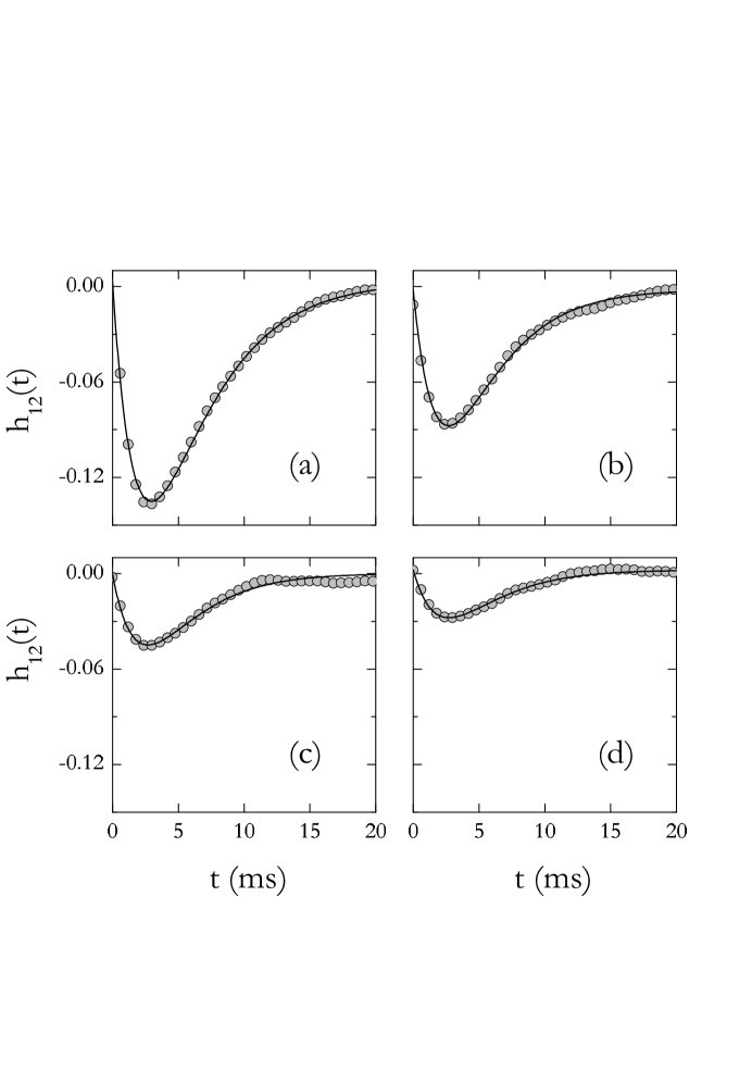
Figure 1: Cross correlation functions for 1.30 $\mu$m diameter PMMA spheres as a function of delay time $t$ and at four centre-to-centre separation $r$. (a) $r=2.47\mu$m, (b) $r=4.19\mu$m, (c) $r=7.44\mu$m, and (d) $r=11.47\mu$m. The motion is measured parallel to the separation vector. The solid line shows a fit to equation III.2. For clarity only every twelve data point is plotted.

The normalised longitudinal position cross correlation, $h_{12}(t)$, was measured for a pair of trapped spheres over a wide range of separations (2.5 $\mu$m $<r<20$ $\mu$m). Figure 1 shows typical data for four sphere separations. Three features in the experimental data are striking. First, the data show, rather surprisingly, that hydrodynamic interactions cause the two particles to be anti-correlated at intermediate times; second, the time at which the two particles are most strongly anti-correlated, the time $t^{*}$ at the minimum of $h_{12}$ , does not vary with the sphere separation; while conversely, the strength of the anti-correlation increases markedly as the separation $r$ reduces.

To interpret these observations the decay times $\tau_{1}$ and $\tau_{2}$ of the symmetric and anti-symmetric normal modes were extracted from a least squares fit of the data to equation III.2. The quality of the resulting fit may be gauged, for the four separation depicted in figure 1, by studying the solid curves, which are seen to accurately reproduce the measured data. From the experimentally determined decay times and trap stiffness the elements of the mobility tensor may be estimated as,

$$A_{11} = \frac{1}{2k}\biggl{(}\frac{1}{\tau_{1}}+\frac{1}{\tau_{2}}\biggr{)}$$

$$A_{12} = \frac{1}{2k}\biggl{(}\frac{1}{\tau_{1}}-\frac{1}{\tau_{2}}\biggr{)}.$$ (22)

The experimentally-determined scaled mobility elements, $b_{0}^{-1}A_{ij}(r)$, are plotted in figure 2 as a function of the dimensionless separation of the two spheres, $\rho=r/a$. The two mobilities show a strikingly different dependence on the sphere separation. While the diagonal mobility is largely unaffected by the sphere separation the off-diagonal term scales approximately inversely with $\rho$. These trends are, of course, consistent with the observations made above that the position, $t=t^{*}$, of the minimum in the correlation function does not shift with separation (see equation 20) while the depth increases with reducing separation (equation 21).

The experimental values for the mobilities may be compared with theoretical predictions for the hydrodynamic coupling of two hard spheres. Batchelor Batchelor-618 , for instance, has given the following expressions for the longitudinal mobilities,

$$b_{0}^{-1}A_{11} = 1-\frac{15}{4\rho^{4}}+O(\rho^{-6})$$

$$b_{0}^{-1}A_{12} = \frac{3}{2\rho}-\frac{1}{\rho^{3}}+O(\rho^{-7})$$ (23)

which are exact in the limit of large centre-to-centre separation $\rho$, as has been confirmed by 1666 . The solid curves in figure 2 show the predictions of the Batchelor Batchelor-618 theory for the longitudinal coupling. As is clear from this figure, the measured mobilities agree very well with the theoretical predictions over the entire experimentally accessible range of separations.

The deviations between theory and experiment evident in figure 2 are due largely to the experimental difficulty measuring the force constant $k$. This is seen in figure 3 where the experimentally determined mobility ratio, $A_{12}/A_{11}$, which from equation IV does not require any knowledge of $k$, is plotted as a function of the inverse separation $1/\rho$. The almost quantitative agreement seen, with no adjustable parameters, between the data and theory confirms the accuracy of Batchelor’s theoretical description of pair hydrodynamics. In addition the close agreement between experiment and theory suggests that, at least for the range of distances explored in the current experiments, the hydrodynamics forces between polymer-coated and uncoated spheres are very comparable.

V Discussion

We have presented a detailed experimental study of hydrodynamic coupling between an isolated pair of polymer-coated hard-sphere colloids. We find near quantitative agreement with Low Reynolds-number predictions for the hydrodynamic coupling between a pair of spheres. Surprisingly, we observe a strong anti-correlation in the positions of the two coupled spheres at intermediate times. At first sight this result looks counter-intuitive since one might expect naively a symmetric correlation between spheres. However the effect is a dynamic time-dependent phenomenon. The origin of which may be understood from the normal modes of the system. The motion of two spheres, along the line of their centres, decouples when analyzed in terms of a symmetric collective mode and an anti-symmetric relative mode. The mobilities of these independent modes are, from the asymptotic expressions of Batchelor Batchelor-618 and equation III.2,

$$\lambda_{1} = b_{0}\left\{1+\frac{3}{2\rho}-\frac{1}{\rho^{3}}-\frac{15}{4\rho^{4}}+O(\rho^{-6})\right\}$$

$$\lambda_{2} = b_{0}\left\{1-\frac{3}{2\rho}+\frac{1}{\rho^{3}}-\frac{15}{4\rho^{4}}+O(\rho^{-6})\right\},$$ (24)

where $\rho$ is the dimensionless centre-to-centre separation, $\rho=r/a$. Examination of the leading terms in this equation reveals that the mobility $\lambda_{1}$ of the symmetric mode is enhanced and the anti-symmetric mode reduced when compared with an isolated particle. The reduction in mobility of the anti-symmetric mode reflects the difficulty of squeezing fluid out of or into the narrow gap between two approaching spheres while the increased mobility for the symmetric mode is caused by the tendency for the fluid flow generated by one sphere to entrain a neighbouring sphere.

The asymmetry in the mobilities of the normal modes, seen in equation V, causes the decay times for thermal fluctuation in the two modes to differ. When the two spheres are close together, the mobility of the symmetric mode is enhanced compared with the anti-symmetric mode. As a consequence, symmetric fluctuations decay more rapidly than their anti-symmetric counterparts. At $t=0$ the proportions of thermally-excited symmetric and anti-symmetric fluctuations are equal since the positions of the two spheres are uncorrelated. With increasing time the amplitudes of both fluctuations decay. However the anti-symmetric fluctuations decay at a slower rate than the symmetric fluctuations so that the cross correlation develops a pronounced anti-correlation. The anti-correlation is however dynamical since over long time all fluctuations decay and the spheres become again uncorrelated.

In summary, we have shown that 2-particle cross-correlation spectroscopy (TCS) is a promising new technique for the quantitative determination of hydrodynamic interactions. TCS experiments are very flexible; the particle size, separation, potential interactions and indeed the dispersion medium can all be changed independently of each other. Variations of the methods described in this paper could, for instance, be used to follow the time course of collective fluctuations in a dense (host) complex fluid from the real-space trajectories of inserted probe colloidal particles. Currently, we are utilising TCS to study the many-body hydrodynamic interactions in concentrated particulate suspensions. Two probe PMMA particle are trapped within an index-matched silica suspension of volume fraction $\phi$. The resulting fluctuations in the trajectories of the two probe PMMA particles are used to determine the effective pair-mobility tensor in the suspension, as a function of particle separation and $\phi$. These measurements promise to provide new and detailed experimental information on the spatial and temporal development of hydrodynamic interactions in concentrated suspensions.

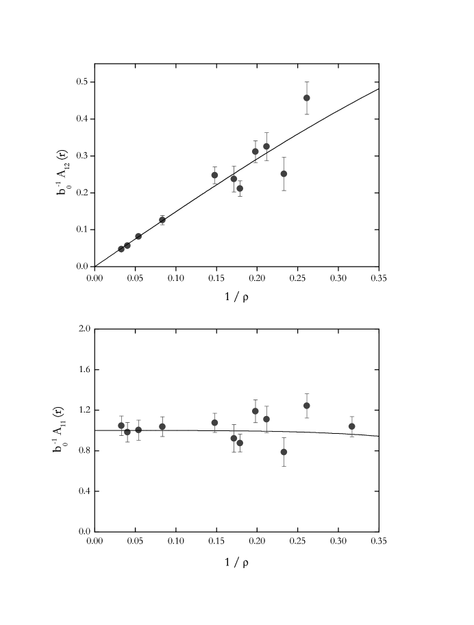
Figure 2: The experimentally-determined mobility coefficients, $b_{0}^{-1}A_{ij}$, for motion along the line of centres as a function of the inverse centre-to-centre separation $\rho=r/a$ . Here $b_{0}$ is the mobility of the PMMA particle of radius $a$. Solid lines show the predictions of low-Reynolds number hydrodynamic calculations for the case of two interacting solid spheres Batchelor-618 , with no adjustable parameters.

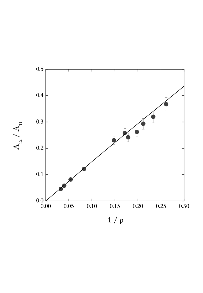
Figure 3: The experimental longitudinal mobility ratio $A_{12}/A_{11}$ as a function of the inverse sphere separation $\rho$, in units of the sphere radius. The solid line shows the predictions of Batchelor-618 .

- (1) W. B. Russel, D. A. Saville, and W. R. Schowalter, Colloidal Dispersions (Cambridge University Press, Cambridge, 1989).
- (2) P. N. Segre, E. Herbolzheimer, and P. M. Chaikin, Phys. Rev. Lett. 79(13), 2574 (1997).
- (3) J. Happel and H. Brenner, Low Reynolds Number Hydrodynamics (Prentice-Hall, London, 1965).
- (4) J. C. Crocker, J. Chem. Phys. 106, 2837 (1997).
- (5) J.-C. Meiners and S. R. Quake, Phys. Rev. Lett. 82, 2211 (1999).
- (6) A. A. Potanin and W. B. Russel, Phys. Rev. E 52(1), 730 (1995).
- (7) P. N. Pusey, in Liquids, Freezing and Glass transition, edited by J. P. Hansen, D. Levesque, and J. Zinn-Justin (North Holland, Amsterdam, 1991), NATO Advanced Study Institute at Les Houches, Session LI, 3-28 July 1989, pp. 763–942.
- (8) S. M. Underwood, J. R. Taylor, and W. van Megen, Langmuir 10, 3550 (1994).
- (9) L. Antl, J. W. Goodwin, R. D. Hill, R. H. Ottewill, S. M. Owens, S. Papworth, and J. A. Waters, Colloids Surf. 17, 67 (1986).
- (10) T. Tlusty, A. Meller, and R. Bar-Ziv, Phys. Rev. Lett. 81(8), 1738 (1998).
- (11) F. Gittes and C. F. Schmidt, Opt. Lett. 23(1), 7 (1998).
- (12) M. Doi and S. F. Edwards, The theory of polymer dynamics (Oxford University Press, New York, 1988).
- (13) G. K. Batchelor, J. Fluid. Mech. 74, 1 (1976).
- (14) B. Felderhof, Physica A 89A, 337 (1977).
- (15) D. J. Jeffrey and Y. Onishi, J. Fluid. Mech. 139, 261 (1984).
- (16) M. C. Wang and G. E. Uhlenbeck, Review of Modern Physics 17, 113 (1945).
- (17) P. M. Chaikin and T. C. Lubensky, Principles of Condensed Matter Physics (Cambridge University Press, Cambridge, 1995).