Correlated adaptation of agents in a simple market: a statistical physics perspective

Abstract

We discuss recent work in the study of a simple model for the collective behaviour of diverse speculative agents in an idealized stockmarket, considered from the perspective of the statistical physics of many-body systems. The only information about other agents available to any one is the total trade at time steps. Evidence is presented for correlated adaptation and phase transitions/crossovers in the global volatility of the system as a function of appropriate information scaling dimension. Stochastically controlled irrationally of individual agents is shown to be globally advantageous. We describe the derivation of the underlying effective stochastic differential equations which govern the dynamics, and make an interpretation of the results from the point of view of the statistical physics of disordered systems.

1 Introduction

There is currently much interest in the physics community in complex co-operative behaviour of systems of many individual entities influencing one another competitively. In particular, when combined with non-uniformity in the inclinations of the individuals, the behaviour of the whole can exhibit much greater complexity, richness and subtlety than is present in the rules governing individuals; in the words of P. W. Anderson “more is different” [1]. Examples are found in spin glasses (disordered magnetic alloys), neural networks and hard optimization problems (for recent reviews see [2, 3]). Economic markets also involve many individuals whose desires are not all simultaneously satisfiable and who often have different inclinations and strategies. It is therefore natural to ask to what extent the problems in physics and in economics are similar or different, to what extent the techniques and concepts developed for the physics problems can be applied to those in economics, to what extent the economics problems pose new challenges for the physicists and to search for fruitful symbiosis of understanding, quantification and application. To this end we discuss in this paper recent developments in the study of a model inspired by economics, but analyzed from the perspective of physics, finding unexpected new results and subtleties, and concluding that both subjects have something to teach each other and that there is potential for further transfers and discoveries. We make no attempt to be encyclopaedic or chronologically historical.

Before discussing the specific model, some general remarks are appropriate. Much of the progress in physics has come from starting with the simplest but non-trivial microscopic entities and interaction rules which can still lead to complex behaviour at the macroscopic level. Greater “reality” at the microscopic level can be added later. Many results are robust to the microscopic details, although new features can also arise with sufficient qualitative change. We apply a similar philosophy here, deliberately oversimplifying at the individual level to expose novel consequences of cooperation uncluttered by microscopic complication. Thus, we concentrate on systems with simple microscopic dynamical rules and minimal number of control parameters. In the spirit of statistical many-body theory we concentrate on systems with many ($N\gg 1$) microscopic players, with particular regard to the leading large-$N$ behaviour of macroscopic quantities. We allow for temporally-fixed variation among individuals but, in the spirit of statistical relevance, we draw their individual characteristics independently from identical distributions. We also allow for stochasticity (temporal indeterminacy) at the individual operational level, but again in a statistically relevant and minimal parameter fashion. As usual in statistical physics, we expect self-averaging of normal macroscopic observables, although non-self-averaging might be envisaged at a more sophisticated level [4, 3].

It is also appropriate to contrast our study with those of conventional economics theory. A typical assumption used in neoclassical economic theory [5] –especially game theory [6]– is that agents are hyper-rational. They know the utility functions of other agents, they are fully aware of the process they are embedded in, they make optimum long-run plans, and so forth. This is a rather extravagant and implausible model of human behaviour, especially in situations like a stock market. Moreover in neoclassical economic theory microscopic equilibrium is the reigning paradigm [5]. Individual strategies are assumed to be optimal given expectations, and expectations are assumed to be justified given the evidence. Equilibrium is thus reached in one-step dynamics once hyper-rationality is assumed. In this paper we consider a different, perhaps more realistic, scenario in which the only information available to any agent about the others is of the macroscopic consequences of the multiplicity of their actions (i.e. the analogues of market indices). We allow for diversity and irrationality in that they do not all draw the same conclusions from this information [7], nor do they necessarily operate deterministically. In general there will not be microscopic equilibrium although there may be macroscopic equilibrium.

The paper is organized as follows. In section 2 we present the Minority Game [8] and review its main features. This model is a specific realization of Arthur’s “El Farol” Bar Problem [7], and is the starting point of our investigations. In section 3 we consider a continuous generalization of the model, and study the effect of allowing for stochastic decision making on the part of the agents. The derivation of a fundamental analytic theory is discussed in section 4, where the underlying stochastic differential equations for the dynamics of the system are presented. Section 5 contains an interpretation of the results and we give our conclusions in section 6.

2 The Minority Game

The model system we consider is one known as Minority Game (MG) [8] and is intended to mimic in a simplified way a market of agents bidding to profit by buying when the majority wish to sell (so that the price can be lowered) and selling when the majority wish to buy (so that a higher price can be negotiated) [7]. It comprises a large number of agents each of whom can act as buyer or seller, deciding on how to play at each time-step through the application of a personal strategy to commonly available information. Each agent has a small set of available strategies, drawn randomly, independently and immutably with identical probabilities from a large suite of strategies. At each time step each agent picks one of his or her strategies, based on points allocated cumulatively to the strategies according to their (virtual) performance in predicting the minority action. For simplicity no other rewards are given.

The system has quenched (fixed in time) randomness in the set of strategies picked at the start of the game by each agent, and it has frustration in that the rewards are for minority action, so not all the individual inclinations can be satisfied simultaneously. There is no direct interaction between agents. Nevertheless, correlation does arise through the adaptive evolution of the use of strategies and manifests itself in the interesting non-trivial macroscopic behaviour of the system.

In the original formulation of the MG [8] agents could only make two choices, buy or sell, with no weight attributed to the size of the order. Conventionally, the strategy points are set initially to zero and thus the agents start making their first choice at random. The common information on which they based their decisions was the minority choice (buy or sell) over the last $m$ time-steps. The strategies were quenched randomly-chosen Boolean functions acting on this information, the binary output determining the buy/sell decision. The strategy used by any agent at any time was the one with the currently greatest point-score from those at his/her disposal. Numerical simulations showed [9] that while the average in time (and over the realizations of the disorder) of the total action was just an equality of buyers and sellers, due to the symmetric nature of the model, the standard deviation of its fluctuations away from this value (the analogue of the volatility of a conventional stockmarket) displayed remarkable structure. As a function of the “memory” $m$, the volatility has two regimes: for low values of $m$, the volatility is larger than the value corresponding to all agents just playing randomly; it decreases monotonically with increasing $m$, crosses the value corresponding to random behaviour, and reaches a minimum at a critical value of the memory $m_{c}$; it then starts to grow monotonically with $m$, asymptotically approaching the random value from below. This non-trivial behaviour of the fluctuations was interpreted as an indication of a cooperative “phase transition” in the system [9, 10] (see, eg., [11], for a introduction to phase transitions). Simulations also showed [9] that the relevant scaling variable was the reduced dimension of the space of strategies $d=2^{m}/N$, and that the volatility scaled with the number of agents as $\sqrt{N}$.

A second interesting observation was made in [12], where it was shown numerically that that the macroscopic behaviour of the MG was unaffected by replacing the time history by an artificial history, chosen randomly and independently at each time-step from the space of all possible histories with uniform probability, provided all agents received the same bogus information (and that the point-scores were still updated on the basis of performance). This is a consequence of the ergodic nature of the MG [13], and indicates that the principal role of the information is in providing a correlation mechanism between the agents in terms of the strategies used. This observation offers a great simplification for the analysis of the model, since replacing the true history by just external noise allows us to study a simpler system which is stochastic but local in time, instead of the more difficult original problem which is deterministic but non-local in time (see also [14]). In fact, we shall also see the consequence of allowing for a further different kind of stochasticity in the next section.

3 The Thermal Minority Game

As discussed in the introduction, it is natural to expect that the qualitative features of the MG are robust under changes in the microscopic detail of the model. In this section we present a generalization of the MG to continuous degrees of freedom and to allow for stochastic decision making on part of the agents, known as the Thermal Minority Game (TMG), and first introduced in [13]. This generalization not only preserves the main features of the MG discussed so far, but also gives interesting and advantageous new behaviour, and enables a simpler analytic description of the coarse-grained microdynamics of the system.

3.1 Continuous MG

The continuous version of the MG is as follows [13]. The system consists again of $N$ agents playing the game. At each time step $t$, each agent reacts to a common piece of “information” $\vec{\cal I}(t)$, by taking an action or bid $b_{i}(t)$ ($i=1,\dots,N$). Following the observation of [12] the information $\vec{\cal I}(t)$ is taken to be a random noise, defined as a unit-length vector in a $D$-dimensional space, for instance ${\mathbb{R}}^{D}$, $\delta$-correlated in time and uniformly distributed on the unit sphere. The bid $b(t)$ is defined to be a real number, which can be interpreted as placing an order in a market, of size $|b(t)|$ and positive/negative meaning buy/sell. Bids are prescribed by strategies: maps from information to bid, ${\mathbb{R}}^{D}\to{\mathbb{R}}$. For simplicity the strategy space $\Gamma$ of the model is restricted to the subspace of homogeneous linear mappings, in contrast to the whole space of binary functions in the MG. Thus a strategy $\vec{R}$ is defined as a vector in ${\mathbb{R}}^{D}$, subject for normalization to the constraint $\|\vec{R}\|=\sqrt{D}$, and the prescribed bid is the scalar product $\vec{R}\cdot\vec{\cal I}(t)$. Each agent has $S$ strategies, drawn randomly and independently from $\Gamma$ with uniform distribution, remaining fixed throughout the game. In what follows we will focus for simplicity on the case of two strategies per agent, $S=2$, the generalization to $S>2$ being straightforward (and the case $S=1$ being trivial, since there is no possibility of adaptation on the part of the agents). At time step $t$ each agent $i$ chooses one of his/her strategies $\vec{R}^{\star}_{i}(t)$ to play with. The “total bid” (or “excess demand”) is then $A(t)\equiv\sum_{j}b_{j}(t)=\sum_{j}\vec{R}^{\star}_{j}(t)\cdot\vec{\cal I}(t)$. The agents keep track of the potential success of the strategies by assigning points to them, which are updated according to $P(\vec{R},t+1)=P(\vec{R},t)-A(t)\,b(\vec{R})/N$, where $P(\vec{R},t)$ represents the points of strategy $\vec{R}$ at time $t$.

Let us now see whether the results obtained with this continuous formulation of the MG are the same as in the original binary setup. To this end we first review the results of simulations. The average of the total bid $A(t)$ over time and quenched disorder is zero, as is expected from the symmetric nature of the model. As discussed in the previous section, the first relevant macroscopic observable is the standard deviation $\sigma$ of the total bid, or volatility, $\sigma^{2}\equiv N^{-1}\overline{\langle A^{2}(t)\rangle}$, where the overline means disorder average, $\langle\cdot\rangle\equiv\lim_{t\to\infty}\frac{1}{t}\int_{t_{0}}^{t_{0}+t}(\cdot)\,dt^{\prime}$, and we have normalized $\sigma$ by $\sqrt{N}$ according to the findings of [9]. In Fig. 1 we show that the main features of the MG are reproduced: first, the relevant scaling parameter is the reduced dimension of the strategy space $d=D/N$; second, the volatility starts for low $d$ at a value larger than the one corresponding to the agents choosing randomly, $\sigma_{r}=1$ in this case, decreases monotonically until it reaches a minimum at $d=d_{c}(S)$, the minimum being shallower the higher is the number of strategies $S$ [15], and then it approaches $\sigma_{r}$ asymptotically from below. It is easy to check that all the other standard features of the binary model are reproduced in the continuous formulation.

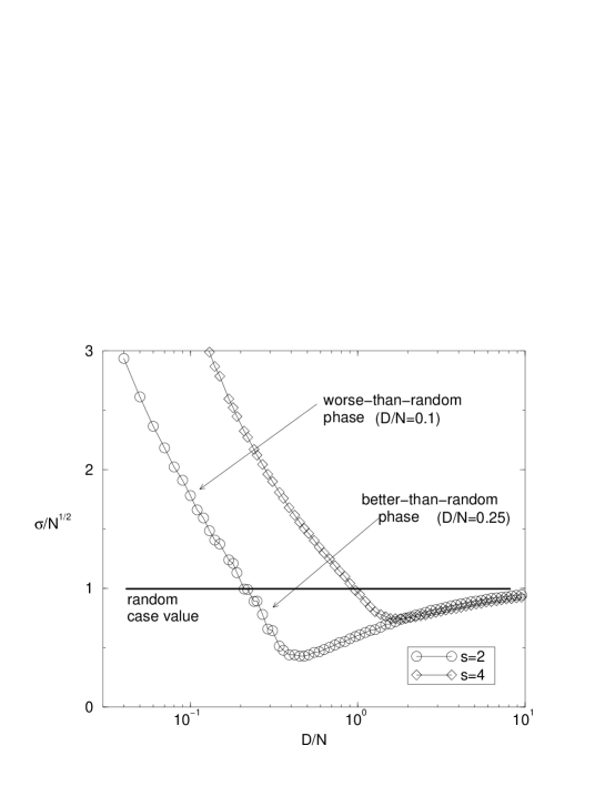
Figure 1: Continuous formulation of the MG [13]: The scaled volatility $\sigma/\sqrt{N}$ as a function of the reduced dimension $D/N$, at $S=2$ and $S=4$. The horizontal line is the variance in the random case. The total time $t$ and the initial time $t_{0}$ are $10000$ steps. Average over $100$ samples, $N=100$.

3.2 Stochastic decision making

In the original formulation of the MG the agents played in a deterministic fashion using their ‘best’ strategies, the ones with the highest number of points. In this subsection we introduce indeterminacy (irrationality) on the part of the agents and show this it can be advantageous.

In the TMG a natural generalization to non-deterministic behaviour is allowed [13]. At time step $t$, each agent $i$ chooses $\vec{R}^{\star}_{i}(t)$ randomly from his/her $\{\vec{R}_{i}^{a}\}$ with probabilities $\{\pi_{i}^{a}(t)\}$ ($a=1,\ldots,S$). The probabilities $\pi^{a}_{i}(t)$ are functions of the points parameterized by a “temperature” $T$, defined so as to interpolate between the MG case at $T=0$, all the way up to the totally random case $\pi_{i}^{a}=1/S$ at $T=\infty$. The temperature can be thought of as a measure of the power of resolution of the agents: when $T=0$ they are perfectly able to distinguish which are their best strategies, while for increasing $T$ they are more and more confused, until for $T=\infty$ they choose their strategy completely at random. In the language of Game Theory, when $T=0$ agents play ‘pure’ strategies, while at $T>0$ they play ‘mixed’ ones [6].

We now consider the consequences of having introduced the temperature. For simplicity we assume $S=2$. For the probabilities we choose the form $\pi^{1,2}_{i}(t)\propto\exp{[\pm\beta\;\mbox{sgn}(p_{i}(t))]}$ (with $\sum_{a}\pi^{a}_{i}(t)=1$ and $\beta=1/T$) [19], which satisfies the requirements of the previous paragraph. Consider now a value of $d$ belonging to the worse-than-random region of the MG (see Fig.1) and let us see what happens to the volatility $\sigma$ when we switch on the temperature. We know that for $T=0$ we must recover the same value as in the ordinary MG, while for $T\to\infty$ we expect to obtain the value $\sigma_{r}$ of random choice. But in between a very interesting thing occurs: $\sigma(T)$ is not a monotonically decreasing function of $T$, but there is a large intermediate temperature regime where $\sigma$ is smaller than the random value $\sigma_{r}$; see Fig.2. The meaning of this result is the following: even if the system is in a MG phase which is worse than random, there is a way to significantly decrease the volatility $\sigma$ below the random value $\sigma_{r}$ by not always using the best strategy, but rather allowing a certain degree of individual error.

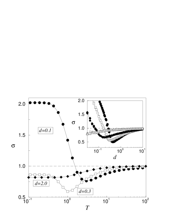
Figure 2: TMG: Volatility as a function of the temperature for the case of probabilities $\pi^{1,2}_{i}(t)\propto\exp{[\pm\beta\;\mbox{sgn}(p_{i}(t))]}$. Inset: volatility as a function of $d$ for different values of the temperature $T=10^{-3},\,1,\,2,\,10$.

Furthermore, even if we fix $d$ at a value belonging to the better-than-random region, but with $d<d_{c}$, a similar range of temperature still improves the behaviour of the system, decreasing the volatility even below the MG value (see Fig. 2). In the phase $d>d_{c}$ the behaviour changes; the optimal value of $\sigma$ is at $T=0$, and the volatility simply increases with increasing temperature towards $\sigma_{r}$, as shown in Fig. 2.

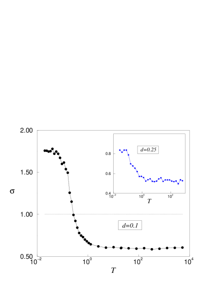
Figure 3: (a) TMG: Volatility as a function of the temperature $T$ at $d=0.1$, for the case $\pi^{a}_{i}(t)\propto\exp{[\beta P(\vec{R}_{i}^{a},t)]}$, for finite waiting time. In the inset we show $d=0.25$.(b) The same as in (a) for waiting times larger than $NT$.

Another possible functional form for the probabilities is $\pi^{a}_{i}(t)\propto\exp{[\beta P(\vec{R}_{i}^{a},t)]}$. For long but finite simulation time this yields the results shown in Fig. 3a [13], which are analogous to those of Fig. 2. However, the upturn of $\sigma$ for large temperatures for this choice of probabilities is only a transient [16, 17, 18]: for any $T\gg 1$, if one waits for times of order $NT$ the volatility stays at its smallest possible value; see Fig. 3b. Thus, we see that in the $d<d_{c}$ phase, for any finite temperature the performance of the system will be better than the original MG, and for any finite temperature $T>{\cal O}(1)$ the performance will be optimal, provided one waits long enough.

4 Continuous time dynamics of the TMG

In this section we derive the continuous time limit of the TMG as a starting point for the analytical study of its dynamics [19]. We do this in two steps. We first show that, to a good approximation, the external information can be eliminated in favour of an effective interaction between the agents. We then cast the dynamical equations of the TMG as a set of stochastic differential equations for an interacting disordered system with nontrivial random diffusion. Again, for simplicity, we consider explicitly $S=2$.

The set of unconstrained degrees of freedom of the TMG is given by the differences $\{p_{i}(t)\}$ of the points of the two strategies of each agent. The choice of strategies used at each stage is given by $\vec{R}^{\star}_{i}(t)=\vec{\omega}_{i}+\vec{\xi}_{i}\,\mbox{sgn}\left[s_{i}(t)+\mu(t)\right]$, where $\vec{\omega}_{i}\equiv\left({\vec{R}}_{i}^{1}+{\vec{R}}_{i}^{2}\right)/2$, $\vec{\xi}_{i}\equiv\left({\vec{R}}_{i}^{1}-{\vec{R}}_{i}^{2}\right)/2$, $s_{i}(t)\equiv\pi_{i}^{1}(t)-\pi_{i}^{2}(t)$, and $\mu(t)$ is a stochastic random variable uniformly distributed between $-1$ and $1$ and independently distributed in time. The equations for the point differences then read,

$$p_{i}(t+1)=p_{i}(t)-{\vec{a}}(t)\cdot{\vec{\cal I}}(t)\,\vec{\xi}_{i}\cdot{\vec{\cal I}}(t),$$ (1)

where ${\vec{a}}(t)\equiv\sum_{i}\vec{R}^{\star}_{i}(t)/N$. Eqs. (1), together with the random processes for ${\vec{\cal I}}(t)$ and ${\vec{R}}_{i}^{\star}(t)$, define the dynamics of the TMG.

We now consider the continuous time limit of Eqs. (1) in such a way as to preserve all the macroscopic features of the TMG. To this end we introduce an arbitrary time step $\Delta t$. We deal first with the information ${\vec{\cal I}}(t)$. Let us assume that ${\vec{\cal I}}(t)$ is a differential random motion in the space of strategies, i.e., ${\vec{\cal I}}(t)=\Delta\vec{W}(t)$, with zero mean and variance $\Delta t$. Replacing in Eqs. (1) we obtain $p_{i}(t+\Delta t)=p_{i}(t)-{\vec{a}}(t)\cdot\Delta\vec{W}(t)\,{\vec{\xi}}_{i}\cdot\Delta\vec{W}(t)$. In the limit $\Delta t\to 0$, and using the Kramers-Moyal expansion [20], we get

$$dp_{i}(t)=-\frac{1}{ND}\sum_{j}\vec{R}^{\star}_{j}(t)\cdot{\vec{\xi}}_{i}\,dt+{\cal O}(dt^{2}).$$ (2)

Note that to ${\cal O}(dt)$ the noise has been eliminated in favour of an effective strategy interaction among the agents, and the standard deviation becomes

$$\sigma^{2}=\frac{1}{ND}\overline{\bigg{\langle}\sum_{ij}\vec{R}^{\star}_{i}(t)\cdot\vec{R}^{\star}_{j}(t)\bigg{\rangle}}.$$ (3)

When the temperature is different from zero the TMG Eqs. (2) still depend on the stochastic choice of strategies ${\vec{R}}_{i}^{\star}(t)$, even at leading order. At each time step, ${\vec{R}}_{i}^{*}$ takes one of the two possible values ${\vec{R}}_{i}^{1,2}$, defining a stochastic jump process. In order to write the corresponding Master Equation we need to know the transition probabilities. The r.h.s. of Eq. (2), which we denote $\Delta_{i}$, is a normalized sum of $N$ random numbers ${\vec{\xi}}_{i}\cdot{\vec{R}}_{j}^{\star}(t)$, each with mean $m_{ij}={\vec{\xi}}_{i}\cdot{\vec{\omega}}_{j}+{\vec{\xi}}_{i}\cdot{\vec{\xi}}_{j}\,s_{j}(t)$, and variance $v_{ij}=({\vec{\xi}}_{i}\cdot{\vec{\xi}}_{j})^{2}[1-s_{j}^{2}(t)]$. By the central limit theorem, we know that for $N$ large $\Delta_{i}$ will tend to be normally distributed with mean $\langle\langle\Delta_{i}\rangle\rangle=\sum_{j}m_{ij}$, and variance $\langle\langle\Delta_{i}^{2}\rangle\rangle=\sum_{j}v_{ij}$, where $\langle\langle\cdot\rangle\rangle$ stands for average over realizations of the random process $\mu(t)$. Moreover, $\Delta_{i}$ and $\Delta_{j\neq i}$ are correlated, the covariance matrix given by

$$M_{ij}[{\mathbf{p}}(t)]\equiv\langle\langle\Delta_{i}\,\Delta_{j}\rangle\rangle-\langle\langle\Delta_{i}\rangle\rangle\langle\langle\Delta_{j}\rangle\rangle=\sum_{k}{\vec{\xi}}_{i}\cdot{\vec{\xi}}_{k}\,{\vec{\xi}}_{j}\cdot{\vec{\xi}}_{k}\left[1-s_{k}^{2}(t)\right],$$ (4)

where ${\mathbf{p}}\equiv(p_{1},\ldots,p_{N})$, etc. Collecting these results, we obtain the transition probabilities in the large $N$ limit, $W({\mathbf{p}}^{\prime}|{\mathbf{p}})=\Phi(\nabla_{\mathbf{s}}{\cal H};{\mathbb{M}})$, where $\Phi$ corresponds to the normal distribution with mean $\nabla_{\mathbf{s}}{\cal H}$ and covariance matrix ${\mathbb{M}}\equiv\{M_{ij}\}$, where the “Hamiltonian” $\cal H$ is given by

$${\cal H}=\frac{1}{2}\Omega+\sum_{i}h_{i}s_{i}+\frac{1}{2}\sum_{ij}J_{ij}s_{i}s_{j},$$ (5)

with

$$h_{i}\equiv\sum_{j}{\vec{\omega}}_{j}\cdot{\vec{\xi}}_{i}/ND,\;\;\;J_{ij}\equiv{\vec{\xi}}_{j}\cdot{\vec{\xi}}_{i}/ND.$$ (6)

Note that $\partial{\cal H}/\partial s_{i}\sim{\cal O}(1)$, and $M_{ij}\sim{\cal O}(1/N)$, so that fluctuations are also of ${\cal O}(1)$ and thus are not suppressed when $N\to\infty$.

The $\mu(t)$ are chosen independently at each time. If we make the natural assumption that in the limit $dt\to 0$ their correlation at different times is a $\delta$-function, the Master Equation becomes a Fokker-Planck equation by means of Kramers-Moyal expansion [20]

$$\frac{\partial{\cal P}}{\partial t}=-\sum_{i}\frac{\partial}{\partial p_{i}}\left(\frac{\partial{\cal H}}{\partial s_{i}}\,{\cal P}\right)+\frac{1}{2}\sum_{ij}\frac{\partial^{2}}{\partial p_{i}\partial p_{j}}\left(M_{ij}\,{\cal P}\right).$$ (7)

The dynamics of the TMG is therefore effectively described by a set of stochastic differential equations for the point differences

$$d{\mathbf{p}}=-\nabla_{\mathbf{s}}{\cal H}\,dt+{\mathbb{M}}\cdot d{\mathbf{W}},$$ (8)

where ${\mathbf{W}}(t)$ is an $N$-dimensional Wiener process, and the volatility is given by $\sigma^{2}=2\overline{\langle{\cal H}\rangle}+\sum_{i}\overline{J_{ii}}-\sum_{i}\overline{J_{ii}\langle s_{i}^{2}\rangle}$.

A detailed interpretatin of ${\cal H}$ is given in the next section, but briefly eq. (8) is suggestive of it as controlling energy with the ‘motion’ of ${\mathbf{p}}$ given by its derivative. However we note that for a natural analogue of Newton’s law or its generalization to a noisy environment, as in the Langevin equation, the derivative would be with respect to ${\mathbf{p}}$, whereas here it is with respect to ${\mathbf{s}}$ (which is a function of ${\mathbf{p}}$), so that a metric is needed to relate $d{\mathbf{p}}/dt$ to the natural force $\nabla_{\mathbf{s}}{\cal H}$. At finite temperature one also has the unusual extra diffusive/noise term ${\mathbb{M}}\cdot d{\mathbf{W}}$. An investigation based on replacing $\nabla_{\mathbf{s}}{\cal H}$ by $\nabla_{{\mathbf{p}}}{\cal H}$ and ingnoring the diffusive term was performed in [26].

5 Interpretations

Notwithstanding the subtleties mentioned in the last paragraphs, it is interesting to consider the implications of ${\cal{H}}$ as a controlling function of the dynamics. The form of ${\cal{H}}$ exhibited in Eq. (5) is a familiar one in statistical physics, with $-J_{ij}$ interpreted as measuring the strength of correlation between spins $s_{i}$ and $s_{j}$ and $-h_{i}$ as a (magnetic) field acting on $s_{i}$ and trying to “orient” it. Hence is formally justified the interpretation of common ‘information’, to which all respond, as providing a mechanism of effective mutual interaction. More particularly, taking account of the random character of $\{h_{i}\}$ and $\{J_{ij}\}$, ${\cal{H}}$ is reminiscent of the Sherrington-Kirkpatrick model [24] of a spin glass and the Hopfield model [25] of a neural network, in both cases augmented by random fields [2]. In the SK model the $J_{ij}$ are chosen randomly from a distribution with variance scaling as $N^{-1}$, while for the Hopfield model $J_{ij}$ is as given in Eq. (6), but with opposite sign and where the Cartesian components of $\{{\vec{\xi}}_{i}\}$ correspond to memorized patterns of activity. In both of these models (SK and Hopfield) the ground state energy (minimum of the corresponding ${\cal{H}}$) is less than the energy associated with a paramagnet (value of ${\cal{H}}$ corresponding to random $\{s_{i}\}$) due to judicious correlation of the $\{J_{ij}\}$ and $\{s_{i}\}$, even with all the $\{h_{i}\}=0$. It is then natural to ask whether a similar correlation is responsible for the reduction of the volatility of the MG below that for random operation. This is however not the case: in Fig. 4 [32] we show the result of numerical simulations of a system in which the second strategy of each agent ${\vec{R}}^{2}_{i}$ is exactly the opposite of its first strategy, that is ${\vec{R}}^{2}_{i}=-{\vec{R}}^{1}_{i}$ (with ${\vec{R}}^{1}_{i}$ still chosen randomly at the start of the game), so that all the $h_{i}$ are zero, and we note that $\sigma$ never falls below the random value. Clearly, the random field term is crucial in reducing the volatility advantageously [10, 31].

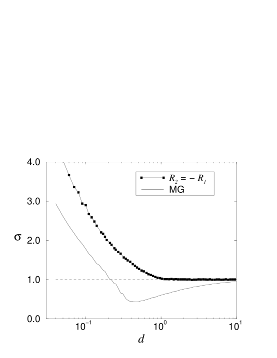
Figure 4: Volatility for anticorrelated strategies $\vec{R}^{2}_{i}=-\vec{R}_{i}^{1}$ (squares) compared with the standard MG (solid line).

The first term in the dynamical equations (8) corresponds (up to a factor) to gradient descent in the surface defined by ${\cal H}$. The natural question then is whether the asymptotic states reached by the dynamics are given by the typical extrema of ${\cal H}$, which would imply that in the long run the system reaches macroscopic equilibrium. This issue was explored in [26] (see also [27]), where ${\cal H}$ was minimized employing techniques developed for the statistical mechanics of spin glasses [28, 24] and adapted for neural networks [29] (for reviews see [4, 30, 3]). An excellent agreement with the numerics of the MG was found in the phase $d>d_{c}$, but this method failed to reproduce the behaviour in the $d<d_{c}$ phase (see Fig.5), although an equilibrium transition was found at a value of $d$ close to $d_{c}$.

This seems to suggest that the behaviour of the MG in the $d<d_{c}$ phase is dynamical in nature. A simple test is the sensibility to initial conditions. In Fig. 5 we show the results of simulating the original dynamics Eqs. (1) of the MG starting from any initial conditions with $|p_{i}(0)|\sim{\cal O}(1)$ [19], instead of the conventional choice of $p_{i}(0)=0$. We can see that the the behaviour of the system is very different in the region $d<d_{c}$: after an initial transient, the variance falls below the initial random value and stays in the better-than-random phase for all values of $d$. This sensitivity of the results to the initial conditions is a clear indication that the system does not equilibrate for $d<d_{c}$. An important open problem in the MG is finding the relation between the equilibrium (static) phase transition obtained from minimization of the Hamiltonian ${\cal H}$ [26] and the actual dynamical transition observed in the simulations.

Figure 5: Volatility as a function of $d$ for random initial conditions (squares) compared with the standard MG (solid line). Dotted line corresponds to the approximation of [26].

The differential equations (7) and (8) provide the basis for development of a macroscopic dynamics, either via the dynamical replica theory of Coolen and Sherrington [33] or via the generating functional approach [34]. However, we defer this discussion to later papers.

Finally we remark on the relationship with the crowd-anticrowd concept of [35], where a crowd is a group of agents playing the same strategy and the corresponding anticrowd play the opposite one. The proposal of [35] is that the macroscopic properties of the MG can be described by the behaviour of the crowd-anticrowd pairs. In this approach the volatility of the system is approximated as the sum over all the pairs of crowd-anticrowds of the square of the difference of their sizes. We can formalize this concept in the continuous formulation of the MG by defining the crowd-anticrowd pairs in terms of the projection of the strategies used by the agents on an arbitrary orthonormal basis $\{{\hat{e}}_{\mu}\}\;(\mu=1,\ldots,D)$ of the strategy space: $N_{\mu}-N_{\bar{\mu}}\equiv\sum_{i}{\hat{e}}_{\mu}\cdot{\vec{R}}^{\star}_{i}$. This definition is analogous to that of “staggered” magnetizations in a spin system or a neural network [29]. If we write the volatility using the approximation of [35] $\sigma^{2}=\frac{1}{N}\sum_{\mu}(N_{\mu}-N_{\bar{\mu}})^{2}$, and make use of the completeness relation of the $\{{\hat{e}}_{\mu}\}$, we recover Eq. (3). Moreover, an effective dynamics of crowds-anticrowds, as proposed in [36], is exactly derivable from the microscopic dynamical equations (8).

It is of course interesting to aks about the stability of our conclusions to minor perturbations of the model. We have already noted the stability of the qualitative features of the original minority game to a change in the number of strategies per agent (excluding the special case $S=1$). This continues to the thermal extension. We have not investigated explicitly changes to the learning rule but it seems reasonable to expect qualitatively analogous behaviour for other generalized minority rules, for example non-linear rewards but still favouring minority action [37]. Reward rules involving capital accumulation and consequent variation of potential market influence [38] are another natural extension, as also evolution of the strategies themselves [39, 40]

6 Conclusion

In this paper we have discussed the application of techniques and philosophy of the statistical physics of complex cooperative frustrated many-body systems to a simple model of agents in a competitive market. We have shown that this can lead to both qualitatively and quantitatively new results in the economics-inspired model and also, conversely, that economics models can yield new challenges for statistical physics. The techniques have included computer simulation and analysis. In the simulations we have concentrated on the macroscopic steady-state. In the analysis we have derived a potentially useful microscopic formulation in terms of stochastic differential equations, itself different and more subtle that that normally encountered in conventional condensed-matter statistical physics at the corresponding coarse-grained microscopic level. The challenge still remains to develop a full macrodynamics, both equilibrium and out-of-equilibrium, but the derived microdynamics is the necessary ingredient for extension of relevant techniques from statistical physics.

We have restricted discussion to a model which is clearly oversimplified from the perspective of a true economic market, but it is possible to envisage still simplified but more realistic models which should be capable of more truly analysing the meaning of “efficiency” and going beyond it.

References

References

- [1] P.W. Anderson 1972 More is different - broken symmetry and nature of hierarchical structure in science, Science 177, 393.
- [2] A.P. Young (editor) 1998 Spin glasses and random fields (World Scientific, Singapore).
- [3] D. Sherrington 1999 Spin glasses in Physics of novel materials edited by M.P. Das (World Scientific, Singapore), 146.
- [4] M. Mézard, G. Parisi and M.A. Virasoro 1987 Spin glass theory and beyond (World Scientific, Singapore).
- [5] See, e.g., D.M. Kreps 1990 A Course in Microeconomics Theory (Harvester Wheatsheaf, New York).
- [6] D. Fudenberg and J. Tirole 1991 Game Theory (MIT Press, Cambridge, Massachussets).
- [7] W.B. Arthur 1994 Inductive Reasoning and Bounded Rationality, Am. Econ. Rev. 84 406.
- [8] D. Challet and Y-C. Zhang 1997 Emergence of Cooperation and Organization in an Evolutionary Game, Physica A 246, 407.
- [9] R. Savit, R. Manuca and R. Riolo 1999 Adaptive competition, market efficiency, and phase transitions Phys. Rev. Lett. 82, 2203.
- [10] D. Challet and M. Marsili 1999 Phase transition and symmetry breaking in the minority game, Phys. Rev. E 60, R6271.
- [11] J.M. Yeomans 1992 Statistical Mechanics of Phase Transitions (Oxford University Press, Oxford).
- [12] A. Cavagna 1999 Irrelevance of memory in the minority game, Phys. Rev. E 59, R3783.
- [13] A. Cavagna, J.P. Garrahan, I. Giardina and D. Sherrington 1999 Thermal model for adaptive competition in a market, Phys. Rev. Lett. 83, 4429.
- [14] D. Challet and M. Marsili 2000 Relevance of memory in minority games, Phys. Rev E 62, 1862.
- [15] D. Challet and Y.-C. Zhang 1998 On the minority game: Analytical and numerical studies, Physica A 256, 514.
- [16] G. Bottazzi, G. Devetag and G. Dosi 1999 Learning and Emergent Coordination in Speculative Markets: Some Properties of “Minority Game” Dynamics, LEM–St. Anna’s School of Advanced Studies working paper 1999/24.
- [17] D. Challet, M. Marsili and R. Zecchina 2000 Comment on [13] to appear in Phys. Rev. Lett.
- [18] A. Cavagna, J.P. Garrahan, I. Giardina and D. Sherrington 1999 Reply to [17] to appear in Phys. Rev. Lett.
- [19] J.P. Garrahan, E. Moro and D. Sherrington 2000 Continuous time dynamics of the minority game, Phys. Rev. E 62, 9.
- [20] N.G. van Kampen 1992 Stochastic processes in physics and chemistry (North-Holland, Amsterdam).
- [21] J. Hubbard 1959 Phys. Rev. Lett. 3, 77; R.L. Stratonovich 1957 Dok. Akad. Nauk. SSSR 115, 1097.
- [22] D. Sherrington 1967 A new method of expansion in the quantum many-body problem: III The density field Proc. Phys. Soc. 91, 265.
- [23] D. Sherrington 1971 Auxiliary fields and linear response in Lagrangian many body theory, J. Phys. C4, 401.
- [24] D. Sherrington and S. Kirkpatrick 1975 Solvable model of a spin glass, Phys. Rev. Lett. 35, 1972.
- [25] J.J. Hopfield 1982 Neural networks and physical systems with emergent collective computational abilities, Proc. Natl. Acad. Sci. USA 79, 2554-8.
- [26] D. Challet, M. Marsili and R. Zecchina 2000 Statistical mechanics of systems of heterogeneous agents: minority games, Phys. Rev. Lett. 84, 1824.
- [27] M. Marsili, D. Challet and R. Zecchina 2000 Exact solution of a modified El Farol’s bar problem: Efficiency and the role of market impact, Physica A 280, 522.
- [28] S.F. Edwards and P.W. Anderson 1975 Theory of spin glasses, J. Phys. F5, 965.
- [29] D.J. Amit, H. Gutfreund and H. Sompolinsky 1985 Storing infinite numbers of patterns in a spin-glass model of neural networks, Phys. Rev. Lett. 55, 1530.
- [30] D. Sherrington 1993 Neural networks: the spin glass approach in Mathematical Approaches to Neural Networks (ed. J.G. Taylor) (North Holland, Amsterdam) 261.
- [31] D. Challet, M. Marsili and Y.-C. Zhang 2000 Modeling Market Mechanism with Minority Game, Physica A 276, 284.
- [32] D. Sherrington, J. P. Garrahan and E. Moro 2000 Statistical physics of adaptive correlation of agents in a market cond-mat/0010455.
- [33] A. C. Coolen and D. Sherrington 1993, Dynamics of fully connected attractor in neural networks near saturation, Phys. Rev. Lett. 71, 3886; A. C. Coolen, S. N. Laughton, and D. Sherrington 1996, Dynamical replica theory for disordered systems, Phys. Rev. B 53, 8184.
- [34] P. C. Martin, E. D. Siggia and H. A. Rose 1978, Statistical dynamics of classical systems, Phys. Rev. A 8, 423; C. De Dominicis 1978, Dynamics as a substitute for replicas in systems with quenched random impurities Phys. Rev. B 18, 4913; H. Sompolinsky and A. Zippelius 1982 Relaxation dynamics of the Edwards-Anderson model and the mean-field theory of spin-glasses, Phys. Rev. B 25, 6860;
- [35] N. F. Johnson, M. Hart and P. M. Hui 1999 Crowd effects and volatility in a competitive market, Physica A 269, 1.
- [36] M. Hart, P. Jeffries, N.F. Johnson P.M. and Hui 2000 Crowd-anticrowd model of the Minority Game, cond-mat/0003486.
- [37] Y. Li, A. VanDeemen, R. Savit 2000 The minority game with variable payoffs, Physica A 284, 461.
- [38] J. D. Farmer and S. Joshi, 1999 Evolution and Efficiency in a Simple Technical Trading Model Santa Fe Institute working paper 99-10-071; D. Challet, A. Chessa, M. Marsili and Y.-C. Zhang, From Minority Games to real markets, cond-mat/0011042.
- [39] R. Metzler, W. Kinzel, and I. Kanter 2000, Interacting neural networks, Phys. Rev. E 62, 2555.
- [40] N. F. Johnson, P. M. Hui, R. Jonson, and T. S. Lo 1999 Self-Organized Segregation within an Evolving Population, Phys. Rev. Lett. 82, 3360.