Magnetic Scanning Tunneling Microscopy with a Two-Terminal Non-Magnetic Tip: Quantitative Results

Abstract

We report numerical simulation result of a recently proposed {P. Bruno, Phys. Rev. Lett 79, 4593, (1997)} approach to perform magnetic scanning tunneling microscopy with a two terminal non-magnetic tip. It is based upon the spin asymmetry effect of the tunneling current between a ferromagnetic surface and a two-terminal non-magnetic tip. The spin asymmetry effect is due to the spin-orbit scattering in the tip. The effect can be viewed as a Mott scattering of tunneling electrons within the tip. To obtain quantitative results we perform numerical simulation within the single band tight binding model, using recursive Green function method and Landauer-Büttiker formula for conductance. A new model has been developed to take into account the spin-orbit scattering off the impurities within the single-band tight-binding model. We show that the spin-asymmetry effect is most prominent when the device is in quasi-ballistic regime and the typical value of spin asymmetry is about 5$\%$.

PACS numbers: 61.16.Ch, 73.40.Gk, 75.30.Pd, 75.60.Ch

I. Introduction

Imaging the magnetic structures of surfaces down to the atomic level is a major goal of surface magnetism. Magnetic scanning tunneling microscopy(MSTM) provides a way to image magnetic domains on surface. In the conventional approach magnetic sensitivity of tunneling current has been based upon the spin-valve effect[1], the tunneling current between two ferro-magnets separated by a tunnel barrier depend on the relative orientation of the magnetizations of the ferro-magnets. In this approach a magnetic tip has to be used. The experimental realization of magnetic scanning tunneling microscopy based on spin-valve effect was realized by Wiesendanger et. al. [2], who investigated a Cr(001) surface with a ferromagnetic CrO₂ tip, their observation confirmed the model of topological antiferromagnetism between ferromagnetic terraces separated by monoatomic steps. They measured a spin asymmetry of the order of 20$\%$. Recently this method have been used to image magnetic domains [3, 4, 5, 6]. It was shown that, by periodically changing the magnetization of tip, it is possible to separate spin-dependent tunnel current from the topographic dependent current and hence the magnetic structure of surface can be recorded. Using this method Wulfhekel et. al.[3] studied magnetic domain structure on single crystalline Co(0001) surface and polycrystalline Ni surface. In Refs. [4, 5, 6], a two dimensional anti-ferromagnetic structure of Mn atoms on tungsten(110) surface was investigated. It was shown that the spin-polarized tunneling current is sensitive to the magnetic superstructure, and not to the chemical unit cell [4].

However the MSTM with a magnetic tip has a drawback that the magnetostatic interaction between the tip and magnetic sample can not be avoided, which are likely to influence the domain structure. In view of this an alternative approach was recently proposed to perform the magnetic scanning tunneling microscopy with a two terminal non-magnetic tip[7]. It is based upon Mott’s spin-asymmetry effect in scattering caused by disorder[8]. It was shown that due to spin-orbit coupling the tunnel conductance between the ferromagnetic surface and one of the tip terminal depends on the orientation of magnetization. Because of the spin-orbit interaction the intensity of scattered beam depends on the orientation of spin-polarization axis of the incidents electrons, i.e., it is sensitive to the spin component perpendicular to the scattering plane. In other words tunnel conductance is spin asymmetric. However to observe this spin asymmetry effect,caused by Mott scattering, a three terminal device is a prerequisite. Due to the Casimir-Onsager symmetry relation the conductance of a two-terminal device has to be symmetric with respect to magnetic field (in our case spin plays the role of magnetic field since as far as time reversal properties are concerned ’spin’ and ’magnetic field are equivalent), this is a requirement imposed by the underlying microscopic time reversal symmetry. However in case of three terminal device, there is no such restriction on the conductance rather a more generalized symmetry relation exists involving all terminals as shown by Büttiker[9]. Hence to perform magnetization sensitive scanning tunneling microscopy with a non-magnetic tip, it is necessary to use a two terminal tip[7].

In this work we report numerical simulation result of the three terminal STM device within the single-band tight-binding model, using recursive Green function method and Landauer-Büttiker formula for conductance [10]. We have developed a new model to take into account the spin-scattering within the single-band tight-binding model.

The paper is organized as follows, in the next section we introduce the single-band tight-binding model including the spin-orbit interaction and the three terminal STM device. Section 3 briefly describes the method of calculation and in section 4 we presents some numerical results and discussion.

2. Model and Method

A cross section of the system in $xy$ plane, for the calculation of spin sensitivity of the proposed two terminal non-magnetic tip is shown in Fig.1. The system consist of three regions, (i) the ferromagnetic lead (labelled 1 in Fig.1) , (ii) the central region and, (iii) the two non-magnetic terminals (labelled as 2 and 3 in Fig.1). The central region is composed of an insulating tip, such as those routinely used to perform atomic force microscopy, coated on two opposite faces by a thin metallic film. The metallic coating has thickness d. This is shown in central region where the empty circles depict vacuum, black circles corresponds to insulating sites and the rest corresponds to metallic sites(hatched circles) and the impurities (stars). Between the ferromagnetic surface (gray circles in Fig.1) and the tip there is a vacuum layer of one lattice spacing (empty circles in Fig.1). The tip is placed symmetrical with respect to xz plane. Current flows along the two faces of tip which makes an angle of $\pm 45$ degrees with the x-axis. The structure shown in Fig.1 consists of three semi-infinite leads ($-\infty\leq i\leq 1$ and $N_{x}+1\leq i\leq\infty$) separated by tip region $1\leq i\leq N_{x}$. The thickness of metallic coating on the tip is $da$ where $a$ being the lattice constant and the cross section of the system is $(N_{y}a\times N_{z}a)$, where $N_{y}$ and $N_{z}$ are number of sites along y and z axis. For numerical calculation we have taken $N_{y}$=$N_{z}$=20 , $N_{x}$=10 and the metallic coating on the tip has a thickness of 4 lattice spacing , i.e.,d=4 as shown in Fig.1.

We model the system shown in Fig.1 as a single-band tight-binding Hamiltonian with nearest neighbor hopping parameter $t$. To obtain appropriate form of single-band tight-binding Hamiltonian including spin-orbit interaction, we discretize the following single-band Hamiltonian in continuum, on a simple-cubic lattice,

$$H=\frac{\hat{P}^{2}}{2m^{*}}+V({\bf r})+\frac{\Delta}{2}\vec{\mu}({\bf r})\cdot\vec{\sigma}+\lambda(\nabla{V}({\bf r})\times\vec{\sigma})\cdot\hat{P},$$ (1)

where the first two terms are usual kinetic and potential energies while the third and forth terms represent exchange and spin-orbit interaction, respectively, $m^{*}$ is the effective mass of electron, $\Delta$ the exchange splitting, $\vec{\mu}$ a unit vector in the direction of magnetization of FMs and is given by (cos$\phi$sin$\theta$, sin$\phi$sin$\theta$, cos$\theta$), $\vec{\sigma}$ the Pauli operator and $\hat{P}$ the momentum operator. The discretize form of Hamiltonian reads,

$$H = \sum\limits_{\bf r,\sigma,\sigma^{\prime}}(\varepsilon_{\bf r}\delta_{\sigma\sigma^{\prime}}+\displaystyle\frac{\Delta_{\bf r}}{2}\vec{\mu}_{\bf r}\cdot\vec{\sigma}_{\sigma\sigma^{\prime}})c_{\bf r,\sigma}^{+}c_{\bf r,\sigma^{\prime}}$$ (2)

$$+ t\sum\limits_{<\bf r,\bf r^{\prime}>\sigma}c_{\bf r,\sigma}^{+}c_{\bf r^{\prime},\sigma}+H_{so},$$ (3)

where $H_{so}$ is expressed as

$$H_{so}=-i\alpha_{so}\sum_{\bf r,\sigma,\sigma^{\prime}\atop i,j,k,\nu\gamma}\nu\gamma\Delta\varepsilon_{\bf r+\gamma a_{k},\bf r+\nu a_{j}}c_{\bf r,\sigma}^{\dagger}c_{\bf r+\nu a_{j}+\gamma a_{k}}$$ (4)

$$\sigma_{\sigma\sigma^{\prime}}^{i}\epsilon_{\bf ijk}.$$ (5)

Here $c_{\bf r,\sigma}^{+}$ the creation operator of an electron with spin $\bf{\sigma}$ at site $\bf r$, $\varepsilon_{\bf r}$ on-site energy and $\Delta\varepsilon_{\bf r+\gamma a_{k},\bf r+\nu a_{j}}=\varepsilon_{\bf r+\gamma a_{k}}-\varepsilon_{\bf r+\nu a_{j}}$, ${\bf a_{i}}$ is the lattice basis vector along axis i, , $\sigma_{\sigma\sigma^{\prime}}^{i}$, denotes the Pauli matrix elements, $\alpha_{so}$ is dimensionless spin-orbit parameter. The dummy indice $\nu\gamma$ takes the values $\pm$.The summation $<{\bf r},{\bf r^{\prime}}>$ runs over nearest neighbor sites. The symbol $\epsilon_{\bf ijk}$ is the Levi-civita’s totally antisymmetric tensor, where ijk label the three coordinate axis.

The tight-binding parameters in equation (2) and (3) are related with the parameters in equation (1) in the following way,

$$t=-\frac{\hbar^{2}}{2m^{*}a^{2}},$$ (6)

$$\alpha_{so}=\frac{\lambda\hbar}{a^{2}}.$$ (7)

The above tight binding model includes two factors: spin-dependent band structure and spin-independent disorder. The band structure takes into account of the difference in the density of states and the Fermi velocity between the two spin component in the ferromagnet. The disorder represents the structural defects in the real STM tip and is source of spin-orbit scattering and it takes the form of spin independent random variation in the atomic on-site energies. In presence of disorder, spin-orbit coupling term causes hopping along the diagonal and is the source of spin-flip scattering. In this sense this model is equivalent to next-nearest-neighbor (nnb) tight-binding model, except that in the usual nnb tight-binding model, hopping amplitude to the next nearest neighbor is fixed while in our model it depends on disorder strength and the spin of electron. Hence within this model spin-relaxation length is determined by disorder strength.

3. Theory

As shown in Fig.1, the ferromagnet, the left face of the tip and the right face of the tip is connected to three reservoirs at chemical potentials $V_{1}$, $V_{2}$ and $V_{3}$ respectively. Let $I_{1}$, $I_{2}$ and $I_{3}$ be the corresponding incoming currents in the three terminals [9, 10].

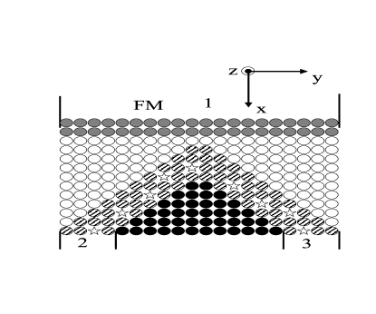
FIG. 1.: Cross section of tip-geometry shown in $xy$ plane. Gray circles denote Ferromagnetic sample, the empty circles depict vacuum, black circles corresponds to insulating sites and the rest corresponds to metallic sites(circles with downward diagonal lines) and the impurities (empty stars) in the tip.

The currents are related to potentials by

$$I_{p}=\sum_{q\neq p}G_{pq}(V_{p}-V_{q}).$$ (8)

The above expression is gauge invariant and the currents conservation law $\sum_{i}I_{i}=0$ requires that $G_{pq}$=$G_{qp}$ be satisfied.

The calculation of the conductance of the structure is based upon the non-equilibrium Green’s function formalism[11, 12]. When applied to multi-terminal ballistic mesoscopic conductor we obtain the following result for the conductance [10]

$$G_{pq}=\frac{e^{2}}{h}Tr[\Gamma_{q}G^{R}\Gamma_{p}G^{A}].$$ (9)

Here $p$ and $q$ enumerates the three terminals and the upper indices R and A refer to the retarded and advanced Green function of whole structure taking leads into account. Here $\Gamma_{p(q)}$ self-energy function for the isolated ideal leads and are given by $\Gamma_{p(q)}$=$t^{2}A_{p(q)}$, where $A_{p(q)}$ is the spectral density in the respective lead when it is decoupled from the structure. The trace is over space and spin degrees of freedom, and all the matrices in equation (4) are of size $(2N_{y}\times N_{z},2N_{y}\times N_{z})$, where $N_{y}$ and $N_{z}$ are number of sites along y and z direction and the factor 2 takes into account the spin degree of freedom. All the quantities in the above equations are evaluated at the Fermi energy. To calculate the required Green function we use the well known recursive Green function method [13].

4. Results and discussion

In this section we present numerical results for a system of cross section (20 $\times$ 20) in yz plane and a length of 10 lattice spacing along the x direction. Number of metallic layers on the tip, i.e., d in Fig.1 is taken to be 4 lattice spacings. The hopping parameter,t ,is same for all pairs and set to $-1$ for numerical calculation. The on-site energies in the leads and on the metal coating on the tip is set to be zero, while in the vacuum layer it is $\epsilon_{vac}=4.0|t|$, and in the insulating region in the tip it is $\epsilon_{ins}=10.0|t|$. The Fermi level throughout the calculation is kept fixed at $\epsilon_{f}=3|t|$ above the bottom of the band. For disorder we consider Anderson Model in which a random on-site energy, characterized by square distribution of width W, is added to the on-site energy of perfect case. In our case disorder is added only in the metallic coating on the tip; everywhere else the system is perfect.

Before we go over to the discussion of our results we briefly mention the correspondence between the physical parameters and the model parameters. The relevant physical parameters are mean-free-path, spin-relaxation length Fermi Energy and the spin polarization of the ferromagnet at the Fermi level, and the model parameters, are on-site energy, hopping energy, exchange splitting and spin-orbit coupling parameter. Physical parameters are related to the model parameters in the following way,

$$l_{m}=\frac{|t|}{\pi}\sqrt{\frac{\epsilon_{f}}{|t|}}\frac{1}{N_{3D}(\epsilon_{f})\langle(V-\bar{V})^{2}\rangle_{c}}a,$$ (10)

$$l_{so}=l_{m}\sqrt{\frac{\tau_{so}}{\tau_{m}}}\equiv\frac{3l_{m}|t|}{2|\alpha_{so}|{\epsilon_{f}}},$$ (11)

$$P=\frac{N^{\uparrow}(\epsilon_{f})-N^{\downarrow}(\epsilon_{f})}{N^{\uparrow}(\epsilon_{f})+N^{\downarrow}(\epsilon_{f})}\equiv\frac{\sqrt{\epsilon_{f}+\Delta}-\sqrt{\epsilon_{f}-\Delta}}{\sqrt{\epsilon_{f}+\Delta}+\sqrt{\epsilon_{f}-\Delta}},$$ (12)

where $l_{m}$, $l_{so}$ and P are elastic mean free path, spin relaxation length and spin polarization of the ferromagnet respectively. Here $a$ is lattice spacing and $\langle...\rangle_{c}$ represents the configuration averaging, other symbols have the same meaning as defined in the section 2. Below we present some numerical results for one typical realization of the disorder , we have not performed disorder averaging.

In Fig.2 we have plotted the conductance $G_{12}$ and $G_{13}$ as a function of magnetization angle $\theta$ with respect to z axis. We rotate the magnetization in yz plane such that the magnetization is always perpendicular to the x-axis or in other words the angle $\phi$ does not change and has fixed value of 90 degrees. To be specific, when $\theta$=0 and $\phi=90$ degrees, magnetization is parallel to $z$-axis while for $\theta$=90 and $\phi$=90 degrees the magnetization is parallel to y-axis. We have taken $\epsilon_{f}=3|t|$, $\alpha_{so}=0.02$ and $\Delta=2.4|t|$ and the Anderson disorder strength is $W=1|t|$.

FIG. 2.: Fig.2. Conductance ($G_{12}$ and $G_{13}$) versus $\theta$ plot for the two terminals for a fixed value of $\phi$=90. The other parameters chosen for this figure are $\epsilon_{f}=3.0|t|$, $\Delta=2.4|t|$, $\alpha_{so}$=0.02, and $W=1|t|$.

This set of parameters corresponds to a mean free path of $l_{m}=80a$, spin relaxation length of $l_{so}=25l_{m}$ and polarization is $P=50\%$. We notice that the conductance shows approximately cos($\theta$) as a function of angle, which is expected since in our geometry the tip is placed symmetrically to $xz$ plane. However because of disorder the effective axis in the system does not coincide with the chosen spin quantization axis, i.e., $z$ axis, and also since the structure considered is three dimensional so the scattering plane is not fixed hence the conductance variation with magnetization angle does not show an exact cosine behavior. Also we notice that the variation of $G_{13}$ is opposite to that $G_{12}$. This is in agreement with the underlying microscopic time-reversible symmetry which requires that the two terminal conductance should be symmetric under time reversal.

FIG. 3.: Plot of the average two-terminal conductance $(G_{12}+G_{13})/2$ versus $\theta$ . The other parameters are same as those in Fig.2.

To verify this point in Fig.3 we have plotted, the sum of $(G_{12}+G_{13})/2$, we see that the two terminal conductance is symmetric with respect to magnetization angle $\theta$ also the magnitude of oscillation is much smaller than either $G_{12}$ or $G_{13}$. This is due to the fact that the variation of $G_{12}$ or $G_{13}$ with $\theta$ is of first-order with respect to the spin-orbit coupling, whereas the variation of $G_{12}+G_{13}$ is of second order with respect to spin-orbit coupling. Actually the latter can be viewed as related to the anisotropic magnetoresistance of ferromagnets, whereas the former is related to the extraordinary Hall effect.

In Fig.4 we plot spin asymmetry as a function of polarization of ferromagnet for terminal 2. We have defined the spin-asymmetry as,

$$A=\frac{G^{max}_{12}-G^{min}_{12}}{G^{max}_{12}+G^{min}_{12}}$$ (13)

where to find $G^{max}_{12}$ and $G^{min}_{12}$ we generate a curve as shown in Fig.3 for each set of parameters and from those points we get the corresponding maximum and minimum values. This is necessary since the variation of conductance with magnetization angle does not follow exact cosine behavior, the maxima and minima need not to occur exactly at zero and $\pi$ respectively. we have fixed Fermi energy at $\epsilon_{f}=3|t|$ and $\alpha_{so}=0.02$. Different curves in Fig.4 corresponds to disorder strengths $W=1|t|$(solid line), $W=2|t|$(dotted line), $W=2.5|t|$ ( dot-dashed line) and $W=4|t|$ (dashed line) corresponding mean-free-paths are respectively $80a$, $10a$, $6a$, and $3a$. Although all these curves corresponds to different mean-free-paths, however the ratio $l_{so}/{l_{m}}$ is same for all the curves and is equal to 25, since this ratio is determined by Fermi energy and spin-orbit coupling strength, which are kept fixed here.

FIG. 4.: Spin asymmetry $A$, as a function of polarization for different disorder strength. The other parameters are $\epsilon_{f}=3.0|t|$ and $\alpha_{so}$=0.02.

We see that for a fixed disorder strength the spin asymmetry increases linearly with the polarization or in other words spin asymmetry is directly proportional to the polarization of ferromagnet. However for a fixed polarization value, spin asymmetry shows a non-monotonic behavior. As we increase disorder strength, spin asymmetry first increase and then starts decreasing. This shows that the spin asymmetry is maximum when the system is in quasi ballistic regime, since the multiple scattering destroys the spin asymmetry effect. Which is clearly visible in the Fig.4 where spin-asymmetry is maximum , for a fixed value of polarization, at a disorder strength $W=2|t|$ ,corresponding to a mean-free-path of $10a$, while it is minimum for $W=4|t|$ corresponding to a mean-free-path of $3a$ lattice spacings. The order of magnitude of spin-asymmetry is $5\%$, which is in good agreement with the prediction in Ref.[7].

In Fig.5 we have studied the behavior of spin asymmetry as a function of spin-orbit coupling parameter $\alpha_{so}$. The other parameters are same as in Fig.4. We notice that the spin-asymmetry shows a linear behavior for small values of $\alpha_{so}\leq 0.03$, for larger $\alpha_{so}$ the linear behavior is no longer seen, because for a fixed disorder, i.e., fixed $l_{m}$, as we increase $\alpha_{so}$, correspondingly , $l_{so}$ , i.e. spin-relaxation path decreases, hence the higher order effect in spin-orbit coupling starts dominating so we no longer observe a linear behavior. Also we see that for a fixed $\alpha_{so}$, spin-asymmetry shows a maximum at a disorder strength of around $W=2|t|$. This is in harmony with the results presented in Fig.4. The typical value of spin asymmetry is of the order of $5\%$. So from the results of Fig.4 and Fig.5 we can say with confidence that the efficency of the proposed three terminal STM device would be maximum when the device operates in quasi-ballistic regime.

FIG. 5.: Spin asymmetry $A$, as a function of $l_{m}/l_{so}$ for different disorder strength. The other parameters are $\epsilon_{f}=3.0|t|$ and $\Delta=2.4|t|$ corresponding value of polarization is 50$\%$.

In summary we have developed a new model to take into account spin- orbit scattering within the single-band tight-binding model. Using this model we have done numerical calculation of magnetic scanning tunneling microscopy with a non-magnetic tip. The order of magnitude of the spin-asymmetry is about $5\%$, which is in good agreement with the qualitative estimate given in [7], and the effect is maximum when the device operates in the quasi-ballistic regime. The spin-asymmetry of the present effect is smaller than the one obtained in the spin-valve tunneling structures. However, it has some advantages. In particular since the tip is non-magnetic, it is insensitive to an external magnetic field . This allows one to study the domain structure as function of applied field. Furthermore, the problem of the magnetostatic interaction between the tip and the magnetic sample is avoided, which incase of a magnetic tip would give rise to undesirable magnetic forces between the tip and the sample and are likely to influence the domain structure. Another important advantages of this technique is that by measuring separately the currents $I_{2}$ and $I_{3}$ of the two tip terminals, and by combining them appropriately, one can separate the weak magnetic contrast from the dominant topographic contrast: the sum $I_{2}+I_{3}$ depends only on the topography, whereas the magnetic information is contained in the difference $I_{2}+I_{3}$. Besides all these advantages it has an intrinsic limitation that the only in-plane components can be studied and also since multiple scattering diminishes the spin-asymmetry effect, it is necessary that the device operates in a quasi-ballistic regime. However to construct such a tip would be experimentally challenging.

REFERENCES

- [1] M. Juliere, Phys. Lett. 54A, 225 (1975); S. Maekawa and U. Gäfvert, IEEE Trans. Magn. 18, 707 (1982); J. C. Slonczewski, Phys. Rev. B 39 6995 (1989).
- [2] R. Wiesendanger, H. J. Güntherodt, G. Güntherodt, R. J. Gambino, and R. Ruf, Phys. Rev. Lett. 65, 247 (1990);R. Wiesendanger, J. Magn. Soc. Jpn. 18, 4(1994).
- [3] W. Wulfhekel and J. Kirschner, App. Phys. Lett. 75,1944 (1999).
- [4] S. Heinze, M. Bode, A. Kubetzka, O. Pietzsch, X. Nie, S. Blügel and R. Wiesendanger, Science 288, 1805 (2000).
- [5] O. Pietzsch , A Kubetzka, M. Bode, and R. Wiesendanger, Phys. Rev. Lett. 84 5212 (2000).
- [6] M. Bode, M. Getzlaff, R. Wiesendanger, Phys. Rev. Lett. 81 4256 (1998).
- [7] P. Bruno, Phys. Rev. Lett. 79, 4593 (1997)
- [8] N. F. Mott, Proc. R. Soc. London A 124, 438 (1929).
- [9] M. Büttiker, Phys. Rev. Lett. 57, 1761 (1986); IBM J. Res. Dev. 32 317 (1988).
- [10] S. Datta, Electronic Transposrt in Mesoscopic Systems (Cambridge University Press, Cambridge 1995).
- [11] L.P. Kadanoff, G. Baym, Quantum Statistical Mechanics, Benjamin, New Yeak, 1962.
- [12] L.V. Keldysh, Soviet Phys. JETP 20 (1965) 1018.
- [13] H. U. Baranger, D. P. DiVincenzo, R. A. Jalabert, and A. D. Stone, Phys. Rev. B 44, 10637 (1991).