Modeling Two-Roton Bound State Formation in Fractional Quantum Hall System

Abstract

Composite Fermion approach using extensive and parallelized numerical analysis has recently established a two-roton bound state as the lowest energy long wavelength neutral excitation of fractional quantum Hall effect for finite particle ($N\sim~{}30$ ) system. By focusing on the oriented dipole character of magneto roton, we model the two roton problem and solve it variationally (analytically) to find a two roton bound state with binding energy which is in good agreement with the composite Fermion numerical results.

The pioneering work of Girvin, Macdonald and Platzman (GMP) [1] brought out non-trivial inner structure of neutral excitations of the Fractional Quantum Hall Effect (FQHE) [2] systems. This inner structure is very transparent for the magneto roton, the minimum energy neutral excitations at a finite wave vector $k_{0}l_{0}=1.4$ for the $\nu=\frac{1}{3}$ quantum Hall state. They are well approximated by a Laughlin quasi-hole ($\frac{e}{m}$) - quasi-particle ($-\frac{e}{m}$) bound state, as shown in Fig. 1a. The composite Fermion (CF) [3] approach, that goes beyond Laughlin hierchy of $\frac{1}{m}$ filling, views the neutral excitations as a composite Fermion interband excitons of the ‘pseudo’ Landau bands. The CF approach has also suggested variational schemes that is amenable to numerical studies. Theoretical studies of neutral excitations have become meaningful in the light of the Raman scattering experiments [4]- [5].

The aim of the present Letter is to provide an effective microscopic model that uses the essential structure of magneto roton. In our parameter free theory we get the two-roton ( with zero total momentum ) binding energy that is in good agreement with the extensive finite particle system study result in the CF approach. We first show that the magneto roton is an $oriented$ $dipole$ analogous to the description of a magnetic exciton [6], [7], [8] as well as Read’s [9] dipole description of the neutral composite fermion at $\nu=\frac{1}{2}$. The dipole moment vector ( $\vec{d}$ ), the momentum of the magneto roton ($\vec{p}$ ) and the external magnetic field ($\hat{z}$ ) form a triad $(\hat{z}=\frac{\vec{d}\times\vec{p}}{|\vec{d}||\vec{p}|}$). The oriented character of the dipole moment leads to a velocity dependent effective interaction between two rotons, analogue to the velocity dependent interaction found by one of the author’s [10], in the context of BCS instability of composite Fermi liquid. The resulting two body problem is solved variationally to find a bound state. The binding energy of our ( parameter free ) theory is in good agreement with the numerical results of Park and Jain [11].

In the single mode approximation ( SMA ) a neutral excitation is defined by (unnormalized) wave function $\psi_{q}=P_{LLL}\rho_{q}\psi_{L}$ , where $\rho_{q}=\sum_{i}e^{i\vec{q}.\vec{r}_{i}}$. The minimum of energy $(E_{min}=E_{rot})$ occurred at $k=k_{0}$ and this excitation was called magneto roton, by analogy with roton of liquid ⁴helium [12].

It was observed by GMP [1] that the zero momentum neutral excitation, as observed by numerical experiment [13] was in disagreement with their result at E($k=0$). Since the numerically observed results was slightly less than $2E_{rot}(k=k_{0})$, they speculate that the minimum energy excitation could be a two-roton bound state, as shown in Fig. 1b. Within the Landau-Ginzburg theory, Lee and Zang [14] also proposed that the $k=0$ excitation consists of two dipoles (two magneto-rotons ), arranges in such a way that it has quadrupole moment but the net dipole moment is zero. Two-roton bound state are suspected to occur in liquid ⁴helium [16].

In a recent paper, Park and Jain [11] have extended their CF exciton theory of magneto roton to two-roton bound state problem. Using parallel computing technique, they have handled upto 30 particle systems. They have shown very convincingly that the zero momentum lowest energy excitations is a two-roton bound state.

According to Laughlin [15], the elementary charged excitations, at the filling fraction $\nu=\frac{1}{m}$, are quasiparticles (q.p) and quasiholes (q.h) with fractional charge $\pm\frac{e}{m}$. The effective magnetic length for a particle with fractional charge $\frac{e}{m}$ is $l_{0}\sqrt{m}$, where $l_{0}=\sqrt{\frac{\hbar c}{eB}}$ is the magnetic length for a particle with charge e. A roton with wave vector $|\vec{k}|$ is a bound state of a q.p and q.h separated by a large distances $mkl_{0}^{2}$. A q.p and q.h have an attractive Coulomb interaction $V(\vec{r})=-\frac{e^{2}}{m^{2}\epsilon r}$. In lowest Landau level at filling fraction $\nu=\frac{1}{m}$ ( m is an odd integer), they obey the following guiding center dynamics [9], [10]:

$$\frac{d\vec{r}_{e}}{dt}=\frac{ml_{0}^{2}}{\hbar}\nabla_{e}V(\vec{r}_{e}-\vec{r}_{h})\times\hat{z}$$ (1)

$$\frac{d\vec{r}_{h}}{dt}=-\frac{ml_{0}^{2}}{\hbar}\nabla_{h}V(\vec{r}_{e}-\vec{r}_{h})\times\hat{z}$$ (2)

where $\vec{r}_{e}$ and $\vec{r}_{h}$ are the co-ordinates of the q.p and the q.h. These equation leads to a drift velocity $\vec{v}_{d}=\frac{d}{dt}\vec{R}$ of the center of mass of the pair:

$$\vec{v}_{d}=\frac{ml_{0}^{2}}{\hbar}(\nabla_{\vec{r}}V(\vec{r})\times\hat{z})$$ (3)

where $\vec{r}=\vec{r}_{e}-\vec{r}_{h}$ is the relative distance between the q.p and q.h. and $\vec{R}=\frac{(\vec{r}_{e}+\vec{r}_{h})}{2}$ center of mass co-ordinate. Since the q.p and q.h carry opposite charges, they both drift in a direction perpendicular to their separation vector ${\vec{r}}$ direction.

$$\vec{r}.\vec{v}_{d}=\frac{ml_{0}^{2}}{\hbar}\vec{r}.(\nabla_{\vec{r}}V(\vec{r})\times\hat{z})=\frac{ml_{0}^{2}}{\hbar}\hat{z}.(\vec{r}\times\nabla_{\vec{r}}V(\vec{r}))=0,$$ (4)

since $\vec{r}\times\nabla_{\vec{r}}V(\vec{r})$ is zero. Hence $\vec{r}.\vec{v}_{d}=0$. Laughlin’s quasi-exciton wave function ( see Eq. (8) of Ref. [7]) can be re-written in terms of the center of mass and the relative co-ordinates as

$$|z_{0}> = \frac{1}{\sqrt{2mL}}\int\int e^{i\vec{R}.(\vec{k}+\frac{\vec{r}\times\hat{z}}{2ml_{0}^{2}})}e^{-\frac{|\vec{r}-ml_{0}^{2}\hat{z}\times\vec{k}|^{2}}{4ml_{0}^{2}}}$$ (6)

$$S_{z_{e}}^{{\dagger}}S_{z_{h}}|m>d^{2}z_{e}d^{2}z_{h}$$

The amplitude of this wave function is maximum when $\vec{r}=ml_{0}^{2}\vec{k}\times\hat{z}$. So Laughlin’s quasi-exciton wave function strongly suggest the oriented nature of our dipole. This dipole dynamics is very similar to the dynamics of a vortex anti-vortex in fluid dynamics. The distance between the constituent particles of a roton ( oriented dipole ) is $\vec{r}=ml_{0}^{2}(\hat{z}\times\vec{k})$. The dipole moment of this roton is $\vec{d}=\frac{e}{m}ml_{0}^{2}(\hat{z}\times\vec{k})$ or $\vec{d}=el_{0}^{2}(\hat{z}\times\vec{k})$. The dipole moment is the same for $\nu=\frac{1}{3}$ and $\nu=\frac{1}{2}$ for a given $\vec{k}$.

At filling fraction $\nu=\frac{1}{m}$, there is a parabolic dispersion around the minimum energy at finite $k=k_{0}$. The energy spectrum can be written around the minimum energy at $k=k_{0}$ as

$$E(k)=E_{rot}+\frac{\hbar^{2}}{2m_{r}}(|\vec{k}|-k_{0})^{2},$$ (7)

where $E_{rot}$ is the minimum roton energy at $k=k_{0}$ and $m_{r}$ is the roton mass. The minimum roton energy $E_{rot}$ and the corresponding $k_{0}$ are different for different filling fractions. So the kinetic energy of a roton is different for different filling fractions through $m_{r}$ and $k_{0}$. For $\nu=\frac{1}{3}$, $E_{rot}=0.075\frac{e^{2}}{\epsilon l_{0}}$ is the minimum roton energy at $k_{0}l_{0}=1.4$. $m_{r}=2\epsilon\hbar^{2}/e^{2}l_{0}$ is the roton mass. The mass of a roton is calculated from the curvature of the excitation spectrum at $\nu=\frac{1}{3}$ given in Ref. [1] by using the relation $m_{r}=\frac{\hbar^{2}}{\frac{\partial^{2}E(k)}{\partial k^{2}}}$ at $k=k_{0}$.

The kinetic energy for two roton with momenta $\vec{k}_{1}$ and $\vec{k}_{2}$ is

$$T=\frac{\hbar^{2}}{2m_{r}}[(|\vec{k}_{1}|-k_{0})^{2}+(|\vec{k}_{2}|-k_{0})^{2}].$$ (8)

Since each roton is an $oriented$ $dipole$, it is a natural choice to consider the interaction between two roton as a dipole-dipole interaction. This momentum dependent dipole-dipole interaction was first suggested by one of the author’s [10] for $\nu=\frac{1}{2}$ composite Fermi liquid. The classical dipole-dipole interaction energy with two dipoles $\vec{d}_{1}$ and $\vec{d}_{2}$ is,

$$U=\frac{\vec{d}_{1}.\vec{d}_{2}}{\epsilon r_{12}^{3}}-3\frac{(\vec{d}_{1}.\vec{r}_{12})(\vec{d}_{2}.\vec{r}_{12})}{\epsilon r_{12}^{5}},$$ (9)

where $\vec{r}_{1}$ and $\vec{r}_{2}$ are the position vectors of the two dipoles and $\vec{r}_{12}=\vec{r}_{1}-\vec{r}_{2}$ is the relative distance between two dipoles. $\epsilon$ is the dielectric constant of the background material.

$\vec{d}_{1}=el_{0}^{2}(\hat{z}\times\vec{k}_{1})$ and $\vec{d}_{2}=el_{0}^{2}(\hat{z}\times\vec{k}_{2})$ are the dipole moments of the two roton with wave vector $\vec{k}_{1}$ and $\vec{k}_{2}$ respectively and $|\vec{r}_{12}|$ is the relative distance between two rotons. Using the dipole moments $\vec{d}_{1}$ and $\vec{d}_{2}$ for the two rotons, this interaction energy can be rewritten in terms of the total momentum $\vec{K}=\vec{k}_{1}+\vec{k}_{2}$ and relative momentum $\vec{k}=\vec{k}_{1}-\vec{k}_{2}$ as

$$U=\frac{e^{2}l_{0}^{4}}{4\epsilon}[\frac{(\vec{K}^{2}-\vec{k}^{2})}{r_{12}^{3}}-3\frac{(\hat{z}\times(\vec{K}+\vec{k}).\vec{r}_{12})(\hat{z}\times(\vec{K}-\vec{k}).\vec{r}_{12})}{r_{12}^{5}}]$$ (10)

This is a semi classical expression for the potential energy of two interacting oriented dipoles . Since an oriented dipole is a quantum mechanical particle, we pass on to quantum dynamics by symmetrize the above classical energy expression and replace the total momentum $\vec{K}$ and the relative momentum $\vec{k}$ by an operator $-i\nabla_{\vec{R}}$ and $-i\nabla_{\vec{r}}$ respectively. After symmetrize, interaction energy reduces to

$$U = \frac{e^{2}l_{0}^{4}}{4\epsilon}[\frac{\vec{K}^{2}}{r_{12}^{3}}-\frac{1}{r_{12}^{3}}\vec{k}^{2}-\vec{k}^{2}(\frac{1}{r_{12}^{3}})$$ (11)

$$- 3\frac{(\hat{z}\times\vec{K}).\vec{r}_{12}(\hat{z}\times\vec{K}).\vec{r}_{12}-(\hat{z}\times\vec{k}).\vec{r}_{12}(\hat{z}\times\vec{k}).\vec{r}_{12}}{r_{12}^{5}}]$$ (12)

In operator form, it becomes

$$U = \frac{e^{2}l_{0}^{4}}{4\epsilon}[\frac{-\nabla_{\vec{R}}^{2}}{r_{12}^{3}}+\frac{1}{2}(\frac{1}{r_{12}^{3}}\nabla_{\vec{r}}^{2}+\nabla_{\vec{r}}^{2}(\frac{1}{r_{12}^{3}}))-\frac{3}{r_{12}^{5}}\frac{\partial^{2}}{\partial\phi^{2}}$$ (13)

$$+ \frac{3}{r^{3}}(\sin^{2}(\theta+\phi)\frac{\partial^{2}}{\partial R^{2}}+\cos^{2}(\theta+\phi)\frac{1}{R^{2}}\frac{\partial^{2}}{\partial\theta^{2}}$$ (14)

$$+ \cos^{2}(\phi-\theta)\frac{1}{R}\frac{\partial}{\partial R}+\sin 2(\phi-\theta)\frac{1}{R^{2}}\frac{\partial}{\partial\theta})],$$ (15)

where $\phi$ is the angle between $\vec{r}$ and $x$ axis and $\theta$ is the angle between $\vec{R}$ and $X$ axis. The term $\frac{1}{2}(\frac{1}{r_{12}^{3}}\nabla_{\vec{r}}^{2}+\nabla_{\vec{r}}^{2}(\frac{1}{r_{12}^{3}}))$ in the above expression is due to symmetrization of $\frac{\nabla_{\vec{r}}^{2}}{r_{12}^{3}}$ term. Without symmetrization of this term $\frac{\nabla_{\vec{r}}^{2}}{r_{12}^{3}}$, the interaction does not give the correct binding energy. So quantum mechanics play a crucial role in the interaction between two rotons. This is a momentum dependent, non-central potential between two oriented dipoles of non-zero total momentum. This momentum dependent interaction energy is same for all $\nu=\frac{p}{(2mp+1)}$ filling fractions, where $m$ and $p$ are integers.

Since we are interested in the pair formation, we concentrate only two roton with opposite momenta ($\vec{k}_{1}=-\vec{k}_{2}$), as done in BCS theory. Hence the total momentum is zero. The interaction energy can be written as

$$U=\frac{e^{2}l_{0}^{4}}{4\epsilon}[\frac{1}{2}(\frac{1}{r_{12}^{3}}\nabla_{\vec{r}}^{2}+\nabla_{\vec{r}}^{2}(\frac{1}{r_{12}^{3}}))-\frac{3}{r_{12}^{5}}\frac{\partial^{2}}{\partial\phi^{2}}].$$ (16)

The Hamiltonian for this two body problem with the total momentum $\hbar\vec{K}=0$ becomes

$$H = \frac{\hbar^{2}}{4m_{r}}(|i\vec{\nabla}_{\vec{r}}|-2k_{0})^{2}$$ (17)

$$+ \frac{e^{2}l_{0}^{4}}{4\epsilon}[\frac{1}{2}(\frac{1}{r_{12}^{3}}\nabla_{\vec{r}}^{2}+\nabla_{\vec{r}}^{2}(\frac{1}{r_{12}^{3}}))-\frac{3}{r_{12}^{5}}\frac{\partial^{2}}{\partial\phi^{2}}].$$ (18)

We propose a variational wave function

$$\psi(r)=Nr^{2}e^{-\alpha r}J_{0}(2k_{0}r),$$ (19)

where N is the normalization constant which is determined by the condition $\int d^{2}r|\psi(r)|^{2}=1$, $J_{0}(2k_{0}r)$ is the zeroth order Bessel function and $r=|\vec{r}_{12}|$. $\alpha$ is the variational parameter which can be determined by minimizing the energy expectation value.

In superconductivity, Cooper pair forms at the Fermi surface between two electrons with opposite momenta. Similarly, roton pair forms at and near $k=k_{0}$. The annular region in k-space that contributes to $\vec{K}=0$ magneto roton bound state is shown in Fig.2. Like Cooper pair wave function, we construct a wave function for the two-roton bound state with momenta ($\vec{k}_{0},-\vec{k}_{0}$) which gives $J_{0}(2k_{0}r)$ for s-state. $2k_{0}$ is the relative momentum of these two roton.

To calculate the expectation value of the first term
( kinetic term ) on the right hand side of this Hamiltonian, we go to the momentum space. The variational wave function in momentum space is

$$\psi(k)=N^{\prime}\frac{6}{\alpha^{4}}\int_{0}^{2\pi}d\theta F[2,2.5;1;-\frac{(k^{2}+4k_{0}^{2}-4kk_{0}\cos\theta)}{\alpha^{2}}]$$ (20)

where $N^{\prime}$ is the normalization constant. In momentum space the kinetic energy operator is $T=\frac{\hbar^{2}}{4m}(k-2k_{0})^{2}$. The expectation value of the kinetic energy in k-space is $E_{1}(\tilde{\alpha})=0.125E_{c}\int d^{2}\tilde{k}|\psi(\tilde{k})|^{2}(\tilde{k}-2.8)^{2}$, where $E_{c}=\frac{e^{2}}{\epsilon l_{0}}$ is the unit of Coulomb energy and $\tilde{\alpha}=\alpha l_{0}$ and $\tilde{k}=kl_{0}$ are the dimensionless variables.

The expectation value of the interaction term ( second term of the Hamiltonian ) is $E_{2}(\tilde{\alpha})=\frac{0.125B}{A}E_{c}$ where A and B are the following integrals:

$$A=\int_{0}^{\infty}d\tilde{r}\tilde{r}^{5}(J_{0}(2.8\tilde{r}))^{2}e^{-2\tilde{\alpha}\tilde{r}},$$ (21)

$$B=\int_{0}^{\infty}d\tilde{r}[4-2\tilde{r}^{2}\tilde{\alpha}^{2}+2\tilde{\alpha}\tilde{r}-15.68\tilde{r}^{2}]J_{0}^{2}(2.8\tilde{r})e^{-2\tilde{\alpha}\tilde{r}}.$$ (22)

We are numerically minimizing the energy functional $E(\tilde{\alpha})=E_{1}(\tilde{\alpha})+E_{2}(\tilde{\alpha})$ with respect to the variational parameter $\tilde{\alpha}$. The minimum energy for two-roton state is 0.138 $E_{c}$ at $\tilde{\alpha}=0.41$ whereas $2E_{rot}=0.15E_{c}$ so that the binding energy is $0.012E_{c}$. Park and Jain have found a minimum energy of 0.135 $E_{c}$ and hence the binding energy is 0.015 $E_{c}$. Our binding energy is thus in good agreement with the extensive numerical results of Park and Jain [11]. So two rotons with opposite momenta forms a bound state.

The root mean square distance between these two roton is $\sqrt{<r^{2}>}\sim 6.7l_{0}$ where as the size of a single roton is approximately 4.2 $l_{0}$.

When the total momentum $\vec{K}$ of a two-roton bound state increase, the energy is also increased. At $K\geq K_{c}$, the two-roton bound state breaks into two rotons. To get a qualitative idea that how the excitation spectrum of a bound state goes with the total momentum, we use semiclassical approximation. We consider $\vec{k}_{1}=\vec{k}_{0}+\vec{q}$ and $\vec{k}_{2}=-\vec{k}_{0}$, where $|\vec{q}|<|\vec{k}_{0}|$. One can easily get the semiclassical energy $E(K)=E_{c}[0.3125(Kl_{0})^{2}-0.01(1+0.77(Kl_{0})^{2})]$ The critical momentum $K_{c}$ can be determined by the condition, $E(K=0)+E(K)=2E_{rot}$. Using this condition, we have $K_{c}l_{0}=0.22$. The two-roton bound state is not the lowest energy excitation when $K\geq K_{c}$. Expected excitation spectrum of a two-roton bound state and the two roton continuum state is shown in Fig. 3. and compared with a single roton excitation spectrum which is given in Ref. [1]. The effective mass of a two roton bound state is $M=0.054m_{e}$ which is 75 percent less than the sum of the two rotons mass.

In conclusion, we identified the magneto roton as an oriented dipole. We derived the momentum dependent, non-central interaction energy form between two rotons from a classical dipole-dipole interaction energy. Finally we proposed a wave function for two-roton state and shown analytically that at $\nu=\frac{1}{3}$ lowest energy excitation is a two-roton bound state (with zero total momentum) instead of a single roton.

One of us (G.B) wish to thank Steve Girvin for a discussion. This research was supported in part by the National Science Foundation under Grant No. PHY94-07194.

FIG. 1.: Schematic diagrams for ( a ) a single roton with momentum $\vec{k}_{o}$ and ( b ) a two-roton bound state with total momentum $\vec{K}=0$.

FIG. 2.: Annular region in k-space that contributes to $\vec{K}=0$ magneto-roton bound state.

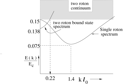
FIG. 3.: Expected qualitative excitation spectrum of two-roton bound state compared with excitation spectrum of a single roton.

REFERENCES

• [1] S. M. Girvin, A. H. Macdonald, and P. M. Platzman, Phys. Rev. Lett. 54, 581 (1985); Phys. Rev. B 33 , 2481 (1986).
• [2] D. C. Tsui, H. L. Stormer and Gossard, Phys. Rev. Lett. 48, 1559 (1982).
• [3] J. K. Jain, Phys. Rev. Lett. 63, 199 (1989); Phys. Rev. B 41, 7653 (1990).
• [4] M. Kang, A. Pinczuk, B. S. Dennis, M. A. Eriksson, L. N. Pfeiffer, and K. W. West, Phys. Rev. Lett. 84, 546 (2000).
• [5] H. D. M. Davies, J. C. Harris, J. F. Ryan, and A. J. Turberfield, Phys. Rev. Lett. 78, 4095 (1997).
• [6] Yu. A. Bychkov, S. V. Iordanskii and G. M. Eliashberg, Sov. Phys. JETP Lett. 33, 143 (1981)
• [7] R. B. Laughlin, Physica B, 126, 254 (1984).
• [8] C. Kallin and B. I. Halperin, Phys. Rev. B 30, 5655 (1984).
• [9] N. Read, Semi. Sci. Tech. 9 , 1859 (1994); Surf. Sci. 361/362, 7 (1996).
• [10] G. Baskaran, Physica B, 212, 320 (1995).
• [11] K. Park and J. K. Jain, Phys. Rev. Lett. 84, 5576 (2000).
• [12] R. P. Feynman, Statistical Mechanics (Benjamin, reading, Mass, 1972); Phys. Rev. 91, 1291, 1301 (1953); 94, 262, (1954); R. P. Feynman and M. Cohen, ibid. 102, 1189 (1956).
• [13] F. D. M. Haldane and E. H. Rezayi, Phys. Rev. Lett. 54, 237 (1985).
• [14] D. H. Lee and S. C. Zang, Phys. Rev. Lett, 66 , 1220 (1991).
• [15] R. B. Laughlin, Phys. Rev. Lett. 50, 1395, (1983).
• [16] A. Zawadowski, J. Ruvalds, and J. Solana, Phys. Rev. A 5, 399 (1972); V. Celli, and J. Ruvalds, Phys. Rev. Lett. 28, 539 (1972).
Refer to caption