Spectrum and thermodynamic currents in one-dimensional Josephson elements

Abstract

The dc Josephson effect is considered from the thermodynamic point of view. Universal thermodynamic equations, relating both bound and continuum contributions to the Josephson current with the normal electron scattering amplitudes are derived for the single mode case. To derive these equations we use and further develop the method of spatial separation between the superconducting and normal parts of the junction. We also use this method to find the Andreev bound states in structures containing superconducting components. The general thermodynamic formulas are applied to the calculation of the current in various Josephson-type structures. In particular, the crucial role of the continuum contribution is demonstrated, even for short junctions (where it is usually neglected). We also find structures where the bound states supporting the giant currents are well separated; thus they can, hopefully, be populated nonuniformly and such current can be measured.

I Introduction

Numerous theoretical investigations of Josephson junctions show that the equilibrium nondecaying current can be expressed in terms of a quasiparticle description based on Bogolubov-de Gennes (BdG) equations. There are two contributions to the current: one is supported by discrete states lying within the superconductor gap (so called “bound” current); and the other, carried by continuum of propagating modes outside the gap (“continuum” current). Most authors find the bound contribution from the thermodynamic relation

$$I=\frac{2e}{\hbar}\frac{dF}{d\varphi}$$ (1)

where $F$ is the free energy of the system and $\varphi$ is the superconductor phase difference across the junction, while the continuum one is found from a Landauer type consideration which yields a current resulting from imbalance of left-going and right-going quasiparticle fluxes (it is non-zero in the superconductors).

A more general method, allowing to obtain both discrete and continuum contributions from the thermodynamic approach was suggested by Beenakker [1]. He derived the following expression for the free energy:

$$F=-2k_{B}T\sum_{E_{n}>0}\ln\left[2\cosh\frac{E_{n}}{2k_{B}T}\right]+const.$$ (2)

where “$const.$” represents the $\varphi$–independent term, canceling the divergence of the first term at high energies. The only significant approximation made in the derivation of this formula is the steplike pair-potential shape:

$$\Delta(x)=\left\{\begin{array}[]{lll}\Delta_{0}e^{-i\varphi/2}&\mbox{if}&x<-L/2,\\ 0&\mbox{if}&|x|<L/2,\\ \Delta_{0}e^{i\varphi/2}&\mbox{if}&x>L/2\end{array}\right.$$ (3)

where $L$ is the junction length. The applicability of this model was discussed previously [1, 2, 3]. The important conditions for applicability of this model are: (i) Existence of a high barrier on the boundary of the superconducting and normal media. (ii) Low current, such as $\hbar e\rho_{s}/(mJ_{Q})$ (where $J_{Q}$ is the current density and $\rho_{s}$ — the superconducting density) to be much greater than all characteristic lengths such as coherence length, junction width, etc. The superconductor - semiconductor - superconductor and superconductor - insulator - superconductor junctions usually belong to this category.

The expression for the Josephson current follows directly from Eqs. (1) and (2):

$$I_{J} \equiv I_{b}+I_{c}=-\frac{2e}{\hbar}\sum_{0<E_{n}<\Delta}\tanh\frac{E_{n}}{2k_{B}T}\;\frac{dE_{n}}{d\varphi}$$ (5)

$$-\frac{2e}{\hbar}2k_{B}T\int_{\Delta}^{\infty}dE\,\ln\left[2\cosh\frac{E}{2k_{B}T}\right]\,\frac{d\rho}{d\varphi}$$

where $\rho$ is the continuum density of states [1]. The first term of Eq. (5) is the well known bound state current[4, 5, 6] while the second term represents the continuum contribution. It requires the knowledge of the dependence of the continuum density of states (DOS) on $\varphi$. An important tool, providing this information is Krein’s theorem[7] (see Appendix A), that connects the change in the DOS induced by any scatterer with the corresponding scattering matrix.

Using this theorem, Beenakker[1] expressed the continuum contribution via the scattering matrix of the normal electrons in the multichannel case. We are going to specialize this approach to one-dimension (1D) case developing the simplified expressions for this special case. Below we consider a general junction, consisting of an arbitrary one-dimensional (1D) nonsuperconducting constriction (barrier) sandwiched between two superconductors. The relevant scattering matrix has the dimensions $4\times 4$ and it can be expressed in terms of the energy-dependent normal electron S-matrix and the scattering amplitudes on the $NS$ boundaries.

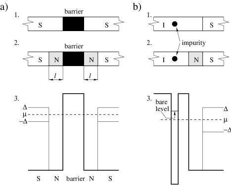
FIG. 1.: (a) General $S-barrier-S$ and (b) $I-impurity-I-S$ structures. (1) Geometric outline of the real problem. (2) Our model problem. (3) The energy diagram in the latter case. Thick line represents the potential $V(x)$, thin line: the pair potential, dashed line: the electro-chemical potential.

II Spatial separation of the superconductors from the barrier

In the next sections we express the bound spectrum and the Josephson current in a superconductor/general nonsuperconducting constriction/superconductor (SCS) junction via the scattering matrix of normal electrons. To do so we insert a fictitious ideal clean normal leads of length $l$ between the superconductors and the constriction[1] [Fig. 1($a$)]. The propagation of electrons in the “normal” medium is described by the model Hamiltonian

$$H_{0}=-\frac{\hbar^{2}}{2m}\nabla^{2}-\mu+V.$$ (6)

Below we consider the limit $l\rightarrow 0$. Beenakker[1], when inserting the fictitious normal metal, demanded that its size is smaller than all lengths in the system except the Fermi wavelength, since in this case, he claimed, the normal metal insertion does not affect the results. This is true in the zero order in $\Delta/\mu$ (Andreev approximation). Some of our calculations are done beyond the Andreev approximation, and in this case one must take the length of the normal metal to be shorter than the Fermi wavelength. This would appear meaningless from the physical point of view. However, we adopt the formal point of view, and consider the “normal metal” as a domain in the BdG equation in which the external potential and the order parameter are both zero. We then can take this domain to be shorter than the Fermi wave length. On the other hand, the scattering formulation is still valid even when the normal-metal length is infinitesimally small because in one dimension the outgoing wavefunction takes its asymptotic form $\propto e^{ikx}$ at any distance from the barrier, however small it is, since there are no evanescent modes in the 1D case.

Below we demonstrate that our results for the energy spectrum, persistent currents (when exist), reflection amplitudes etc. for arbitrary structures with fictitious normal layers agree with the corresponding results for analogous structures without these layers obtained previously using different methods[6, 8, 9] both under Andreev approximation (Appendix B) and beyond it (Sec. III). This is to be expected, since the insertion of the fictitious normal metal corresponds to a non-singular perturbation and it does not influence the results in the limit $l\rightarrow 0$.

Where the Andreev approximation is used, it is convenient to set the Fermi momentum in the normal and superconducting leads to be equal. In this case one can neglect the normal reflection at the $NS$ boundaries [8].

III Bound States in the $INIS$ junction

To illustrate the spatial separation method we consider the formation of the bound states in the insulating-superconducting structure containing an ”impurity” embedded in the insulating region. By impurity we mean a quasi-bound state of energy $E_{0}$ and width $\Gamma$ that would be formed in analogous system where the superconductor is replaced by a normal metal. Such a situation takes place, for instance, in the $INIS$ junction [Fig. 1($b$)]. An analogous problem has been considered by Laikhtman in terms of the tunneling Hamiltonian approximation[10]. It was found that there exists a single bound state in this system, whose energy can be found from the equation:

$$E^{2}_{0}+\Gamma^{2}-E^{2}=\frac{2\Gamma E^{2}}{\sqrt{\Delta^{2}-E^{2}}}.$$ (7)

In the limit $\Gamma\rightarrow 0$ the energy $E$ of this state tends to $E_{0}$ if $-\Delta<E_{0}<\Delta$. On the other hand, using more exact wavefunction matching method it was shown[6] that there exists a bound state of energy close to $\Delta$ at an $IS$ boundary without impurity.

We consider the following problem: An impurity with energy $E_{0}$, $-\Delta<E_{0}<\Delta$ located at a distance $L$ from the superconductor. Using the spatial separation method we find two energy levels: one close to $E_{0}$ and one close to $\Delta$ for the case of large $L$ (small $\Gamma$). The level close to $\Delta$ can not be obtained using the tunneling Hamiltonian method.

In order to find the bound states in this structure we insert a fictitious infinitesimally short normal layer between the superconductor ($S$) and the rest of the structure ($R$). Consider the motion of the quasiparticle in the normal layer. The quasiparticle can be either normal or Andreev reflected at the $NS$ boundary and only normal reflected at the $RN$ boundary (see Fig. 2).

FIG. 2.: Formation of a bound state on $RS$ boundary. Solid and dashed arrows represent the electron and the hole propagation correspondingly. Amplitudes $a_{e(h)},b_{e(h)}$ illustrate the Andreev and normal reflection amplitudes for electrons (holes) on $NS$ boundary; $r^{\prime}_{e(h)}$: the normal reflection on $RS$ boundary (prime indicates that the reflected particle moved initially to the left), numbers enumerate the scattering channels.

From the uniqueness of the wave function one obtains the eigenenergy equation:

$$\det\left[\left(\begin{array}[]{cc}b_{e}&a_{h}\\ a_{e}&b_{h}\end{array}\right)\left(\begin{array}[]{cc}r^{\prime}_{e}&0\\ 0&r^{\prime}_{h}\end{array}\right)-1\right]=0.$$ (8)

In the case that $R$ contains an impurity we assume that the reflection amplitude of electrons (holes) at energies close to the bare impurity level take the form

$$r_{e}(E)=r_{0}(E)\frac{E-E_{0}-i\Gamma}{E-E_{0}+i\Gamma};\;r_{h}(E)=r^{*}_{e}(-E)$$ (9)

that contains both a Breit-Wigner-type resonance and a slow energy dependence $r_{0}(E)$ as in Eq. (10) below. Note, that $|r_{e}|=1$ since there are no propagating modes within the insulator. Substituting these reflection amplitudes to Eq. (8), neglecting the energy dependence of $r_{0}$ and using the Andreev approximation which provides $b_{e}=b_{h}=0;\;a_{e}=a_{h}=v_{0}/u_{0}$ [where $u_{0}$ and $v_{0}$ are the BCS coherence factors: $u_{0}^{2}=(1+\sqrt{1-\Delta^{2}/E^{2}})/2$, $v_{0}^{2}=(1-\sqrt{1-\Delta^{2}/E^{2}})/2$], one obtains Eq. (7) which has only one positive energy solution. Taking into account the energy dependent $r_{0}(E)$ is crucial for obtaining the second level.

The numerical solution of Eq. (8) for the case $\mu=100\Delta$, $V=130\Delta$, $E_{0}=0.5\Delta$ [see Fig. 1($b$)] and the reflection amplitudes defined in Eqs. (9) and (10) (below) is shown in Fig. 3. The exact calculations for $INIS$ structure (rather than Breit-Wigner-type approximation (9) give analogous results. The Breit-Wigner-type approximation is used here just for a clear definition of the resonance width $\Gamma$ and for direct comparison with the tunneling Hamiltonian method.

FIG. 3.: Typical behavior of discrete levels as a function of the resonance width for the Breit-Wigner type reflection amplitudes. The higher level disappears in the continuum at very small $\Gamma$, so the upper left part of the graph is shown in the inset.

For small $\Gamma$ there are two bound states: the upper level lies close to the gap edge (its wave function is localized around the interface — mostly in the superconductor[6]) while the lower state is localized at the impurity and has an energy close to $E_{0}$. As the coupling between the impurity and superconductor increases, so does the overlap between the bound-state wave functions causing the repulsion of the levels. The upper level soon disappears in the continuum. The energy of the lower level first decreases, but then starts to increase and tends to $\Delta$ asymptotically.

For the upper (surface) level one can rederive, using our formalism the result obtained by Wendin and Shumeiko [6] for $IS$ boundary (they used the matching of the decaying wave functions on the boundary) by taking the limit $\Gamma\rightarrow 0$. In this case, according to Eq.(9) $r(E)\rightarrow r_{0}(E)$ as for pure $IS$ boundary with $E-E_{0}\gg\Gamma$. We model the insulator by a potential step of height $V$, then the reflection amplitudes (see Fig. 2) are

$$r_{e}=-\frac{\kappa^{+}+iq^{+}}{\kappa^{+}-iq^{+}}\equiv r_{0}(E)$$ (10)

$$r_{h}=-\frac{\kappa^{-}-iq^{-}}{\kappa^{-}+iq^{-}}=r^{*}_{0}(-E)$$ (11)

where

$$q^{\pm}=\sqrt{2m(\mu\pm E)}/\hbar;\;\;\;\;\kappa^{\pm}=\sqrt{2m(V-\mu\mp E)}/\hbar$$ (12)

(“$+$” corresponds to electrons, “$-$” to holes). Substituting these values of $r_{e},r_{h}$ and the Andreev reflection amplitudes calculated in the next section to Eq. (8) and then expanding up to first order in $\Delta/\mu$ one finds the energy of the interface level:

$$\Delta-E=\frac{\mu\Delta^{3}}{2V^{2}(V-\mu)}.$$ (13)

Note, that expansion up to zero order in $\Delta/\mu$ leads to a wrong result {$\Delta-E=\Delta^{3}/[2\mu(V-\mu)]$}. This indicates that the Andreev approximation is to be used with care.

Taking into account the energy dependence of $r_{0}$ in Eq. (9) is crucial in order to obtain the edge bound state. Neglecting the energy dependence of $r_{0}$ results in obtaining just one (impurity) level, exactly coinciding with the level obtained using the tunneling Hamiltonian method.

The existence of such bound states helps to understand the discrete spectrum of Josephson elements. The $SIS$ junction can be considered as two coupled $IS$ boundaries[6] and the bound spectrum consists either of a pair of levels lying close to the gap edge (the levels determined by Eq. (13) split by coupling analogously to the levels in a double-well problem [11]) or of a single level when the coupling is strong enough for pushing the upper level to the continuum. Analogously, if the junction barrier has a transmission resonance within the gap (for instance, a $SINIS$ junction or an element including the impurity), one can consider it as an “$IS$ boundary with a resonance” coupled to the “pure $IS$ boundary” and expect at most three discrete levels: one close to the resonance and two levels close to the gap edge if the coupling is weak; two or one level for stronger coupling. For $N$ resonances within the gap there are possible $N+2,N+1,N\ldots$ levels, depending on coupling strength.

All these levels can be slightly modified by changing the phase difference between the superconductors, giving rise to the bound state contribution to the Josephson current. Although the edge states often lie almost indistinguishably close to $\Delta$, their contribution to the current can be major [6].

IV $S$ matrix

In this section we obtain the scattering matrix of a general nonsuperconducting constriction sandwiched between two superconductors. The knowledge of the scattering matrix and Krein’s theorem, which relates the change in the continuum density of states to the S matrix, allow us to calculate the Josephson current of the continuum (next section). A simple way to obtain the S matrix is to reduce the whole scattering process to the scattering of normal electrons on the constriction and to the processes on pure $SN$ boundaries.

To simplify the discussion we divide the scattering process into several steps (Fig. 4):

First step: An incoming wave $|in\rangle$ hits the $SN$ boundaries from the outside. A part of it penetrates into the normal leads forming the new “incoming wave” $|in_{1}\rangle$ and and the rest is reflected as $|out_{1}\rangle$:

$$|out_{1}\rangle=\hat{a}_{s}|in\rangle;\;\;\;\;|in_{1}\rangle=\hat{c}_{SN}|in\rangle.$$ (14)

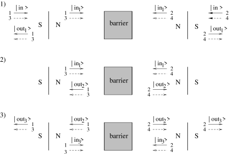
FIG. 4.: Simple illustration of scattering processes. Solid arrows represent electronlike waves, dashed arrows: holelike ones. Numbers enumerate the scattering channels.

Second step: $|in_{1}\rangle$ scatters on the barrier and converts to $|out_{2}\rangle$:

$$|out_{2}\rangle=\hat{S}_{N}|in_{1}\rangle$$ (15)

$$\hat{S}_{N}=\left(\begin{array}[]{cccc}r_{e}&t_{e}&0&0\\ t_{e}&r_{e}^{\prime}&0&0\\ 0&0&r_{h}&t_{h}\\ 0&0&t_{h}&r_{h}^{\prime}\end{array}\right)=\left(\begin{array}[]{cc}s_{0}(E)&\emptyset\\ \emptyset&s_{0}^{*}(-E)\end{array}\right).$$ (22)

Here we used the symmetry $\hat{S}_{N}$ providing $t^{\prime}=t$ and also the time-reversal symmetry of Schrödinger equation, assuring

$$r_{h}(E)=r_{e}^{*}(-E);\;\;\;\;t_{h}(E)=t_{e}^{*}(-E).$$ (23)

Third step: $|out_{2}\rangle$ reaches the $NS$ boundaries from inside. Partially it penetrates into the superconducting electrodes forming the outgoing wave $|out_{3}\rangle$ and partially it is reflected back to the normal region as $|in_{3}\rangle$:

$$|in_{3}\rangle=\hat{S}_{A}|out_{2}\rangle;\;\;\;\;|out_{3}\rangle=\hat{c}_{NS}|out_{2}\rangle,$$ (24)

where the matrices $\hat{S}_{A},\hat{c}_{NS}$ are the Andreev reflection and transmission matrices analogous to $\hat{a}_{s},\hat{c}_{SN}$.

Fourth step: Continue the steps 2 and 3 up to infinity.

The total output can be found from Eqs. (14),(15) and (24) by summing up the geometric series:

$$|out\rangle=|out_{1}\rangle+|out_{3}\rangle+|out_{5}\rangle+\ldots$$ (28)

$$=[\hat{a}_{s}+\hat{c}_{NS}(I-\hat{S}_{N}\hat{S}_{A})^{-1}\hat{S}_{N}\hat{c}_{SN}]|in\rangle\equiv\hat{S}|in\rangle$$

$$\mbox{or}\;\;\;\hat{S}=\hat{a}_{s}+\hat{c}_{NS}(I-\hat{S}_{N}\hat{S}_{A})^{-1}\hat{S}_{N}\hat{c}_{SN}.$$

FIG. 5.: The illustration of the scattering processes. Letters $N,S$ correspond to the normal and superconducting media, the order parameter on both sides is shown. Solid arrows show the electronlike wave propagation, dashed ones show holelike ones. The index $e$ means that the incoming particle is electronlike, subscript $NS$ means that it comes from the normal part ($SN$: from the superconductor; prime indicates that the particle comes from the right. The scattering processes for holes are completely analogous, one has just to replace the index $e$ by $h$ and solid arrows by dashed ones (and vice versa).

The matrix $\hat{S}_{N}$ is given by Eq. (22) and the matrices $\hat{a}_{s},\hat{c}_{SN},\hat{c}_{NS},\hat{S}_{A}$ are constructed from Andreev and normal reflection and transmission amplitudes on $SN$ boundaries which we obtain below.

In their pioneering work Blonder, Tinkham, and Klapwijk [8] considered the following scattering process (see Fig. 5): the electron, propagating from left to right in the normal metal is scattered by the $NS$ boundary. It can be reflected back to the normal medium or transmitted to the superconductor either as an electron or as a hole. We follow their treatment, but use a different normalization of the wave functions to assure unitarity of the scattering matrix. The incoming, reflected and transmitted waves for $NS$ boundary are given by:

$$\psi_{inc}=\frac{1}{\sqrt{q^{+}}}\left(\begin{array}[]{c}1\\ 0\end{array}\right)e^{iq^{+}x},$$ (31)

$$\psi_{refl}=a\frac{1}{\sqrt{q^{-}}}\left(\begin{array}[]{c}0\\ 1\end{array}\right)e^{iq^{-}x}+b\frac{1}{\sqrt{q^{+}}}\left(\begin{array}[]{c}1\\ 0\end{array}\right)e^{-iq^{+}x},$$ (36)

$$\psi_{trans}=c\frac{1}{\sqrt{k^{+}}\sqrt{u_{0}^{2}-v_{0}^{2}}}\left(\begin{array}[]{c}u_{0}\\ v_{0}\end{array}\right)e^{ik^{+}x}$$ (39)

$$+d\frac{1}{\sqrt{k^{-}}\sqrt{u_{0}^{2}-v_{0}^{2}}}\left(\begin{array}[]{c}v_{0}\\ u_{0}\end{array}\right)e^{-ik^{-}x}$$ (42)

where

$$k^{\pm}=\sqrt{2m(\mu\pm\sqrt{E^{2}-\Delta^{2}})}/\hbar.$$ (43)

Our normalization differs from the one used by Blonder, Tinkham, and Klapwijk by prespinor factors $1/\sqrt{q^{\pm}},1/(\sqrt{k^{\pm}}\sqrt{u_{0}^{2}-v_{0}^{2}})$.

The amplitudes $a,b,c,d$ have been found by matching the wave functions and their derivatives on the boundary. We define the scattering amplitudes analogously for the processes on both $NS$ boundaries of the model Josephson junction (Fig. 4) when the phase difference $\varphi$ is maintained between the superconductors, considering electronlike and holelike projectiles coming from the normal medium to the superconductor (corresponding amplitudes are indicated by $NS$ below) and vice versa (index $SN$)—see Fig. 5. In contrast with the work of Blonder,Tinkham, and Klapwijk[8] we do not initially neglect the deviations of projectiles momenta from $k_{F}$.

In terms of these amplitudes the scattering matrices have the following form:

$$\hat{a}_{s}=\left[\begin{array}[]{cccc}b_{e_{SN}}&0&a_{h_{SN}}&0\\ 0&b_{e_{SN}}^{\prime}&0&a_{h_{SN}}^{\prime}\\ a_{e_{SN}}&0&b_{h_{SN}}&0\\ 0&a_{e_{SN}}^{\prime}&0&b_{h_{SN}}^{\prime}\end{array}\right],$$ (48)

$$\hat{S}_{A}=\left[\begin{array}[]{cccc}b_{e_{NS}}^{\prime}&0&a_{h_{NS}}^{\prime}&0\\ 0&b_{e_{NS}}&0&a_{h_{NS}}\\ a_{e_{NS}}^{\prime}&0&b_{h_{NS}}^{\prime}&0\\ 0&a_{e_{NS}}&0&b_{h_{NS}}\end{array}\right],$$ (53)

$$\hat{c}_{SN}=\left[\begin{array}[]{cccc}c_{e_{SN}}&0&d_{h_{SN}}&0\\ 0&c_{e_{SN}}^{\prime}&0&d_{h_{SN}}^{\prime}\\ d_{e_{SN}}&0&c_{h_{SN}}&0\\ 0&d_{e_{SN}}^{\prime}&0&c_{h_{SN}}^{\prime}\end{array}\right],$$ (58)

$$\hat{c}_{NS}=\left[\begin{array}[]{cccc}c_{e_{NS}}^{\prime}&0&d_{h_{NS}}^{\prime}&0\\ 0&c_{e_{NS}}&0&d_{h_{NS}}\\ d_{e_{NS}}^{\prime}&0&c_{h_{NS}}^{\prime}&0\\ 0&d_{e_{NS}}&0&c_{h_{NS}}\end{array}\right].$$ (63)

The scattering amplitudes are again found from the solution of the matching problem on the boundaries. Here we list them in explicit form:

$$a_{e_{SN}}=-2\sqrt{k^{-}k^{+}}(q^{+}+q^{-})u_{0}v_{0}/D,$$ (64)

$$b_{e_{SN}}=-[u_{0}^{2}(q^{+}-k^{+})(q^{-}+k^{-})$$ (65)

$$\;\;\;-v_{0}^{2}(q^{+}-k^{-})(q^{-}+k^{+})]/D,$$ (66)

$$c_{e_{SN}}=2\sqrt{k^{+}q^{+}}(q^{-}+k^{-})u_{0}\sqrt{u_{0}^{2}-v_{0}^{2}}e^{-i\varphi/4}/D,$$ (67)

$$d_{e_{SN}}=2\sqrt{k^{+}q^{-}}(k^{-}-q^{+})v_{0}\sqrt{u_{0}^{2}-v_{0}^{2}}e^{i\varphi/4}/D,$$ (68)

$$a_{e_{NS}}=2\sqrt{q^{-}q^{+}}(k^{+}+k^{-})u_{0}v_{0}e^{-i\varphi/2}/D,$$ (69)

$$b_{e_{NS}}=[u_{0}^{2}(q^{+}-k^{+})(q^{-}+k^{-})$$ (70)

$$\;\;\;-v_{0}^{2}(q^{-}-k^{+})(q^{+}+k^{-})]/D,$$ (71)

$$c_{e_{NS}}=2\sqrt{k^{+}q^{+}}(q^{-}+k^{-})u_{0}\sqrt{u_{0}^{2}-v_{0}^{2}}e^{-i\varphi/4}/D,$$ (72)

$$d_{e_{NS}}=2\sqrt{k^{-}q^{+}}(k^{+}-q^{-})v_{0}\sqrt{u_{0}^{2}-v_{0}^{2}}e^{-i\varphi/4}/D,$$ (73)

where

$$D=u_{0}^{2}(q^{+}+k^{+})(q^{-}+k^{-})-v_{0}^{2}(q^{+}-k^{-})(q^{-}-k^{+}).$$ (74)

Note, that the nonprimed amplitudes correspond to the processes where the projectile comes from the left, so the above values $a_{e_{SN}},b_{e_{SN}}\ldots$ are calculated on the left $SN$ boundary (the phase of the order parameter is equal to $-\varphi/2$), while the amplitudes $a_{e_{NS}},b_{e_{NS}}\ldots$ are on the right boundary (the phase of the order parameter $\varphi/2$).

To obtain the expressions for hole scattering amplitudes (such as $a_{h_{SN}}$) one has to replace in the above formulas $k^{\pm},q^{\pm}$ by $k^{\mp},q^{\mp}$ correspondingly and also to replace $\varphi$ by $-\varphi$. All primed amplitudes are equal to the corresponding nonprimed ones taken at $-\varphi$. Inserting these matrices and $\hat{S}_{n}$ (22) into Eq. (28) we obtain the S-matrix for a general $SCS$ junction.

V Josephson Currents

Knowing the explicit form of the scattering matrix one can find the $\varphi$-dependence of the continuum density of states using Krein’s theorem:

$$\frac{\partial\rho}{\partial\varphi}=\frac{1}{2\pi i}\frac{\partial^{2}}{\partial\varphi\partial E}\ln\det S.$$ (75)

The idea of the proof is given in Appendix A.

Now we have all the required tools to find the Josephson current. The continuum contribution can be expressed in terms of the scattering matrix using Eqs. (5) and (75) [1, 12]:

$$I_{c}=\frac{e}{\pi i\hbar}\int_{\Delta}^{\infty}dE\,\tanh\frac{E}{2k_{B}T}\,\frac{\partial}{\partial\varphi}\ln\det\hat{S}.$$ (76)

This result can be simplified by using the Andreev approximation (that is, neglecting the deviations of $k^{\pm},q^{\pm}$ from $k_{F}$):

$$I_{c}=-\frac{e}{\pi\hbar}\Delta^{2}\sin\varphi\int_{\Delta}^{\infty}$$ (77)

$$\times\frac{E\sqrt{E^{2}-\Delta^{2}}\,\tilde{D}\sin\beta\tanh\frac{E}{2k_{B}T}\,dE}{\{E^{2}-\Delta^{2}\cos^{2}[(\beta-\gamma)/2]\}\{E^{2}-\Delta^{2}\cos^{2}[(\beta+\gamma)/2]\}}$$ (78)

where

$$\ \tilde{D}=|t(E)t(-E)|; \beta=\arg t(E)-\arg t(-E);$$ (79)

$$\tilde{R}=|r(E)r(-E)|; \;\;\;\epsilon=\arg r(E)-\arg r(-E)-\beta;$$ (80)

$$\cos\gamma=\tilde{R}\cos\epsilon+\tilde{D}\cos\varphi$$ (81)

(we follow the definitions of Wendin and Shumeiko[5]).

Equation (78), which is one of the central results of our work, embraces a wide class of Josephson junctions. In particular, Eq. (78) describes arbitrarily long junctions, a problem often avoided. Equation (78) is convenient for qualitative estimations of the continuum contribution to the current. For instance, consider a clean $SNS$ junction. In this case $\beta=EL/(\Delta\xi_{0})$ where $\xi_{0}=\mu/(\Delta k_{F})$ is the superconductor coherence length (for more details see Appendix B). For a short junction ($L\ll\xi_{0}$) $I_{c}$ is small and it is roughly proportional to the junction’s length. In the opposite case of a very long junction ($L\gg\xi_{0}$) the continuum contribution is small again, but for a different reason: the integrand is now a product of the oscillating {$\sin[EL/(\Delta\xi_{0})]$} and decaying ($\approx 1/E^{2}$) functions of energy and the integration over energy results in strong cancellation. However, in some junctions one can expect a significant continuum current: (i)If $\beta,\gamma$ are small (as in the case of some $SIS$ junctions [6]) or, more general, if $\beta\pm\gamma$ is close to $\pi n$ — the denominator in Eq. (78) is small at $E>\Delta$. (ii) If the junction transmission $\tilde{D}$ is large or if it has a sharp maximum at $E>\Delta$ (as in the case of resonant structures like $SINIS$, $SININIS$, etc.) and thus the numerator can also be large.

If the scattering amplitudes of the constriction depend weakly on energy, $\tilde{D},\tilde{R}$ are approximately equal to the transmission and reflection coefficients of the barrier correspondingly and the angles $\beta,\epsilon$ are small. In this case, the integral in Eq. (78) can easily be done at zero temperature:

$$I_{c}\approx-\frac{e\Delta\tilde{D}\sin\varphi}{2\hbar}\frac{\sin\beta}{|\sin[(\beta-\gamma])/2]|+|\sin[(\beta+\gamma)/2]|}.$$ (82)

The spatial separation method can also be used to rederive the known results for the bound state energies and current. The eigenenergies $E_{n}$ correspond to the singular points of energy-dependent scattering matrix. From equation (28) we obtain[1]:

$$\det[I-\hat{S}_{N}(E_{n})\hat{S}_{A}(E_{n})]=0.$$ (83)

Using the definitions of $\hat{S}_{N},\hat{S}_{A}$ [Eqs. (22) and (53)], Andreev approximation, properties (23) of $\hat{S}_{N}$ and the parameters $\tilde{R},\tilde{D},\beta,\epsilon,\gamma$ [Eqs. (79)-(81)] one obtains the following equations for the eigenenergies of the bound states in two equivalent forms:

$$\mbox{Re}\left[\frac{v_{0}^{2}}{u_{0}^{2}}t(E)t^{*}(-E)\right]=\mbox{Re}[r(E)r^{*}(-E)t^{*}(E)t(-E)]$$ (84)

$$+\tilde{D}^{2}\cos\varphi,$$ (85)

$$2\frac{1}{\Delta^{2}}\sqrt{E^{2}\Delta^{2}-E^{4}}\,\sin\beta=\tilde{R}\cos\epsilon+\tilde{D}\cos\varphi.$$ (86)

Equation (86) can be solved with respect to $E$ by squaring and some other algebraic manipulations. The result is

$$E^{2}=\Delta^{2}\cos^{2}\frac{\beta\pm\gamma}{2},\;\mbox{if}\;\sin(\beta\pm\gamma)\geq 0.$$ (87)

The condition $\sin(\beta\pm\gamma)\geq 0$ in (87) is essential, because squaring can produce a redundant solution[13].

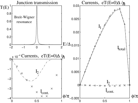
FIG. 6.: Exact numerical calculations for the symmetrical SINIS junction, $\Gamma\approx 0.04\Delta$. Dashed line represents the low-energy state current, dash-dotted shows the edge state current, “+”: the total bound state contribution, “x”: the continuum contribution, solid line: the total Josephson current.

Although the formulas (86) and (87) look like explicit equations for the energy, there might be hidden energy dependence of the scattering amplitudes and consequently of the angles $\beta,\gamma,\epsilon$. Thus equations (86) and (87) are to be solved self-consistently.

Knowing the scattering properties of the barrier one can calculate the $\varphi$-dependent current using Eq. (78) and one of Eqs. (85),(86), and (87). Below we consider several applications of these formulas.

VI $SINIS$ junctions

For the structures containing two $IS$ boundaries (like $SIS,SINIS$ etc.) one can safely use the steplike pair potential approximation,[2, 14] and consequently Eqs. (78),(85),(86), and (87) for quantitative calculations. The $SINIS$ junction is the simplest example of the resonant structure. We solve it analytically using the Breit-Wigner-like formulas for transmission and reflection amplitudes. More precise calculations, taking the exact amplitudes $t,r$ instead of the Breit-Wigner approximation were performed numerically.

Consider the symmetrical $SINIS$ junction. Denote the $N$-part length by $L$ and the single–barrier transmission coefficient by $D$. The Breit–Wigner near-resonance transmission and reflection amplitudes are

$$t=\frac{\Gamma}{E-E_{0}+i\Gamma}e^{i\varphi_{t}};\;\;\;\;r=\frac{E-E_{0}}{E-E_{0}+i\Gamma}e^{i\varphi_{r}}\;,$$ (88)

where $E_{0}$ is the bare resonance level, $\Gamma=\hbar Dv_{F}/L$ and $\varphi_{t},\varphi_{r}$ are some weak (on the scale of $\Gamma$) energy dependent phases which cancel in further calculations.

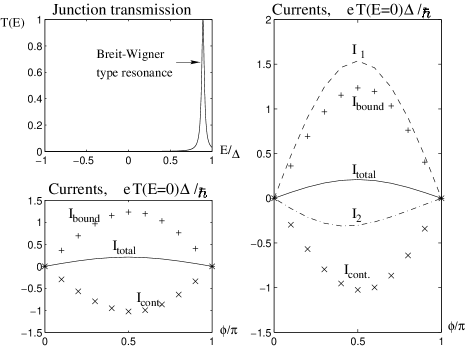
FIG. 7.: Symmetrical SINIS. The resonance width and all line types are the same as at the previous figure, but the resonance itself is not close to the middle of the superconductor gap. The total current is reduced by an order of magnitude compared to the previous case.

Substituting the Breit-Wigner amplitudes from Eq. (88) to Eq. (85) we obtain

$$E^{2}(E_{0}^{2}+\Gamma^{2}+\Delta^{2})+2\Gamma E^{2}\sqrt{\Delta^{2}-E^{2}}$$ (89)

$$=E^{4}+E_{0}^{2}\Delta^{2}+\Delta^{2}\Gamma^{2}\cos^{2}\frac{\varphi}{2}.$$ (90)

This equation has only one positive energy solution and thus it misses the edge states as a result of inadequate accuracy of the Breit-Wigner approximation. Equation (89) is accurate enough only in the neighborhood of the resonance, but not on the scale of $\Delta$. In order to obtain the edge states in Sec. III we have introduced the slow energy dependence of $r_{0}$. Now assume that the resonance is sharp, $\Gamma\ll\Delta$. One can see [for example from the graphic solution of Eq. (89)] that when the bare resonance level lies within the gap, the bound state is close to $|E_{0}|$. In particular, for $E_{0}\ll\Delta$ equation (89) simplifies [5] to

$$E=\sqrt{E_{0}^{2}+\Gamma^{2}\cos\frac{\varphi}{2}}.$$ (91)

From Eq. (91) it follows that the amplitude of the $\varphi$ dependence of such levels is of order of $\Gamma^{2}/E_{0}$ when $E_{0}\gg\Gamma$ and of order of $\Gamma$ for $E_{0}\ll\Gamma$. If the system allows to tune the bare resonance position one can observe the enhancement of the current whenever $E_{0}$ crosses the Fermi level [5, 15]. In the latter case $E=\Gamma\cos\varphi/2$.

In Sec. III we saw that for structures containing a single superconductor there exist bound states on the resonance as well as on pure $IS$ boundary. For $SINIS$ junction one could expect an existence of three bound states: one close to the $|E_{0}|$ and two others close to $\Delta$. Exact numerical calculations not using Breit-Wigner approximation but exact amplitudes $t,r$ for $SINIS$ junction confirm this expectation. The contribution of the “edge” states is, as in the $SIS$ case, proportional to off–resonant transmission, that is to $\Gamma^{2}$. Therefore, these levels can not be found using the Breit-Wigner approximation. Sometimes one of the “interface” levels (or both of them) is pushed to the continuum. As for the continuum contribution, it is proportional to the junction transparency (78) which is of the order of $\Gamma^{2}$.

The numerical solution for the case of a very low lying resonance ($E_{0}\ll\Gamma$) is shown in Fig. 6. It is in a good agreement with the Breit–Wigner model discussed above. However, neither the edge state nor the continuum contribution can be neglected when $E_{0}>\Gamma$. In the example shown in Fig. 7 one edge level is pushed to the continuum (as in the previous case), but the other one contributes and together with the continuum reduces the total current by an order of magnitude. A similar reduction was observed by H.Takayanagi (private communication).

VII $SININIS$ junctions

The $SININIS$ junction represents two coupled normal layers. For a short symmetrical junction without resonances one can find “giant currents” similar to the ones in $SNINS$ [5]. These are the contributions proportional to the square root of the junction transmission rather than to the transmission itself. However, the current-carrying levels are close to each other and thus they are almost equally populated in equilibrium and the “giant” currents strongly compensate each other. This results in a total current which is approximately equal to

$$I_{J}^{standard}=\frac{e\Delta\tilde{D}(E=0)}{\hbar},$$ (92)

a well-known Josephson result. It is interesting to find a structure where the current exceeds this “standard” value.

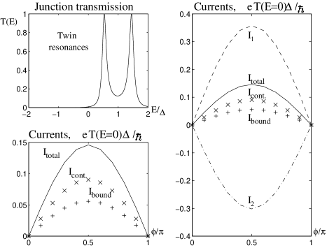
FIG. 8.: The ”twin resonance” structure. The bound and the continuum currents have the same sign.

In this section we present the numerical results for two structures with resonances.

The first one is the short symmetrical $SININIS$ with twin resonances. We have chosen the constriction with one of twin peeks placed within the continuum (Fig. 8). Interesting, that the continuum current exceeds the total bound state current and that both discrete and continuum contributions have the same sign (they often have opposite signs).

The second example (Fig. 9) is the long (about 3 $\xi_{0}$) nonsymmetrical junction. One can see again the strong compensation of individual levels, but the total current exceeds the standard value $e\Delta\tilde{D}(0)/\hbar$ by about a factor of 2. More important, the individual level currents exceed the $I_{J}^{standard}$ hundreds of times and the levels, supporting these currents are split significantly ($E_{1}\approx 0.75\Delta,E_{2}\approx 0.89\Delta,E_{3}\approx 0.95\Delta$). Thus it may be possible to populate the bound states nonuniformly (for example by resonant electromagnetic pumping or by coupling to the additional electrode [6]) and to enhance the Josephson current by order(s) of magnitude.

FIG. 9.: Currents in a long ($\approx 3\xi_{0}$) nonsymmetrical $SININIS$ junction. In this case there are three bound states and, correspondingly three bound currents ($I1,\;I2,\;I3$). Although each one of them exceeds the “standard” value for Josephson current many times, the total current is just two times greater than that.

VIII Conclusions

In the present work the dc Josephson effect was investigated and explicit formulas for Josephson current were obtained in 1D case. We used the approach suggested by I.O.Kulik [4] based on the solution of Bogolubov - de Gennes equations. This technique treats the contributions of discrete and continuum energy states separately. Unlike the usual way [4, 6, 16], we have not used the Landauer-type consideration to find the continuum current, but Beenakker’s approach allowing to derive both discrete and continuum contributions from the most general thermodynamic relations. We have also specified the Beenakker’s idea of spatial separation of the superconductors from the barrier for 1D case and developed it for infinitesimally thin separating layers (they do not have to be long compared to the Fermi wavelength $\lambda_{F}$). Such insertion of fictitious normal layers should be treated as a mathematical trick only, reducing quite complicated Josephson problem to Andreev reflection [8, 17] and relatively simple scattering problem of normal electrons on the barrier.

Our results are applicable to a wide class of 1D elements. The only approximations we used are: (i)Andreev approximation, $\Delta\ll\mu$. (ii) Existence of a large barrier on the boundary of the superconductor. (iii) Low current, $\hbar e\rho_{s}/(mJ_{Q})$ (where $J_{Q}$ is the current density and $\rho_{s}$ is the superconducting density) to be much greater than all characteristic lengths such as coherence length, junction width, etc. The last two conditions are required to justify the steplike pair potential approximation (3).

Applying our formulas to different junctions we have appreciated the crucial role of the continuum contribution even in cases where this was not expected. The continuum current is often neglected in short (compared to the coherence length) junctions [4, 5], but in some short structures we found that the continuum current can be of order of the bound-state current or even exceed it. We have found also an unusual enhancement (rather than decrease) of the total current by the continuum contribution.

It was found in the paper by Wendin and Shumeiko that total Josephson current might result from almost complete cancellation of huge bound state currents flowing in the opposite directions. The states supporting these giant currents lie very close to each other, so it is hard to populate them differently and the giant currents are almost canceled. We found some structures which we believe can be built experimentally, where the level separation is of order of $\Delta$ and the individual currents supported by these states exceed the usual Josephson value $e\Delta\tilde{D}(E=0)/\hbar$ tens or hundreds of times. We still could not avoid the strong cancellation of individual currents and the equilibrium current is of order of its standard value (see above), and in our best structures it is enhanced by a factor of 2-3. We expect that the current in such junctions can be much enhanced by appropriate population of individual bound states (for example, by microwave pumping or by coupling to another electrode). However, just a large energy separation of Andreev states does not guarantee the lack of cancellation of their contributions.

We benefited from stimulating discussions with B. Laikhtman and V. Shumeiko. We also thank E. Balkovsky for his kind help. This work was supported by the Israel Academy of Science and by the German-Israeli Foundation (GIF).

A Krein’s theorem

In this appendix we find the relationship between the continuum density of states to the scattering matrix. We use the definition of the density of states for the continuum

$$\rho=-\frac{1}{\pi}\mbox{Im Tr}\,G$$ (A1)

where $G$ is the retarded Green’s function $G=(E-H+i\epsilon)^{-1}$, $H$ is considered to be a full Hamiltonian of the system, including the scatterer contribution: $H=H_{0}+V$, and $H_{0}$ is an unperturbed one. In terms of these variables the scattering operator takes the form

$$S=\Omega^{-\dagger}\Omega^{+}\equiv G_{0}^{-1}GGG_{0}^{-1}.$$ (A2)

Here $\Omega^{\pm}=[E-H\pm i\epsilon]^{-1}[E-H_{0}\pm i\epsilon]$ is the Möller wave operator. Krein’s theorem [7] claims that for any two linear operators $H_{1},H_{2}$ (for example for the free Particle Hamiltonian and the perturbed Hamiltonian) holds:

$$Tr[(H_{1}-EI)^{-1}-(H_{2}-EI)^{-1}]$$ (A4)

$$=-\frac{\partial}{\partial E}\ln\det[(H_{1}-EI)(H_{2}-EI)^{-1}].$$

The idea of the proof is simple: in the basis of eigenfunctions the operator takes the diagonal form, so

$$\frac{\partial}{\partial E}\ln\det(H_{1}-EI)$$ (A10)

$$=\frac{\partial}{\partial E}\ln\det\left(\begin{array}[]{ccc}E_{1}-E&0&\ldots\\ 0&E_{2}-E&\\ \vdots&&\ddots\end{array}\right)$$

$$=-\sum_{n}\frac{1}{E_{n}-E}=-\mbox{Tr}(H_{1}-EI)^{-1}.$$

The theorem stated follows from Eq. (A10) and the analogous relation for $H_{2}$. Note that it is not required to diagonalize both Hamiltonians simultaneously. From the definitions of the DOS (A1) and the definition of the scattering matrix (A2) one obtains

$$\rho-\rho_{0}=\frac{1}{2\pi i}\frac{\partial}{\partial E}\ln\det S\;,$$ (A11)

where $\rho_{0}$ is the free particle DOS and $\rho$ is the DOS of the scattering problem. We also used the unitarity of the scattering matrix.

The theorem is valid in both the normal and the superconducting cases, in the latter case one has to treat the corresponding Hamiltonians as BCS or Bogolubov Hamiltonians and to use the superconductor - to - superconductor scattering matrix. Noting that $\rho_{0}$ is $\varphi$ independent (up to small mesoscopic corrections) one can calculate the continuum contribution to the current using Eqs. (5) and (A11).

B Applications of the Spatial Separation Method

1 Andreev reflection

In this appendix we rederive the formulas for Andreev reflection from $NS$ boundary with a barrier using the spatial separation method. Consider the reflection of a quasiparticle from a point “impurity” modeled by a $\delta$-function barrier, separated by a distance $l$ from an ideal $NS$ boundary. More precisely, we use the Bogolubov-de Gennes [14] Hamiltonian with $V(x)=+V_{0}\delta(x)$ and $\Delta(x)=\Delta_{0}\theta(x+l)$ where $\theta$ is the Heaviside step function. Taking into account multiple reflections from the barrier and $Andreev$ reflections from ideal (barrier free) $NS$ boundary [8, 17] we obtain for incoming electron-like particle

$$a=\frac{t_{e}t_{h}a_{e}e^{i(q^{+}-q^{-})l}}{1-r^{\prime}_{e}r^{\prime}_{h}a_{e}a_{h}e^{2i(q^{+}-q^{-})l}}$$ (B1)

$$b=r_{e}+\frac{r^{\prime}_{h}t_{e}^{2}a_{e}a_{h}e^{2i(q^{+}-q^{-})l}}{1-r^{\prime}_{e}r^{\prime}_{h}a_{e}a_{h}e^{2i(q^{+}-q^{-})l}}$$ (B2)

where $a,b$ are the total Andreev and normal reflection amplitudes, $r_{e},t_{e},r_{h},t_{h}$ are the barrier reflection and transmission amplitudes for electron and hole, $a_{e},a_{h}$ are analogous Andreev reflection amplitudes, prime corresponds to the left-going particle. Restricting our consideration to energies of order of $\Delta_{0}$ and neglecting all $\Delta_{0}/\mu$ terms (Andreev approximation) we have

$$a_{e}=a_{h}=\frac{v_{0}}{u_{0}}\,,\;\;\;\;r_{e}=r^{\prime}_{e}=\frac{-iZ}{1+iZ}\,,\;\;\;\;t_{e}=t^{\prime}_{e}=\frac{1}{1+iZ}\,,$$ (B3)

where $Z=2mV_{0}/(\hbar^{2}k_{F})$. Corresponding normal reflection and transmission amplitudes for holes are just the complex conjugated ones for electrons. Substituting these quantities to Eq. (B2) we obtain

$$a=\frac{u_{0}v_{0}e^{i(q^{+}-q^{-})l}}{u_{0}^{2}+(u_{0}^{2}-v_{0}e^{2i(q^{+}-q^{-})l})Z^{2}}\,,$$ (B4)

$$b=-\frac{(u_{0}^{2}-v_{0}e^{2i(q^{+}-q^{-})l})(iZ+Z^{2})}{u_{0}^{2}+(u_{0}^{2}-v_{0}e^{2i(q^{+}-q^{-})l})Z^{2}}.$$ (B5)

This intuitively clear two-step method allows to get the final result more easily than by a direct solution of the matching problem ($8\times 8$ linear system). Its advantage becomes even more pronounced in more complicated problems with larger number of boundaries. In the limit $l\rightarrow 0$ our results tend to the ones obtained by Blonder, Tinkham, and Klapwijk [8] for reflection from $NS$ boundary with a barrier [18].

2 $SNS$ junction.

As an illustration of the previous results, consider the well-investigated example of $SNS$ contact (here $N$ indicates a normal metal, $S$ a superconductor).

The $SNS$ constriction includes no barrier, it consists of a piece of a clean normal metal of length $L$ sandwiched between the superconductors. For this structure

$$r(E)=0;\;\;t(E)=e^{iq^{+}L};\;\;t^{*}(-E)=e^{-iq^{-}L};\;\;\tilde{D}=1.$$ (B6)

Substituting these expressions to Eq. (85) and using the relation $v_{0}/u_{0}=e^{-i\arccos E/\Delta}$ we obtain the Kulik’s result for bound states [4]:

$$2\arccos\frac{E_{n}}{\Delta}-(q_{n}^{+}-q_{n}^{-})L\pm\varphi=2\pi n.$$ (B7)

The momenta $q^{+},q^{-}$ are very close to $k_{F}$. Expanding $q^{+},q^{-}$ as a function of energy around $k_{F}$ we obtain

$$q^{\pm}\approx k_{F}\pm\frac{E}{2\Delta\xi_{0}}$$ (B8)

where $\xi_{0}=\mu/(\Delta)(1/k_{F})$ is the superconductor coherence length. Using Eqs. (78), (B6), and (B8) one can find the continuum contribution:

$$I_{c}=-\frac{e}{\pi\hbar}\Delta^{2}\sin\varphi\int_{\Delta}^{\infty}$$ (B9)

$$\times\frac{E\sqrt{E^{2}-\Delta^{2}}\,\sin{(EL/\Delta\xi_{0})}\tanh{(E/2k_{B}T)}\,dE}{(E^{2}-\Delta^{2}\cos^{2}\{[(EL/\Delta\xi_{0})-\varphi]/2\})(E^{2}-\Delta^{2}\cos^{2}\{[(EL/\Delta\xi_{0})+\varphi]/2\})}.$$ (B10)

An analogous equation was obtained by Bagwell [16]. Relations (B7) and (B9) should not be treated too seriously in quantitative aspect. The problem is that the step-like pair potential hypothesis fails; conversely, $\Delta$ changes on scale $\xi_{0}$ [14].

^∗Present address: University of Alberta, Edmonton, AB, Canada T6G 2J1.

REFERENCES

- [1] C. W. J. Beenakker Transport Phenomena in Mesoscopic Physics (Springer-Verlag, Berlin, 1992).
- [2] K. K. Likharev, Rev. Mod. Phys. 51, 101 (1979).
- [3] M. Yu. Kupriyanov and V. Lukichev, Fiz. Nizk. Temp. 8, 1045 (1982) [Sov. J. Low Temp. Phys. 8, 526 (1982)].
- [4] I. O. Kulik and A. N. Omel’yanchuk, Zh. Eksp. Teor. Fiz. 57, 1745 (1969) [Sov. Phys. JETP 30, 944 (1970)].
- [5] G. Wendin and V. Shumeiko, Superlattices and Microstruct. 20, 569 (1996).
- [6] G. Wendin and V. Shumeiko, Phys. Rev. B 53, R6006 (1996).
- [7] M. G. Kreĭn, Sov. Math. Dokl. 3 1071 (1962).
- [8] G. E. Blonder, M. Tinkham, and T. M. Klapwijk, Phys. Rev. B 25, 4515 (1982).
- [9] V. Ambegaokar and A. Baratoff, Phys. Rev. Lett. 10 468 (1963); A. A. Zubkov and M. Yu. Kupriyanov, Fiz. Nizk. Temp. 9, 548 (1983) [Sov. J. Low Temp. Phys. 9, 279 (1983)].
- [10] B. Laikhtman (private communication).
- [11] L. D. Landau and E. M. Lifshitz, Quantum Mechanics (Pergamon, New York , 1975).
- [12] E. Akkermans, A. Auerbach, J. E. Avron and B. Shapiro, Phys. Rev. Lett. 66, 76 (1991).
- [13] We are especially grateful to Vitaly Shumeiko for clarifying this point.
- [14] P. G. deGennes Superconductivity of metals and alloys. (Addison-Wesley, New York, 1989).
- [15] H. Takayanagi and T. Akazaki, Jpn. J. Appl. Phys., Part 1 34, 6977 (1995).
- [16] P. F. Bagwell, Phys. Rev. B 46, 12573 (1994).
- [17] A. F. Andreev, Zh. Eksp. Teor. Fiz. 46, 1823 (1964) [Sov. Phys. JETP 19, 1228 (1964)].
- [18] The transmission amplitudes would differ from the BTK values by factor of due to different normalization of the wave functions. The amplitudes are the same with either normalization (under Andreev approximation).