Adsorption of a random heteropolymer at a potential well revisited: location of transition point and design of sequences

Abstract

The adsorption of an ideal heteropolymer loop at a potential point well is investigated within the frameworks of a standard random matrix theory. On the basis of semi–analytical/semi–numerical approach the histogram of transition points for the ensemble of quenched heteropolymer structures with bimodal symmetric distribution of types of chain’s links is constructed. It is shown that the sequences having the transition points in the tail of the histogram display the correlations between nearest–neighbor monomers.

I Introduction

The problem of adsorption of an ideal heteropolymer chain with random quenched chemical structure (i.e. sequence of links) is far from being new and is well represented in the literature.

The simple diffusive approach [1, 2, 3, 4] provides us complete understanding of the homopolymer and block–copolymers adsorption in various geometries. More advanced renormalization group methods [5, 6] and power series analysis [7] applied to random chains with a disordered sequence of links delivers an important information about the thermodynamic properties of ideal polymers near the transition point from delocalized (Gaussian) to localized (adsorbed) regimes. A mathematical formalism based on perturbation theory gives reasonable results for a phase transition in solid–on–solid (SOS) models with quenched impurities [8]. Many conclusions of [8] correlate with those obtained by RG analysis in [6]. Problems dealing with localization of disordered polymers at selective interfaces [9, 10, 11] should be also mentioned in the context of discussed problems.

However even since early 80s during almost 20 years of intent attention some important questions of heteropolymer adsorption remain still open. One of them, the most intriguing, to our point of view, concerns the location of a point of a phase transition from coil to localized (adsorbed at a potential well) state.

In this paper we consider the model of an ideal, i.e. self–intersecting ring polymer chain consisting of two types of links, ”black” and ”white” organized in different chemical structures having different energies in the single point–like potential well. We distinguish between the following models of chemical structures:

1. ”Canonically quenched” sequence—positions of ”black” and ”white” links are uniquely fixed for a given chain structure and cannot exchange in course of chain fluctuations; the chemical structure is prepared from ”black” and ”white” links at random with prescribed probabilities.

2. ”Microcanonically quenched” sequence—positions of ”black” and ”white” links are again uniquely fixed for a given chain structure and satisfy an extra constraint: the total number of ”black” and ”white” links per chain is conserved for all realizations of chain structures.

Our consideration is semi-analytical/semi-numerical. Namely, the closure of an ideal $N$–link chain in a ring enables us to integrate from the very beginning over all space degrees of freedom for quenched sequences of links and explicitly rewrite the Green’s function of a chain as a quotient of determinants of two $N\times N$–matrices with random coefficients on the main diagonals. The transition point corresponds to the situation when the denominator of the quotient becomes zero. This last question for large $N$ and different models of chemical structures is analyzed numerically.

The results are exposed in a form of histograms showing how many sequences have the transition points at a given energy. Choosing the sequences which have the transition points in the tail of the histogram we found that these sequences have effective correlations between nearest–neighbor monomers for the model (2) and do not exhibit any correlations for the model (1).

II The model

Consider an $N$–link ideal (i.e. self–intersecting) Gaussian polymer chain in $d$–dimensional space. Suppose that the chain forms a ring and attach the first and the last chain’s segments to the origin. All segments are painted in ”black” or ”white” colors, designating different interaction energies with the potential well located at the origin. There is no interaction of chain’s links between themselves or between a link and any point in $d$–dimensional space distinct from the origin. Increasing the interaction energy, we could provoke the transition from extended (coil) to localized (adsorbed) state of the macromolecule. The transition is governed by the interplay between entropic forces tending to expel the chain and contact potential interactions which gain the energy in a compact polymer configuration.

The said above can be easily rewritten in a formal way. Let us introduce the joint distribution function $G_{N}({\bf x}_{1},{\bf x}_{2},...,{\bf x}_{N})$ having sense of a probability that the links with numbers $1,2,...,N$ of the $N$–step chain are located at the points ${\bf x}_{1},{\bf x}_{2},...,{\bf x}_{N}$ in $d$–dimensional space. The Markov structure of our polymer chain ensures the presence of correlation only between the neighboring segments of length $a$ and allows us to set

$$P_{N}({\bf x}_{1},{\bf x}_{2},...,{\bf x}_{N})=g({\bf x}_{1},{\bf x}_{2})g({\bf x}_{2},{\bf x}_{3})...g({\bf x}_{N-1},{\bf x}_{N})$$

where the transition probability $g({\bf x}_{1},{\bf x}_{2})$ satisfies the normalization condition $\int g({\bf x},{\bf x}^{\prime})d{\bf x}=1$ and for simplicity is supposed to be Gaussian:

$$g({\bf x})=\left(\frac{d}{2\pi a^{2}}\right)^{d/2}e^{-\frac{d|{\bf x}|^{2}}{2a^{2}}}$$ (1)

The Green’s function $G({\bf x}_{N},N)\equiv\int G_{N}({\bf x}_{1},{\bf x}_{2},...,{\bf x}_{N})d{\bf x}_{1}d{\bf x}_{2}...d{\bf x}_{N-1}$ is defined as follows

$$G({\bf x}_{N},N)=\int\prod_{i=1}^{N}\left[g({\bf x}_{i-1},{\bf x}_{i})e^{-\phi({\bf x}_{i})/T}\right]d^{d}x_{1}...d^{d}x_{N-1}.$$ (2)

where $e^{-\phi({\bf x}_{i})/T}$ is the Boltzmann weight of $i^{\rm th}$ chain segment in the potential well at the origin (compare to [6]):

$$e^{-\phi({\bf x}_{i})/T}=1+\beta_{i}\delta({\bf x}_{i});\quad\beta_{i}=\left\{\begin{array}[]{ll}e^{-u_{\rm b}}-1&$\mbox{if the segment $i$ is "black"}$\\ e^{-u_{\rm w}}-1&$\mbox{if the segment $i$ is "white"}$\end{array}\right.$$ (3)

and $u_{\rm b,w}$ is the dimensionless energy (everywhere below we set $T=1$).

Now we can write the recursion equation for the Green’s function (2), expressing $G({\bf x}_{i+1},{i+1})$ in terms of $G({\bf x}_{i},i)$ and corresponding Boltzman weights for $0\leq i\leq N$. Performing Fourier transform and taking into account (3) we arrive at the following integral equation in the momentum space

$$G({\bf k},i+1)=g({\bf k})G({\bf k},i)+(2\pi)^{-d}\beta_{i+1}\int g({\bf k}^{\prime})G({\bf k}^{\prime},i)d^{d}k^{\prime}$$ (4)

where

$$g({\bf k})=e^{-|{\bf k}|^{2}a^{2}/2d}$$ (5)

In order to make the system of equations (4) closed and nonuniform we should take into account the initial and boundary conditions. Let us point out that for open chains the precise form of initial and boundary conditions does not affect in the thermodynamic limit the phase transition point (see, for example, [12]). The same we expect also for closed chains. Suppose that the last segment (with $i=N$) is linked to the origin by some sufficiently weak dimensionless potential $f$. Without the loss of generality we may chose $f$ in the simplest form: $f({\bf k})\equiv f={\rm const}$. The presence of the potential $f$ increases the probability $\tilde{G}(k,N)$ to find the $N$’s chain link near the origin. If $|f|\ll 1$ we may set in the linear approximation:

$$\tilde{G}({\bf k},i=N)=G({\bf k},i=N)+f$$ (6)

Using the fact that the chain is closed, we complete equations (4) by the following one:

$$G({\bf k},i=1)=g({\bf k})\tilde{G}({\bf k},i=N)+(2\pi)^{-d}\beta_{1}\int g({\bf k}^{\prime})\tilde{G}({\bf k},i=N)d^{d}k^{\prime}$$ (7)

(as we shall see later $f$ does not enter the final expression for the transition point).

The system of $N$ equations (4)–(7) is closed. This enables us to write it as a single matrix–integral equation for the $N$–component ”spinor” Green’s function ${\bf G}({\bf k})=\{G({\bf k},1),G({\bf k},2),...,G({\bf k},N-1),G({\bf k},N)\}$. Hence we get:

$${\bf G}({\bf k})=\hat{M}g({\bf k}){\bf G}({\bf k})+(2\pi)^{-d}\hat{\beta}\hat{M}\int g({\bf k}^{\prime}){\bf G}({\bf k}^{\prime})d^{d}k^{\prime}+{\bf F}({\bf k})$$ (8)

with

$$\hat{M}=\left(\begin{array}[]{ccccc}0&0&0&\dots&1\\ 1&0&0&\dots&0\\ 0&1&0&\dots&0\\ 0&0&1&\dots&0\\ \vdots&\vdots&\vdots&&\vdots\end{array}\right),\quad\hat{\beta}=\left(\begin{array}[]{cccccc}\beta_{1}&0&0&\dots&0\\ 0&\beta_{2}&0&\dots&0\\ 0&0&\beta_{3}&\dots&0\\ \vdots&\vdots&\vdots&\ddots&\vdots\\ 0&0&0&\dots&\beta_{N}\end{array}\right),$$ (9)

and

$${\bf F}({\bf k})=\Big{(}\left(g({\bf k})+(d/2\pi a^{2})^{\frac{d}{2}}\right)f,0,\dots,0\Big{)}^{T}$$ (10)

Let us rearrange the terms in (8) as follows

$${\bf G}({\bf k})=\left(\hat{I}-g({\bf k})\hat{M}\right)^{-1}\Big{[}(2\pi)^{-d}\hat{\beta}\hat{M}\int g({\bf k}^{\prime}){\bf G}({\bf k}^{\prime})d^{d}k^{\prime}+{\bf F}({\bf k})\Big{]}$$ (11)

where $\hat{I}$ is $N\times N$ identity matrix. Integrating l.h.s and r.h.s of (11) with the weight $g({\bf k})$ over all ${\bf k}$, we arrive at the algebraic matrix equation for the function ${\bf A}=\{A_{1},A_{2},...,A_{N}\}$, where $A_{i}=\int g({\bf k})G({\bf k},i)d^{d}k$:

$${\bf A}=(2\pi)^{-d}\left[\int g({\bf k})\left(\hat{I}-g({\bf k})\hat{M}\right)^{-1}\hat{\beta}\hat{M}\;d^{d}k\right]{\bf A}+{\bf F}$$ (12)

The straightforward computations show that the $N\times N$ matrix $\hat{C}=\left(\hat{I}-g({\bf k})\hat{M}\right)^{-1}\hat{\beta}\hat{M}$ has the form:

$$\hat{C}=\left(\begin{array}[]{lllll}\beta_{2}c_{1}&\beta_{3}c_{2}&\beta_{4}c_{3}&\dots&\beta_{1}c_{N}\\ \beta_{2}c_{N}&\beta_{3}c_{1}&\beta_{4}c_{2}&\dots&\beta_{1}c_{N-1}\\ \beta_{2}c_{N-1}&\beta_{3}c_{N}&\beta_{4}c_{1}&\dots&\beta_{1}c_{N-2}\\ \vdots&\vdots&\vdots&\ddots&\vdots\\ \beta_{2}c_{2}&\beta_{3}c_{3}&\beta_{4}c_{4}&\dots&\beta_{1}c_{1}\end{array}\right)$$ (13)

with the coefficients

$$c_{i}\equiv c_{i}({\bf k})=-\frac{g^{N-i}({\bf k})}{g^{N}({\bf k})-1},\quad i\in[1,N]$$ (14)

and the vector ${\bf F}=(F_{1},F_{2},\dots,F_{N})^{T}$ has components

$$F_{i}=\frac{f}{(2\pi)^{d}}\int\left(g({\bf k})+(d/2\pi a^{2})^{\frac{d}{2}}\right)c_{N-i+1}({\bf k})d^{d}k$$ (15)

Hence the vector ${\bf A}$ obeys the system of equations

$$\left\{\begin{array}[]{llllllllllllll}A_{1}&=&\beta_{2}a_{1}A_{1}&+&\beta_{3}a_{2}A_{2}&+&...&+&\beta_{N}a_{N-1}A_{N-1}&+&\beta_{1}a_{N}A_{N}&+&F_{1}\\ A_{2}&=&\beta_{2}a_{N}A_{1}&+&\beta_{3}a_{1}A_{2}&+&...&+&\beta_{N}a_{N-2}A_{N-1}&+&\beta_{1}a_{N-1}A_{N}&+&F_{2}\\ A_{3}&=&\beta_{2}a_{N-1}A_{1}&+&\beta_{3}a_{N}A_{2}&+&...&+&\beta_{N}a_{N-3}A_{N-1}&+&\beta_{1}a_{N-2}A_{N}&+&F_{3}\\ ...&&&&&&&&&\\ A_{N-1}&=&\beta_{2}a_{3}A_{1}&+&\beta_{3}a_{4}A_{2}&+&...&+&\beta_{N}a_{1}A_{N-1}&+&\beta_{1}a_{2}A_{N}&+&F_{N-1}\\ A_{N}&=&\beta_{2}a_{2}A_{1}&+&\beta_{3}a_{3}A_{2}&+&...&+&\beta_{N}a_{N}A_{N-1}&+&\beta_{1}a_{1}A_{N}&+&F_{N}\end{array}\right.$$ (16)

where the coefficients $a_{i}$ for $1\leq i\leq N$ are defined as follows

$$a_{i}=(2\pi)^{-d}\int g({\bf k})c_{i}({\bf k})d^{d}k=\left(\frac{d}{2\pi a^{2}N}\right)^{d/2}\zeta\left(\frac{d}{2},\frac{N+1-i}{N}\right);$$ (17)

Solving the corresponding system of linear equations via the standard Kramers method, we arrive at the following expression for the values $\beta_{i+1}A_{i}$:

$$\beta_{i+1}A_{i}=\frac{{\rm det}\hat{A}^{\prime}(i)}{{\rm det}\hat{A}},\quad i\in[1,N];\quad\mbox{(by definition $\beta_{N+1}=\beta_{1}$)}$$ (18)

where the $N\times N$ matrix $\hat{A}$ reads

$$\hat{A}=\left(\begin{array}[]{llllll}a_{1}-\beta_{2}^{-1}&a_{2}&a_{3}&\dots&a_{N-1}&a_{N}\\ a_{N}&a_{1}-\beta_{3}^{-1}&a_{2}&\dots&a_{N-2}&a_{N-1}\\ a_{N-1}&a_{N}&a_{1}-\beta_{4}^{-1}&\dots&a_{N-3}&a_{N-2}\\ \vdots&\vdots&\vdots&\ddots&\vdots&\vdots\\ a_{3}&a_{4}&a_{5}&\dots&a_{1}-\beta_{N}^{-1}&a_{2}\\ a_{2}&a_{3}&a_{4}&\dots&a_{N}&a_{1}-\beta_{1}^{-1}\end{array}\right)$$ (19)

and the $N\times N$ matrix $\hat{A}^{\prime}(i)$ is obtained from the matrix $\hat{A}$ by replacing the $i^{\rm th}$ column by the vector $-{\bf F}$.

Equations (18)–(19) enable us to rewrite $N$ linearly independent components of the ”spinor” ${\bf G}({\bf k})=\{G_{1}({\bf k}),G_{2}({\bf k}),...,G_{N}({\bf k})\}$ (see (11)) in a compact form

$$G_{i}({\bf k})=(2\pi)^{-d}\Big{[}{\rm det}\hat{A}\Big{]}^{-1}\sum_{j=1}^{N}c_{j-i+1}({\bf k})\,{\rm det}\hat{A}^{\prime}(j)+(\hat{I}-g({\bf k})\hat{M})^{-1}{\bf F}({\bf k})$$ (20)

where $c_{j-i+1}({\bf k})=c_{N-(j-i+1)}({\bf k})$ if $j-i+1\leq 0$.

The transition point from delocalized (coil) to the adsorbed (globule) state of a heteropolymer ring is manifested in the divergence of the Green’s function $G_{i}({\bf k})$ (20) for any $i\in[1,N]$. Thus the transition point is determined by the equation

$${\rm det}\hat{A}=0$$ (21)

where the matrix $\hat{A}$ is given by (19). Let us pay attention to the fact that equation (21) is very general: it is valid for any type of disorder and number of species (i.e. sorts of the links).

For any finite chain lengths we can define only a transition region which due to the supposed self–averaging becomes sharper and sharper as the chain length increases, tending to a single point in the thermodynamic limit $N\to\infty$.

Before passing to numerical solution of (21) for different randomly generated sequences belonging to canonically– and microcanonically quenched chemical structures, let us derive analytically the transition point for the effective homopolymer ring chain. In this case one can preaverage the partition function of the chain over the distribution of ”black” and ”white” links. Let us take $u_{\rm b}=u,\;u_{\rm w}=-u$ and suppose that the number of ”black” links is equal to the number of ”white” ones. Then

$$\beta_{i}\equiv\beta_{\rm av}=\frac{e^{-u}+e^{u}}{2}-1=\cosh u-1$$ (22)

for all $1\leq i\leq N$.

Remind that for $N$–link open homopolymer chain attached by one end at the origin in a potential well, the critical value $\beta_{\rm open}$ of a transition point in $d$–dimensional space in the limit $N\to\infty$ reads [6, 4]

$$\beta_{\rm open}^{-1}=\left(\frac{d}{2\pi a^{2}}\right)^{d/2}\left.\zeta\left(\frac{d}{2}\right)\right|_{{d=3}\atop{a=1}}\approx 0.86188$$ (23)

The transition point of a closed chain can be analytically evaluated in the effective homopolymer case (22). If all $\beta_{i}$ are equal, then the matrix $\hat{A}$ (see eq.(12)) is so–called circulant and its eigenvalues are [13]

$$\lambda_{m}=\sum_{j=1}^{N}a_{j}e^{i2\pi m(j-1)/N},\quad m\in[0,N-1]$$ (24)

Eq. (21) is true when $\beta^{-1}$ equals to one of the eigenvalues $\lambda_{m}$ that must be real. Thus

$$\begin{array}[]{lll}\beta^{-1}_{\rm av}&=&\displaystyle\sum_{j=1}^{N}a_{j}=\left(\frac{d}{2\pi a^{2}N}\right)^{d/2}\sum_{i=1}^{N}\sum_{k=0}^{\infty}\frac{1}{(k+1+(1-i)/N)^{d/2}}\\ &=&\displaystyle\left(\frac{d}{2\pi a^{2}}\right)^{d/2}\sum_{i=0}^{N-1}\sum_{k=1}^{\infty}\frac{1}{(Nk-i)^{d/2}}=\left(\frac{d}{2\pi a^{2}}\right)^{d/2}\sum_{j=1}^{\infty}\frac{1}{j^{d/2}}\\ &=&\displaystyle\left(\frac{d}{2\pi a^{2}}\right)^{d/2}\zeta\left(\frac{d}{2}\right)=\beta_{\rm open}^{-1}\end{array}$$ (25)

Hence, in 3D–space for $a=1$ we have

$$u_{\rm tr}^{\rm av}={\rm arccosh}[\beta_{\rm av}+1]={\rm arccosh}\left[\left(\frac{3}{2\pi}\right)^{3/2}\zeta\left(\frac{3}{2}\right)+1\right]\approx 1.405$$

Let us pay attention to the fact that the adsorption points of ring and open chains coincide in the thermodynamic limit. This is consistent with the statement on independence of the point of 2nd order phase transition on the boundary conditions [14]. Moreover, the interesting feature of (25) consists in the fact that the value $\beta_{\rm av}$ does not depend on $N$ for ring chains.

III Numerical results for quenched sequences of links.

In this section we solve numerically Eq.(21) for two different types of bimodal distribution of links with $u_{\rm b}=u,\;u_{\rm w}=-u$: (1) canonically quenched and (2) microcanonically quenched. Recall that in case (1) ”white” and ”black” links appear in the sequence independently with equal probability $\frac{1}{2}$; while in case (2) the total number of ”black” and ”white” links per chain is exactly $\frac{N}{2}$. We have generated ensembles of $10\;000$ chains of $N$ segments each for both of models (1) and (2). The distribution of transition points $W(u)$ in cases (a) and (b) is depicted in fig.1 for $N=100$.

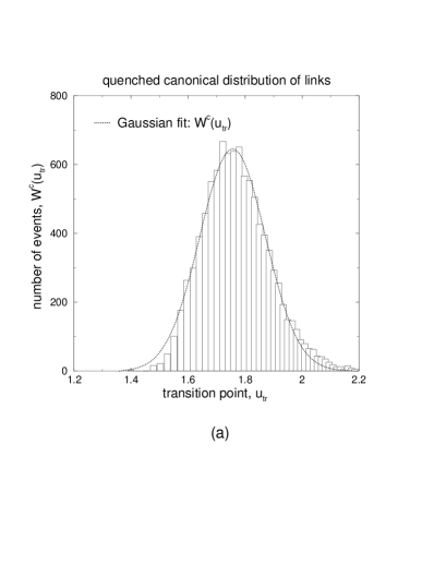
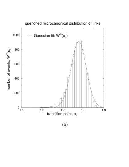
FIG. 1.: Distribution of transition points for (a) canonical and (b) microcanonical sequences of links.

The shape of histograms in fig.1a,b are correspondingly fitted by Gaussian curves

$$W^{\rm c}(u_{\rm tr})=A^{\rm c}e^{-\frac{(u_{\rm tr}-\left<u^{\rm c}_{\rm tr}\right>)^{2}}{2(\sigma^{\rm c})^{2}}};\quad W^{\rm m}(u_{\rm tr})=A^{\rm m}e^{-\frac{(u_{\rm tr}-\left<u^{\rm m}_{\rm tr}\right>)^{2}}{2(\sigma_{\rm m})^{2}}};$$

For $N=100$ the parameters $A^{\rm c,m},\,\left<u^{\rm c,m}_{\rm tr}\right>,\,\sigma_{\rm c,m}$ are as follows:

$$\left\{\begin{array}[]{l}A^{\rm c}=644.78\\ \left<u^{\rm c}_{\rm tr}\right>=1.756\\ \sigma_{\rm c}=0.116\end{array}\right.\qquad\left\{\begin{array}[]{l}A^{\rm m}=908.49\\ \left<u^{\rm m}_{\rm tr}\right>=1.778\\ \sigma_{\rm m}=0.039\end{array}\right.$$

To predict the numerical values of $\left<u_{\rm tr}^{\rm c}\right>$ and $\left<u_{\rm tr}^{\rm m}\right>$ at $N\to\infty$ we have studied numerically the dependencies $\left<u^{\rm c}_{\rm tr}(N)\right>$ and $\left<u^{\rm m}_{\rm tr}(N)\right>$ for different $N$. The results of our simulations are displayed in fig.2a, where the chain lengths $N$ have varied in the interval $80\leq N\leq 400$. The fitting curves are as follows

$$\left<u^{\rm c}_{\rm tr}(N)\right>=u^{\rm c}_{\infty}+u^{\rm c}_{1}e^{-N/u^{\rm c}_{2}};\quad\left<u^{\rm m}_{\rm tr}(N)\right>=u^{\rm m}_{\infty}+u^{\rm m}_{1}e^{-N/u^{\rm m}_{2}}$$

where

$$\left\{\begin{array}[]{l}u^{\rm c}_{\infty}=1.751\\ u^{\rm c}_{1}=0.08\\ u^{\rm c}_{2}=106.245\end{array}\right.\qquad\left\{\begin{array}[]{l}u^{\rm m}_{\infty}=1.749\\ u^{\rm m}_{1}=0.06\\ u^{\rm m}_{2}=122.0.99\end{array}\right.$$

FIG. 2.: Dependence of (a) mean value of transition point and (b) width of the histogram on chain length.

The crucial question concerns the behavior of the width of histograms (see fig.1) in the thermodynamic limit $N\to\infty$. We have analyzed numerically the behavior $\sigma^{\rm c,m}(N)$ for chains of length $N$ in the interval $80\leq N\leq 360$ and found no evident saturation of $\sigma^{\rm c,m}$ at $N\gg 1$. The numerical data and corresponding power–law fits are shown in fig.2b, where

$$\sigma^{\rm c}(N)=\sigma^{\rm c}_{0}\,N^{-\alpha^{\rm c}}\qquad\sigma^{\rm m}(N)=\sigma^{\rm m}_{0}\,N^{-\alpha^{\rm m}}$$

and the numerical values are as follows:

$$\left\{\begin{array}[]{lll}\sigma^{\rm c}_{0}=1.331&\quad\alpha^{\rm c}=0.52&\mbox{for canoncal distribution}\\ \sigma^{\rm m}_{0}=0.143&\quad\alpha^{\rm m}=0.285&\mbox{for microcanoncal distribution}\end{array}\right.$$

IV Discussion

A Location of transition points in thermodynamic limit

The results of our numerical simulations of eq.(21) permit us to conclude that within the standard error the mean values of phase transition energies $\left<u_{\rm tr}^{\rm c}\right>$ and $\left<u_{\rm tr}^{\rm m}\right>$ in chains with symmetric bimodal canonically and microcanonically quenched sequences tend to one and the same value $\left<u_{\rm tr}^{\rm c}\right>=\left<u_{\rm tr}^{\rm m}\right>\equiv u_{\infty}\approx 1.75\pm 0.02$ in the limit $N\to\infty$. At the same time the transition point in an effective homopolymer chain defined by Eq.(22) is $u_{\rm tr}^{\rm av}=1.405$. These numerical results seem to be sufficiently strong to conjecture the difference between the mean value of transition point for ensembles of heteropolymers with quenched sequences of links and the transition point in an effective homopolymer chain. However one should honestly say that the expressed conjecture deserves more investigation and still cannot be considered as a rigorous statement. The reason why we cannot regard it yet as an exact one is as follows.

1. We have analyzed the distribution of transition points in sufficiently long but finite chains ($N\sim 80\div 360$). Denote by $\Delta u_{\rm fin}(N)$ the transition region for finite $N$. As we know from the theory of 2nd order phase transitions [12, 14],

$$\Delta u_{\rm fin}(N)\sim N^{-1/2}$$ (26)

as $N\to\infty$ due to the finiteness of $N$ for homopolymer chains.

2. The quenched randomness in types of links leads to an extra uncertainty in the location of a transition point for heteropolymer chains. The transition region $\Delta u_{\rm ran}(N)$ due to the randomness in sequences of links can be estimated by the width of the histograms—see fig.1. So, we may set

$$\Delta u_{\rm ran}(N)\sim\left\{\begin{array}[]{ll}N^{-\alpha^{c}}&\mbox{for canonically quenched sequences}\\ N^{-\alpha^{m}}&\mbox{for microcanonically quenched sequences}\end{array}\right.$$ (27)

The behavior (27) is consistent with general self–averaging hypothesis for disordered systems [15] claiming the existence of unique transition point for every disordered sequence in the thermodynamic limit $N\to\infty$, i.e.

$$\Delta u_{\rm ran}(N)\Big{|}_{N\to\infty}\to 0$$

Considering (26) and (27) as independent contributions we arrive at the statement on the difference between $u_{\infty}$ and $u_{\rm tr}^{\rm av}$ in the limit $N\to\infty$. However one cannot exclude the possible ”interference” between (26) and (27) which may lead to the smearing of the transition region. This last possibility is not analyzed yet. Moreover, the asymptotics (27) is based on the interpolation of numerical results for finite $N$ to $N\to\infty$. The importance of (27) deserves an analytic support of our conclusion.

B Design of sequences

The data of our numerical simulations stored in course of the construction of the histograms (see fig.1) allow us to regard the following problem. Let us define the correlation function $\chi$ for each ring chain

$$\chi=\frac{1}{N}\sum_{j=1}^{N-1}\sigma_{j}\,\sigma_{j+1}$$ (28)

where the sum runs along all the chain’s segments $j=[1,...,N]$ and

$$\sigma_{j}=\left\{\begin{array}[]{ll}+1&\mbox{for "black" segment}\\ -1&\mbox{for "white" segment}\end{array}\right.$$

Knowing the transition point (the solution of Eq.(21)) for every of $10\;000$ sequences (for both of models (1) and (2)), let us assign to each sequence the point in the coordinates $(u,\chi(u))$ on the plane. The corresponding ”spots” for the models (1) and (2) are shown in fig.3a,b for $N=300$. These figures are lead to the following important conclusions.

FIG. 3.: The two–dimensional set $(u,\chi(u))$ for (a) canonically and (b) microcanonically quenched sequences; $N=300$.

1. There are no essential visible correlations between nearest–neighbor links in the ensemble of canonically quenched sequences what is manifested in the fact that the corresponding ”spot” is circular—see fig.3a.

2. There are correlations between nearest-neighbor links in the ensemble of microcanonically quenched sequences what is manifested in the fact that the corresponding ”spot” is asymmetric. Moreover, the figure 3b allows to conclude how the primary structure of the heteropolymer chain is organized: the positive correlations $\left<\chi(u)\right>>0$ for $u<\left<u^{\rm m}\right>$ show the preferable clustering in the subsequences of the same color, while the negative correlations $\left<\chi(u)\right><0$ for $u>\left<u^{\rm m}\right>$ show the preferable mixing of opposite colors.

Thus, knowing the value of the transition point for the chain of ”microcanonically quenched ensemble” we can make an approximate conclusion about the primary sequence of monomers in a given chain. The fact that the width of the histogram shrinks to zero at $N\to\infty$ means that apparently at $N\to\infty$ the corresponding ”spot” in fig.3b becomes more and more symmetric and the nontrivial correlations disappear in the thermodynamic limit. However every real physical polymer system consists of finite number of monomers what means that the above mentioned effect should in principle exist.

We expect that the approach proposed in the present work turns the initial problem into well–posed subject of statistical theory of random matrices, what would allow to apply the standard methods of random matrix theory for heteropolymer adsorption.

Acknowledgments

We are grateful to A.Grosberg for critical remarks and fruitful discussions and to M.Mezard for useful suggestion.

REFERENCES

• [1] K. Binder, Phase Transitions and Critical Phenomena, Eds. C. Domb, J. Lebowitz, Acad. Press., N.Y., v.10 (1983)
• [2] T.M. Birshtein, Vysokomolec. Soedin. A (USSR), 24 (1982), 1828
• [3] T.M. Birshtein, O.V. Borisov, Polymer, 32 (1991), 916
• [4] A.Yu. Grosberg, S.F. Izrailev, S.K. Nechaev, Phys. Rev. (E), 50 (1994), 1912
• [5] A.Yu. Grosberg, E.I. Shakhnovich, Sov. Phys. JETP, 64 (1986), 493
• [6] A.Yu. Grosberg, E.I. Shakhnovich, Sov. Phys. JETP, 64 (1986), 1284
• [7] S.P. Obukhov, Sov. Phys. JETP, 66, (1987), 1125
• [8] G. Forgas et al, Phase Transitions and Critical Phenomena, Eds. C. Domb, J. Lebowitz, Acad. Press, N.Y., 14 (1991)
• [9] T. Garel, H. Orland, Europhys. Lett. 6 (1988), 307
• [10] S.K. Nechaev, Y.C. Zhang, Phys. Rev. Lett., 74 (1995), 1815
• [11] C. Monthus, T. Garel, H. Orland, cond-mat/0004141
• [12] A.Yu. Grosberg, A.R. Khokhlov, Statistical Physics of Macromolecules
• [13] M. Mehta, it Matrix Theory, (EDP Sciences, 2000)
• [14] L.D. Landau, E.M. Lifshits, Statistical Physics: Part 1
• [15] M.Mezard, G.Parisi, M.Virasoro Spin Glass Theory and Beyond (Singapore: WSPC, 1987)