Degenerate Quantum Gases
and Bose-Einstein Condensation

Abstract

After a brief historical introduction to Bose-Einstein condensation and Fermi degeneracy, we discuss theoretical results we have recentely obtained for trapped degenerate quantum gases by means of a thermal field theory approach. In particular, by using Gross-Pitaevskii and Bogoliubov-Popov equations, we consider thermodynamical properties of two Bosonic systems: a gas of Lithium atoms and a gas of Hydrogen atoms. Finally, we investigate finite-temperature density profiles of a dilute Fermi gas of Potassium atoms confined in a harmonic potential.

1 Introduction

Bose-Einstein condensation (BEC) is the macroscopic occupation of the lowest single-particle state of a system of bosons. The concept of Bose condensation dates back to 1924. In that year it appeared a paper of Bose [1] about a new derivation of photon statistic and Planck distribution and the same year Einstein [2] gave the theoretical description of BEC for a homogeneous system of identical particles. Einstein used the de Broglie matter wave for applying Bose calculation and developing a statistic also for particles. In 1938 London proposed the idea of a macroscopic wavefunction to describe the behavior of a Bose-condensed fluid [3]. His idea was that BEC should be involved in the phase transition of superfluid ⁴He. From this suggestion was derived the Tisza’s two-fluid concept [4] and, consequently, the Landau’s model [5]. Other contributions came from the Russian school (Bogoliubov, Beliaev, Popov). In particular the study of BEC and its elementary excitations in a weakly interacting dilute Bose gas [6].

From 1995 we have strong experimental evidence of BEC in clouds of confined alkali-metal atoms at ultra-low temperature (about $100$ nK): at JILA with ⁸⁷Rb atoms [7], at MIT with ²³Na atoms [8], and at Rice University with ⁷Li atoms [9]. In these experiments the condensed fraction can be more than $90\%$. More recently, another MIT group has obtained BEC (but small condensed fraction) with a gas of hydrogen atoms [10].

For dilute vapors one can separate off the effect of BEC and study the role of the interaction. The theoretical understanding of recent experiments is based on the Gross-Pitaevskii equation of a space-time dependent macroscopic wavefunction (order parameter) that describes the Bose condensate [11].

The experiments with alkali-metal atoms generally consist of three steps: a laser cooling and confinement in an external potential (a magnetic or magneto-optical trap), an evaporative cooling and finally the analysis of the state of the system. It is important to observe that the Nobel Prize 1997 has been given for the development of methods to cool and trap atoms with laser light [12]. Nowadays more than twenty experimental groups have achieved BEC by using different geometries of the confining trap and atomic species.

It is interesting to note that the paper of Einstein on BEC [2] preceded the concept of Fermi-Dirac statistics [14] as well as the division of all particles into two classes (Bosons and Fermions) depending on their net spin [15].

Very recently the Fermi quantum degeneracy has been obtained with dilute vapors of laser-cooled ⁴⁰K atoms confined in a magnetic trap [15]. This experiment has renewed the interest on Fermi gases. In fact, with an effective attractive interatomic interaction, it should be possible to produce Cooper pairs of Fermions with Bosonic statistics and to investigate the mechanism of superfluidity with Fermions.

In this paper we investigate dilute quantum gases at ultra-low temperature and confined by an external potential. In section 2 we review some basic concepts of thermal field theory for Bosons. In sections 3 and 4 we apply thermal field theory to study a Bose gas of Lithium and Hydrogen atoms, respectively. In section 5 we discuss thermal field theory for Fermions. Finally, in section 6 we analyze some properties a dilute Fermi gas of Potassium atoms.

2 Thermal Field Theory for Bosons

Thermal field theory investigates the many-body dynamics of finite-temperature systems, whose underlying structure is represented by quantum fields. This theory is the combination of statistical mechanics and quantum field theory [16]. Here, we apply the thermal field theory for non-relativistic Bosons in the same hyperfine state.

The Heisenberg equation of motion of the bosonic field operator ${\hat{\psi}}({\bf r},t)$, which describes a non-relativistic system of confined and interacting identical atoms in the same hyperfine state, is given by

$$i\hbar{\partial\over\partial t}{\hat{\psi}}({\bf r},t)=\Big{[}-{\hbar^{2}\over 2m}\nabla^{2}+U({\bf r})\Big{]}{\hat{\psi}}({\bf r},t)+\int d^{3}{\bf r}^{\prime}{\hat{\psi}}^{+}({\bf r}^{\prime},t)V({\bf r},{\bf r}^{\prime}){\hat{\psi}}({\bf r}^{\prime},t){\hat{\psi}}({\bf r},t)\;,$$ (1)

where $m$ is the mass of the atom, $U({\bf r})$ is the confining external potential and $V({\bf r},{\bf r}^{\prime})$ is the interatomic potential.

The Bosonic field operator must satisfy the following equal-time commutation rules

$$[{\hat{\psi}}^{+}({\bf r}^{\prime},t),{\hat{\psi}}({\bf r},t)]=\delta^{3}({\bf r}^{\prime}-{\bf r})\;,$$ (2)

$$[{\hat{\psi}}({\bf r}^{\prime},t),{\hat{\psi}}({\bf r},t)]=[{\hat{\psi}}^{+}({\bf r}^{\prime},t),{\hat{\psi}}^{+}({\bf r},t)]=0\;,$$ (3)

where $\delta^{3}({\bf r})$ is the 3D Dirac delta function and $[{\hat{A}},{\hat{B}}]={\hat{A}}{\hat{B}}-{\hat{B}}{\hat{A}}$.

When the density of the atomic cloud is such that the scattering length and the range of the interatomic interaction are less than the average interatomic distance, the true interatomic potential can be approximated by a local pseudo-potential

$$V({\bf r},{\bf r}^{\prime})=g\delta^{3}({\bf r}-{\bf r}^{\prime})\;,$$ (4)

where $g={4\pi\hbar^{2}a/m}$ is the scattering amplitude of the spin triplet channel ($a$ is the s-wave scattering length). In this way the Hamiltonian operator ${\hat{H}}$ of the system reads

$${\hat{H}}=\int d^{3}{\bf r}\;{\hat{\psi}}^{+}({\bf r})\Big{[}-{\hbar^{2}\over 2m}\nabla^{2}+U({\bf r})\Big{]}{\hat{\psi}}({\bf r})+{1\over 2}g{\hat{\psi}}^{+}({\bf r}){\hat{\psi}}^{+}({\bf r}){\hat{\psi}}({\bf r}){\hat{\psi}}({\bf r})\;.$$ (5)

Because the Hamiltonian $\hat{H}$ is invariant under the global U(1) field transformation

$${\hat{\psi}}({\bf r})\to e^{i\alpha}{\hat{\psi}}({\bf r})\;,$$ (6)

the Noether theorem gives us the conservation of the particle number

$${\hat{N}}=\int d^{3}{\bf r}\;{\hat{\psi}}^{+}({\bf r}){\hat{\psi}}({\bf r})\;.$$ (7)

In equilibrium satistical mechanics, the grand canonical partition function $Z$ of a quantum system of Hamiltonian $\hat{H}$ and conserved number $\hat{N}$ of particles is written as

$$Z=Tr\left[e^{-\left({\hat{H}}-\mu{\hat{N}}\right)/kT}\right]\;,$$ (8)

where $T$ is the temperature of the thermal reservoir, $k$ is the Boltzmann constant, and $\mu$ is the chemical potential [16]. The thermal average of an observable $\hat{A}$ is given by

$$\langle{\hat{A}}\rangle={1\over Z}Tr\left[{\hat{A}}e^{-\left({\hat{H}}-\mu{\hat{N}}\right)/kT}\right]\;.$$ (9)

Note that the chemical potential $\mu$ fixes the average total number of particles. In the grand canonical ensemble the system is described by an effective Hamiltonian ${\hat{H}}-\mu{\hat{N}}$. Therefore, the chemical potential $\mu$ can be introduced with the following shift

$${\partial\over\partial t}\to{\partial\over\partial t}+{i\over\hbar}\mu$$ (10)

in the equation of motion of the field operator $\hat{\psi}({\bf r},t)$. In this way the equation of motion of the field operator at finite temperature is given by

$$i\hbar{\partial\over\partial t}{\hat{\psi}}({\bf r},t)=\Big{[}-{\hbar^{2}\over 2m}\nabla^{2}+U({\bf r})-\mu\Big{]}{\hat{\psi}}({\bf r},t)+g{\hat{\psi}}^{+}({\bf r},t){\hat{\psi}}({\bf r},t){\hat{\psi}}({\bf r},t)\;.$$ (11)

In a Bosonic system one can separate Bose-condensed particles from non-condensed ones by using of the following Bogoliubov prescription

$${\hat{\psi}}({\bf r},t)=\Phi({\bf r}){\hat{I}}+{\hat{\phi}}({\bf r},t)$$ (12)

where ${\hat{I}}$ is the identity operator and

$$\Phi({\bf r})=\langle{\hat{\psi}}({\bf r},t)\rangle$$ (13)

is the order parameter (macroscopic wavefunction) of the condensate. The field ${\hat{\phi}}({\bf r},t)$ is the fluctuation operator, which describes the non-condensed fraction of Bosonic atoms [6]. It is important to observe that the Bogoliubov prescription breaks the U(1) symmetry of the system, namely the number operator $\hat{N}$ is not a conserved quantity if $\Phi({\bf r})\neq 0$. For a fixed chemical potential $\mu$, it exist a critical temperature $T_{BEC}$, called BEC critical temperature, below which the order parameter is no more identically zero [17]. In this case one speaks of spontaneous symmetry breaking because the ground-state does not possess the initial symmetry of the system [18]. This phenomenon is also known as off diagonal long-range order because, in presence of BEC, the two-body density operator $\langle{\hat{\psi}}({\bf r}^{\prime}){\hat{\psi}}({\bf r})\rangle$ must satisfy the Penrose-Onsager criterion

$$\lim_{|{\bf r}^{\prime}-{\bf r}|\to\infty}\langle{\hat{\psi}}({\bf r}^{\prime}){\hat{\psi}}({\bf r})\rangle=\Phi^{*}({\bf r}^{\prime})\Phi({\bf r})\;,$$ (14)

where $\Phi({\bf r})$ is the eigenfunction of the largest eigenvalue of the two-body density operator [19].

The Bogoliubov prescription for the field operator ${\hat{\psi}}({\bf r},t)$ enables us to write the three-body thermal average in the following way

$$\langle{\hat{\psi}}^{+}({\bf r},t){\hat{\psi}}({\bf r},t){\hat{\psi}}({\bf r},t)\rangle=|\Phi({\bf r})|^{2}\Phi({\bf r})+2\tilde{n}({\bf r})\Phi({\bf r})+\tilde{m}({\bf r})\Phi^{*}({\bf r})+\tilde{s}({\bf r})\;,$$ (15)

where $\tilde{n}({\bf r})=\langle{\hat{\phi}}^{+}({\bf r},t){\hat{\phi}}({\bf r},t)\rangle$ is the density of non-condensed particles, while $\tilde{m}({\bf r})=\langle{\hat{\phi}}({\bf r},t){\hat{\phi}}({\bf r},t)\rangle$ and $\tilde{s}({\bf r})=\langle{\hat{\phi}}^{+}({\bf r},t){\hat{\phi}}({\bf r},t){\hat{\phi}}({\bf r},t)\rangle$ are anomalous densities. Now, we obtain an equation for $\Phi({\bf r})$ by taking the thermal average in the equation of motion for the field operator ${\hat{\phi}}({\bf r})$. In this way we find

$$\Big{[}-{\hbar^{2}\over 2m}\nabla^{2}+U({\bf r})\Phi({\bf r})+g|\Phi({\bf r})|^{2}+2g\tilde{n}({\bf r})\Big{]}\Phi({\bf r})+g\tilde{m}({\bf r})\Phi^{*}({\bf r})+\tilde{s}({\bf r})=\mu\Phi({\bf r})\;,$$ (16)

that is the exact equation of motion of the Bose-Einstein order parameter $\Phi({\bf r})$. This is not a closed equation due to the presence of the non-condensed density $\tilde{n}({\bf r})$ and of the anomalous densities $\tilde{m}({\bf r})$ and $\tilde{s}({\bf r})$. Obviously, if the particles of the system are all in the Bose condensate then the non-condensed density and the anomalous densities are zero. In this case the previous equation becomes

$$\Big{[}-{\hbar^{2}\over 2m}\nabla^{2}+U({\bf r})\Phi({\bf r})+g|\Phi({\bf r})|^{2}\Big{]}=\mu\Phi({\bf r})\;,$$ (17)

that is the so-called Gross-Pitaevskii equation [11]. This equation can be used to describe a dilute Bose gas near zero temperature, when the non-condensate is very small compared with the condensate fraction. Another possible, less drastic, simplification, neglects only the anomalous densities. Then the equation of motion of the Bose-Einstein order parameter $\Phi({\bf r})$ becomes

$$\Big{[}-{\hbar^{2}\over 2m}\nabla^{2}+U({\bf r})\Phi({\bf r})+g|\Phi({\bf r})|^{2}+2g\tilde{n}({\bf r})\Big{]}\Phi({\bf r})=\mu\Phi({\bf r})\;.$$ (18)

Also this equation, that we call finite-temperature Gross-Pitaevskii equation, is not closed. We must add an equation for the non-condensed density $\tilde{n}({\bf r})$ by studying the fluctuation operator ${\hat{\phi}}({\bf r},t)$.

The exact equation of motion of the fluctuation operator ${\hat{\phi}}({\bf r},t)$ is obtained by subtracting Eq. (16) to Eq. (11) and using Eq. (12). Such equation is given by

$$i\hbar{\partial\over\partial t}{\hat{\phi}}({\bf r},t)=\Big{[}-{\hbar^{2}\over 2m}\nabla^{2}+U({\bf r})-\mu+2g|\Phi({\bf r})|^{2}\Big{]}{\hat{\phi}}({\bf r},t)+$$

$$+g\Big{[}\Phi({\bf r})^{2}{\hat{\phi}}^{+}({\bf r},t)+\Phi^{*}({\bf r}){\hat{\phi}}({\bf r},t)^{2}+2\Phi({\bf r}){\hat{\phi}}^{+}({\bf r},t){\hat{\phi}}({\bf r},t)+$$ (19)

$$+{\hat{\phi}}^{+}({\bf r},t)\Phi({\bf r})^{2}{\hat{\phi}}({\bf r},t)^{2}-{\tilde{m}}({\bf r})\Phi({\bf r})-{\tilde{s}}({\bf r})\Phi({\bf r})\Big{]}\;.$$

To find the thermal excitations above the condensate one can simply linearize the previous equation. This can be done by means of the mean-field approximation:

$${\hat{\phi}}^{+}({\bf r},t){\hat{\phi}}({\bf r},t)\simeq\langle{\hat{\phi}}^{+}({\bf r},t){\hat{\phi}}({\bf r},t)\rangle=\tilde{n}({\bf r})\;,$$ (20)

$${\hat{\phi}}({\bf r},t){\hat{\phi}}({\bf r},t)\simeq\langle{\hat{\phi}}({\bf r},t){\hat{\phi}}({\bf r},t)\rangle=\tilde{m}({\bf r})\;,$$ (21)

$${\hat{\phi}}^{+}({\bf r},t){\hat{\phi}}({\bf r},t){\hat{\phi}}({\bf r},t)\simeq 2\langle{\hat{\phi}}^{+}({\bf r},t){\hat{\phi}}({\bf r},t)\rangle{\hat{\phi}}({\bf r},t)+\langle{\hat{\phi}}^{+}({\bf r},t){\hat{\phi}}({\bf r},t){\hat{\phi}}({\bf r},t)\rangle=$$

$$=2\tilde{n}({\bf r}){\hat{\phi}}({\bf r},t)+\tilde{m}({\bf r}){\hat{\phi}}^{+}({\bf r},t)+\tilde{s}({\bf r})$$ (22)

Within the mean-field approximation, the linearized equation of motion of the fluctuation operator reads

$$i\hbar{\partial\over\partial t}{\hat{\phi}}({\bf r},t)=\Big{[}-{\hbar^{2}\over 2m}\nabla^{2}+U({\bf r})-\mu+2g\big{(}|\Phi({\bf r})|^{2}+\tilde{n}({\bf r})\big{)}\Big{]}{\hat{\phi}}({\bf r},t)+$$

$$+g\big{(}\Phi({\bf r})^{2}+\tilde{m}({\bf r})\big{)}{\hat{\phi}}^{+}({\bf r},t)\;.$$ (23)

This equation remains very complex and some simplification is usually performed. One possible approximation, called Bogoliubov standard approximation, neglects the non-condensate densities ($\tilde{n}({\bf r})=\tilde{m}({\bf r})=0$). This approximation is particularly useful near zero temperature: the condensate and its elementary excitations are separately calculated. Another possible, less drastic, simplification is called Popov approximation. It neglects only the correlation function $\tilde{m}({\bf r})$ and it is able to give a more accurate description of the non-condensate fraction. The Popov approximation is expected to be reliable in the whole range of temperature except near $T_{c}$, where mean-field theories are known to fail.

In any case, due to the presence of the self-adjoint operator ${\hat{\phi}}^{+}({\bf r},t)$ in the linearized equation of motion (23), the fluctuation operator must be expanded by using the so-called Bogoliubov transformation

$${\hat{\phi}}({\bf r},t)=\sum_{j}\Big{[}u_{j}({\bf r})e^{-iE_{j}t/\hbar}{\hat{a}}_{j}+v_{j}^{*}({\bf r})e^{iE_{j}t/\hbar}{\hat{a}}_{j}^{+}\Big{]}\;,$$ (24)

where ${\hat{a}}_{j}$ and ${\hat{a}}_{j}^{+}$ are bosonic operators and the complex functions $u_{j}({\bf r})$ and $v_{j}({\bf r})$ are the wavefunctions of the so-called quasi-particle and quasi-hole excitations of energy $E_{j}$. The functions $u_{j}({\bf r})$ and $v_{j}({\bf r})$ satisfy the normalization condition

$$\int d^{3}{\bf r}\;[u_{j}^{*}({\bf r})u_{k}({\bf r})-v_{j}^{*}({\bf r})v_{k}({\bf r})]=\delta_{jk}\;.$$ (25)

By inserting Eq. (24) into Eq. (23) with $m({\bf r})=0$, we get the Bogoliubov-Popov equations

$$\Big{[}-{\hbar^{2}\over 2m}\nabla^{2}+U({\bf r})-\mu+2gn({\bf r})\Big{]}u_{j}({\bf r})+g\Phi({\bf r})^{2}v_{j}({\bf r})=E_{j}u_{j}({\bf r})\;,$$

$$\Big{[}-{\hbar^{2}\over 2m}\nabla^{2}+U({\bf r})-\mu+2gn({\bf r})\Big{]}v_{j}({\bf r})+g\Phi({\bf r})^{2}u_{j}({\bf r})=-E_{j}v_{j}({\bf r})\;,$$ (26)

where $n({\bf r})=|\Phi({\bf r})|^{2}+{\tilde{n}}({\bf r})$ is the total density.

Eq. (18) and Eq. (26) are supplemented by the relation fixing the total average number of atoms in the system

$$N=\int d^{3}{\bf r}[n_{0}({\bf r})+\tilde{n}({\bf r})]\;,$$ (27)

where

$$n_{0}({\bf r})=|\Phi({\bf r})|^{2}\;,$$

$${\tilde{n}}({\bf r})=\sum_{j}\Big{(}|u_{j}({\bf r})|^{2}+|v_{j}({\bf r})|^{2}\Big{)}\langle{\hat{a}}^{+}_{j}{\hat{a}}_{j}\rangle+|v_{j}({\bf r})|^{2}\;,$$ (28)

with

$$\langle{\hat{a}}^{+}_{j}{\hat{a}}_{j}\rangle={1\over e^{E_{j}/kT}-1}$$ (29)

the Bose factor at temperature $T$. Note that also at zero temperature there is a non-condensed density (quantum depletion), given by $\sum_{j}|v_{j}({\bf r})|^{2}$.

When $kT$ is much larger than the lowest elementary excitation, one can use the Hartree approximation neglecting the quasi-hole excitations ($v_{j}({\bf r})=0$). In this way, the Bogolibov-Popov equations reduce to the following Hartree equations

$$\Big{[}-{\hbar^{2}\over 2m}\nabla^{2}+U({\bf r})-\mu+2gn({\bf r})\Big{]}u_{j}({\bf r})=E_{j}u_{j}({\bf r})\;,$$

and the non-condensed density is simply

$${\tilde{n}}({\bf r})=\sum_{j}{|u_{j}({\bf r})|^{2}\over e^{E_{j}/kT}-1}\;.$$ (30)

In this case the non-condensed density is equivalent to the thermal density because the quantum depletion is zero. If there is a large number of particles in the thermal cloud, the Hartree thermal density can be calculated through the quasi-classical approximation. In the quasi-classical approximation one uses the classical single-particle energy $E({\bf p},{\bf r})={\bf p}^{2}/(2m)+U({\bf r})+2gn({\bf r})$ instead of the quantum energy $E_{j}$. Thus the thermal particles behave as non-interacting Bosons moving in the self-consistent effective potential $U({\bf r})+2gn({\bf r})$. Then the previous formula becomes

$${\tilde{n}}({\bf r})=\int{d^{3}{\bf p}\over(2\pi\hbar)^{3}}{1\over e^{(E({\bf p},{\bf r})-\mu)/kT}-1}={1\over\lambda^{3}}\;g_{3/2}\left(e^{-(U({\bf r})+2gn({\bf r})-\mu)/kT}\right)\;,$$ (31)

where $\lambda=(2\pi\hbar^{2}/mk_{B}T)^{1/2}$ is the thermal length and

$$g_{\alpha}(z)=\sum_{k=1}^{\infty}{z^{k}\over k^{\alpha}}\;.$$ (32)

In the effective potential, the term $2gn({\bf r})$ is the Hartree mean-field generated by interactions with other atoms.

3 Bose gas of Lithium atoms

In this section we study the thermodynamics of a Bose-Einstein condensate of ⁷Li atoms, which is particularly interesting because of the attractive interatomic interaction: only a maximum number of atoms can form a condensate; beyond that the system collapses. Up to now there are only few experimental data supporting BEC for ⁷Li vapors with a limited condensate number. Because of the small number of condensed atoms, the size of the Bose condensate is of the same order of the resolution of the optical images. So it is difficult to obtain precise quantitative informations, like the number of condensed atoms and the BEC transition temperature [9].

We consider an isotropic harmonic trap

$$U({\bf r})={1\over 2}m\omega^{2}(x^{2}+y^{2}+z^{2})\;,$$ (33)

and use trap parameters of the experiment [9]: $\omega=878$ Hz for the frequency of the isotropic harmonic trap and $a=-27a_{0}$ for the scattering length ($a_{0}$ is the Bohr radius). We measure the radial coordinate $r$ in units of the characteristic oscillator length $a_{h}=\sqrt{\hbar/(m\omega)}$ and the energies in units of energy oscillator quantum $\hbar\omega$.

We concentrate our attention on density profiles and condensate fraction by using both the Bogoliubov and Popov approximations. Actually, the Popov method and its quasi-classical approximation are a good starting point to estimate the contribution of the correlations in the gas for any finite value of the temperature.

In the case of negative scattering length, a simple variational calculation with a Gaussian trial wavefunction shows that a harmonic trap supports a Bose condensate with a number of bosons smaller than a $N_{c}=0.67(a_{h}/|a|)$ [21]. In a homogeneous gas such critical number is zero.

Figure 1: Popov calculations for $10^{3}$ ⁷Li atoms. Profile of the condensate density for temperature ranging from $0$ to $58$nK.

The system with $N=1000$ atoms is sufficiently far from the critical threshold $N_{c}=1260$. We solve self-consistently the finite-temperature Gross-Pitaevskii equation (18) and the Bogoliubov-Popov equations (26) for some value of the temperature. In this way, we obtain informations about the density profiles of the condensate and non condensate fractions and the spectrum of elementary excitations [20].

We plot in Fig. 1 the profile of the condensate fraction for some value of temperature from $0$ to $58$nK. Note that the temperature does not modify the shape of the condensate density and its radial range. This is not the case of the non condensed density profile, for which the increasing temperature produces a sharper maximum at a larger value of $r$.

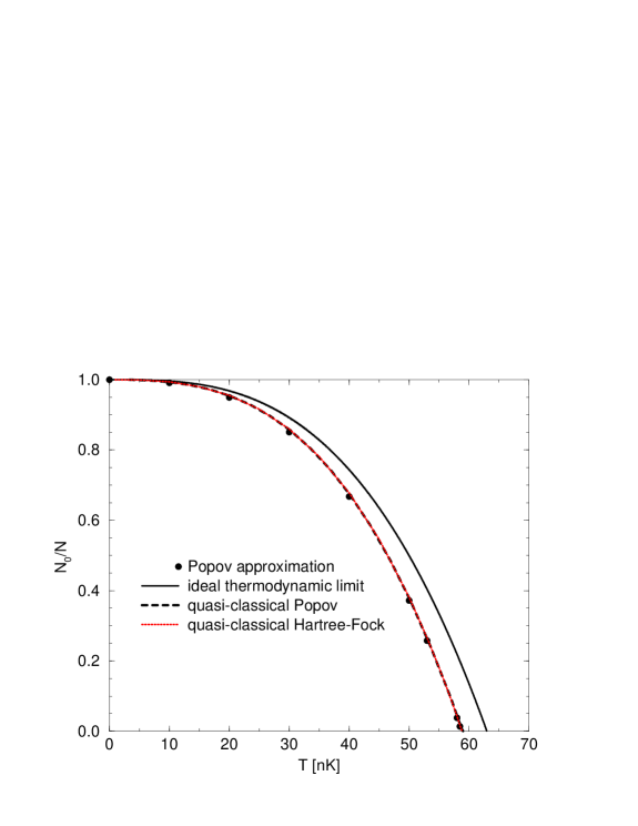
Figure 2: Condensate fraction vs temperature for $10^{3}$ ⁷Li atoms.

In Fig. 2 we plot the condensate fraction $N_{0}/N$ versus the temperature $T$. In this figure we include also the quasi-classical approximation of the Popov and Hartree method and the curve of the ideal gas in the thermodynamic limit. We observe that the quasi-classical Popov approximation, for which the classical energy reads $E({\bf p},{\bf r})=\sqrt{\big{[}{\bf p}^{2}/(2m)+U({\bf r})+2gn({\bf r})\big{]}^{2}+g^{2}n_{0}({\bf r})}$ (see also [20]), gives accurate results for the condensate fraction at all temperatures here considered.

Now we analyze a total number of atoms near the critical threshold $N_{c}\simeq 1260$, at which there is the collapse of the condensate. We use the quasi-classical Popov approximation to evaluate the critical threshold $N_{c}$ as a function of the temperature.

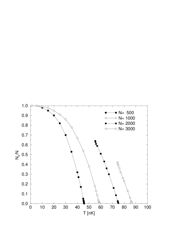
Figure 3: Condensate fraction vs temperature for different numbers of ⁷Li atoms. Results obtained with the quasi-classical Popov approximation.

In Fig. 3 we plot the condensate fraction as a function of the temperature $T$ for different numbers of ⁷Li atoms. By increasing the temperature it is possible to put a larger number of atoms in the trap but the metastable condensate has a decreasing number of atoms. Also the critical number $N_{0}^{c}$ of condensed atoms decreases by increasing the temperature. These results, obtained with the quasi-classical Popov approximation, show that, when $\omega=878$ Hz, for $N<N_{c}=1260$ the system is always metastable and it has a finite condensate fraction for $0\leq T<T_{{}_{BEC}}$, where $T_{BEC}$ is the BEC transition temperature. For $N>N_{c}$ the system is metastable only for temperatures that exceed a critical value $T_{c}$ and it has a finite condensate fraction for $T_{c}<T<T_{{}_{BEC}}$ [20].

We have seen that when the condensate fraction is only few percents then $\tilde{n}({\bf 0})/n_{0}({\bf 0})$ becomes sufficiently large and the BEC cannot take place anymore. Thus, our calculations suggest that there should be a critical temperature $T^{*}$ beyond which the BEC transition is inhibited, independently of the number of atoms in the trap. Obviously, $T_{c}$ and $T_{{}_{BEC}}$ are functions of $N$. Such temperatures, and also the critical parameter $N_{c}$, are functions of the trap geometry, namely the frequency $\omega$, and of the scattering length $a$ [20].

Finally, we observe that our calculations could be useful to select experimental conditions for which a fraction of condensed ⁷Li atoms is detectable at thermal equilibrium.

4 Bose gas of Hydrogen atoms

BEC has been also achieved with atomic Hydrogen confined in a Ioffe-Pritchard trap [10]. That is an important result because Hydrogen properties, like interatomic potentials and spin relaxation rates, are well understood theoretically. The s-wave scattering length of the Hydrogen is very low ($a=0.0648$ nm) and, compared with other atomic species, the condensate density is high, even for small condensate fractions. Moreover, due to hydrogen’s small mass, the BEC transition occurs at higher temperatures than previously observed.

We analyze the thermodynamical properties of the trapped Hydrogen gas by using the quasi-classical Hartree approximation. This approach is justified by the very large number of atoms (about $10^{10}$) in the trap and by the relatively high temperatures involved (order of $\mu$K). Our detailed theoretical study of the hydrogen thermodynamics can give useful informations for future experiments with a better optical resolution and a larger condensate fraction [22].

In the experiment reported in [10], the axially symmetric magnetic trap is modelled by the Ioffe-Pritchard potential

$$U(\rho,z)=\sqrt{(\alpha\rho)^{2}+(\beta z^{2}+\gamma)^{2}}-\gamma\;,$$ (34)

where $\rho$ and $z$ are cylindrical coordinates and the parameters $\alpha$, $\beta$ and $\gamma$ can be calculated from the magnetic coil geometry. In particular, for small displacements, the radial oscillation frequency is $\omega_{\rho}=\alpha/\sqrt{m\gamma}=2\pi\times 3.90$ kHz, the axial frequency is $\omega_{z}=\sqrt{2\beta/m}=2\pi\times 10.2$ Hz and $\gamma/k_{B}=35$ $\mu$K [10].

It is important to observe in the experiments with atomic Hydrogen, the gas is dilute ($na^{3}<<1$) but also strongly interacting because $Na/a_{h}>>1$, where $a_{h}=(\hbar/m\omega_{h})^{1/2}$ with $\omega_{h}=(\omega_{\rho}^{2}\omega_{z})^{1/3}$. It follows that the kinetic term of the finite-temperature Gross-Pitaevskii equation (18) can be safely neglected and one gets the Thomas-Fermi condensate density

$$n_{0}({\bf r})={1\over g}\left[\mu-U({\bf r})-2g\tilde{n}({\bf r})\right]\;,$$ (35)

in the region where $\mu>U({\bf r})+2gn_{T}({\bf r})$, and $n_{0}({\bf r})=0$ outside. In practice, we study the BEC thermodynamics by solving self-consistently the previous equation and Eq. (31).

Figure 4: BEC transition temperature $T_{c}$ versus number $N$ of hydrogen atoms. Comparison between harmonic and Ioffe-Pritchard trapping potential.

In Fig. 4 we compare the BEC transition temperature $T_{c}^{0}$ of the Ioffe-Pritchard potential with the analytic formula $T_{c}^{0,H}=0.94\hbar\omega_{h}N^{1/3}/k_{B}$, that is exact in the thermodynamic limit for the harmonic potential. Fig. 4 shows that, for a large number of atoms, $T_{c}^{0,H}$ exceeds $T_{c}^{0}$. In particular, for $N=2\cdot 10^{10}$ the relative difference is more than $41\%$. This strong effect is due to the larger density of states in the Ioffe-Pritchard trap.

The role of the interatomic interaction on the transition temperature $T_{c}$ is very small. In Fig. 4 one observes that the repulsive interaction reduces $T_{c}$ both in harmonic and Ioffe-Pritchard traps. This effect is of the order of $0.1$ $\mu$K.

Figure 5: Condensate fraction $N_{0}/N$ as a function of temperature $T$. $N$ interacting hydrogen atoms in the Ioffe-Pritchard trap.

In Fig. 5 we plot the condensate fraction $N_{0}/N$ as a function of temperature for $N=10^{8}$, $10^{9}$ and $10^{10}$ atoms. As previously stated, such curves could be a useful guide for future experiments with a better optical resolution and a larger condensate fraction (further details can be found in [22]).

5 Thermal Field Theory for Fermions

The Heisenberg equation of motion of the fermionic field operator ${\hat{\psi}}_{\sigma}({\bf r},t)$, which describes a non-relativistic system of confined and interacting identical atoms in the hyperfine state $\sigma$, is given by

$$i\hbar{\partial\over\partial t}{\hat{\psi}}_{\sigma}({\bf r},t)=\Big{[}-{\hbar^{2}\over 2m}\nabla^{2}+U({\bf r})\Big{]}{\hat{\psi}}_{\sigma}({\bf r},t)+$$

$$+\sum_{\sigma^{\prime}}\int d^{3}{\bf r}^{\prime}{\hat{\psi}}_{\sigma^{\prime}}^{+}({\bf r}^{\prime},t)V_{\sigma^{\prime}\sigma}({\bf r},{\bf r}^{\prime}){\hat{\psi}}_{\sigma^{\prime}}({\bf r}^{\prime},t){\hat{\psi}}_{\sigma}({\bf r},t)\;,$$ (36)

where $m$ is the mass of the atom, $U({\bf r})$ is the confining external potential and $V_{\sigma^{\prime}\sigma}({\bf r},{\bf r}^{\prime})$ is the interatomic potential [16].

The Bosonic field operator must satisfy the following equal-time anti-commutation rules

$$[{\hat{\psi}}_{\sigma^{\prime}}^{+}({\bf r}^{\prime},t),{\hat{\psi}}_{\sigma}({\bf r},t)]_{+}=\delta_{\sigma^{\prime}\sigma}\delta^{3}({\bf r}^{\prime}-{\bf r})\;,$$ (37)

$$[{\hat{\psi}}_{\sigma^{\prime}}({\bf r}^{\prime},t),{\hat{\psi}}_{\sigma^{\prime}}({\bf r},t)]_{+}=[{\hat{\psi}}_{\sigma^{\prime}}^{+}({\bf r}^{\prime},t),{\hat{\psi}}_{\sigma}^{+}({\bf r},t)]_{+}=0\;,$$ (38)

where $[{\hat{A}},{\hat{B}}]_{+}={\hat{A}}{\hat{B}}+{\hat{B}}{\hat{A}}$.

When the density of the atomic cloud is such that the scattering length and the range of the interatomic interaction are less than the average interatomic distance, the true interatomic potential can be approximated by a local pseudo-potential

$$V_{\sigma^{\prime}\sigma}({\bf r},{\bf r}^{\prime})=g_{\sigma^{\prime}\sigma}\delta^{3}({\bf r}-{\bf r}^{\prime})\;,$$ (39)

where $g_{\sigma^{\prime}\sigma}={4\pi\hbar^{2}a_{\sigma^{\prime}\sigma}/m}$ is the scattering amplitude and $a_{\sigma^{\prime}\sigma}$ is the s-wave scattering length. The s-wave scattering between Fermions in the same hyperfine state is inhibited ($a_{\sigma\sigma}=0$) due to the Pauli principle. Nevertheless, the effect of interaction could be very effective for a Fermi vapor with two or more hyperfine states. Thus, in the grand canonical ensemble, the equation of motion of the field operator, which describes a dilute fermi gas with atoms in different hyperfine states, can be written as

$$i\hbar{\partial\over\partial t}{\hat{\psi}}_{\sigma}({\bf r},t)=\Big{[}-{\hbar^{2}\over 2m}\nabla^{2}+U({\bf r})-\mu\Big{]}{\hat{\psi}}_{\sigma}({\bf r},t)+\sum_{\sigma^{\prime}}g_{\sigma^{\prime}\sigma}{\hat{\psi}}_{\sigma^{\prime}}^{+}({\bf r},t){\hat{\psi}}_{\sigma^{\prime}}({\bf r},t){\hat{\psi}}_{\sigma}({\bf r},t)\;,$$ (40)

while in the case of a dilute Fermi gas of atoms in a unique hyperfine state, the previous equation is simply

$$i\hbar{\partial\over\partial t}{\hat{\psi}}({\bf r},t)=\Big{[}-{\hbar^{2}\over 2m}\nabla^{2}+U({\bf r})-\mu\Big{]}{\hat{\psi}}({\bf r},t)\;.$$ (41)

This is the equation of motion of an ideal fermi gas in an external trapping potential.

For an ideal Fermi gas in external potential the Fermionic field can be expandend in the following way

$${\hat{\psi}}({\bf r},t)=\sum_{j}u_{j}({\bf r})e^{-iE_{j}t/\hbar}{\hat{a}}_{j}\;,$$ (42)

where $u_{j}({\bf r})$ is the single-particle eigenfunction with eigenvalue $\epsilon_{j}$ and ${\hat{a}}_{j}$ is the lowering Fermi operator of the single-particle eigenstate $|j\rangle$. The thermal spatial density is given by

$$n({\bf r})=\langle{\hat{\psi}}^{+}({\bf r},t){\hat{\psi}}({\bf r},t)\rangle=\sum_{j}|u_{j}({\bf r})|^{2}\langle{\hat{a}}^{+}_{j}{\hat{a}}_{j}\rangle\;,$$ (43)

with

$$\langle{\hat{a}}^{+}_{j}{\hat{a}}_{j}\rangle={1\over e^{E_{j}/kT}+1}$$ (44)

the Fermi factor at temperature $T$. In the quasi-classical approximation one uses the classical single-particle energy $E({\bf p},{\bf r})={\bf p}^{2}/(2m)+U({\bf r})$ instead of the quantum energy $E_{j}$. In this way the previous formula becomes

$$n({\bf r})=\int{d^{3}{\bf p}\over(2\pi\hbar)^{3}}{1\over e^{(E({\bf p},{\bf r})-\mu)/kT}+1}={1\over\lambda^{3}}\;f_{3/2}\left(e^{-(U({\bf r})-\mu)/kT}\right)\;,$$ (45)

where $\lambda=(2\pi\hbar^{2}/mk_{B}T)^{1/2}$ is the thermal length and

$$f_{n}(z)={1\over\Gamma(n)}\int_{0}^{\infty}dx{x^{n-1}\over z^{-1}e^{x}+1}\;,$$ (46)

with $\Gamma(x)$ the factorial function. Note that for $|z|<1$ one has $f_{n}(z)=\sum_{i=1}^{\infty}(-1)^{i+1}z^{i}/i^{n}$. Moreover, by using $g_{n}(z)=-f_{n}(-z)$ instead of $f_{n}(z)$, one finds the spatial distribution of the ideal Bose gas in external potential. In the limit of zero temperature, with $\mu=E_{F}$ the Fermi energy, the quasi-classical spatial distribution is given by the Thomas-Fermi approximation

$$n({\bf r})=(2m)^{3/2}/(6\pi^{2}\hbar^{3})\left(E_{F}-U({\bf r})\right)^{3/2}\Theta\left(E_{F}-U({\bf r})\right)\;,$$ (47)

where $\Theta$ is the Heaviside step function [17].

6 Fermi gas of Potassium atoms

In 1999 the Fermi quantum degeneracy has been obtained with dilute vapors of laser-cooled ⁴⁰K atoms confined in a magnetic trap [13]. In that experiment, to favor the evaporative cooling, a ⁴⁰K Fermi vapor in two hyperfine states is used. When the system is below the Fermi temperature, one hyperfine component is removed and it remains a trapped quasi-ideal degenerate Fermi gas. The s-wave scattering between fermions in the same hyperfine state is inhibited due the Pauli principle. It follows that at low temperature the dilute Fermi gas, in a fixed hyperfine state, is practically ideal. Nevertheless, the effect of interaction could be very effective for a Fermi vapor with two or more hyperfine states.

In the case of a harmonic external potential

$$U({\bf r})={1\over 2}m(\omega_{1}^{2}x^{2}+\omega_{2}^{2}y^{2}+\omega_{3}^{2}z^{2})\;,$$ (48)

one finds the Fermi density profile by using the Eq. (43) and the eigenfunctions $u_{n_{1}n_{2}n_{3}}({\bf r})$ of the harmonic oscillator

$$n({\bf r})=\sum_{n_{1}n_{2}n_{3}=0}^{\infty}{|u_{n_{1}n_{2}n_{3}}({\bf r})|^{2}\over e^{\beta\hbar(\omega_{1}(n_{1}+1/2)+\omega_{2}(n_{2}+1/2)+\omega_{3}(n_{3}+1/2)-\mu)}+1}\;.$$ (49)

Because the Fermi gas is ideal, one has $u_{n_{1}n_{2}n_{3}}({\bf r})=u_{n_{1}}(x)u_{n_{2}}(y)u_{n_{3}}(z)$, where $\phi_{n}(x)$ is the eigenfuction of a 1D harmonic oscillator with frequency $\omega$ and quantum number $n$. This eigenfunction can be found by means of the recursion relation

$$u_{n}(x)={1\over\sqrt{n}}\Big{[}\sqrt{2}a_{h}xu_{n-1}(x)-\sqrt{n-1}u_{n-2}(x)\Big{]}\;,$$ (50)

where $u_{0}(x)=a_{h}^{1/2}\pi^{1/4}e^{-a_{h}^{2}x^{2}/2}$ and $u_{1}(x)=\sqrt{2}a_{h}xu_{0}(x)$, with $a_{h}=\sqrt{\hbar/(m\omega)}$.

Figure 6: Density profiles for an ideal Fermi gas in a 1D harmonic trap. Temperature: $kT/\hbar\omega=10^{-3}$; at this temperature the results coincide with zero-temperature ones. $N$ is the number of Fermions. Lengths in units $a_{h}=(\hbar/m\omega)^{1/2}$ and densities in units $a_{h}^{-3}$.

In the quasi-1D case, namely a cigar-shaped gas where $\omega_{1}=\omega_{2}>>\omega_{3}$, the shell effects are strongly enhanced. In Fig. 6 we plot the density profile of a 1D ideal Fermi gas in harmonic potential as a function of the number $N$ of particles at $kT/\hbar\omega=10^{-3}$. We have verified that at this temperature the density profiles coincide with the zero-temperature ones. The results are obtained by numerically evaluating expressions (49) and (50) in the 1D case. The local maxima, whose number grows with $N$, are clearly visible for a small number of particles.

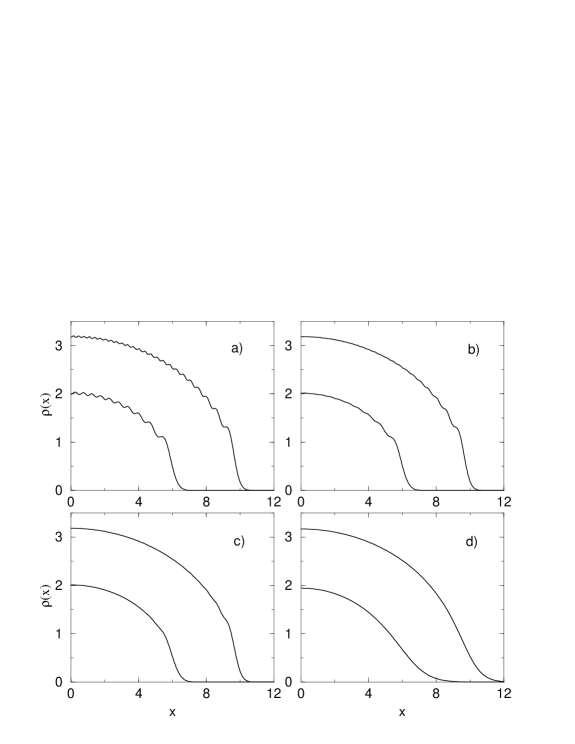
Figure 7: Density profiles for an ideal Fermi gas in a 1D harmonic trap at finite temperature, with $N=20$ and $50$. $N$ is the number of Fermions. a) $kT/\hbar\omega=1/10$; b) $kT/\hbar\omega=1/2$; c) $kT/\hbar\omega=1$; d) $kT/\hbar\omega=5$. Units as in Figure 6.

In Fig. 7 we show the density profiles with $20$ and $50$ particles as a function of temperature. Remarkably, the local peaks are no more distinguishable for temperatures well below the Fermi temperature $T_{F}=N\hbar\omega/k$. Thus, to see spatial shell effect on the 1D density profile, the system should be at temperatures lower than $T_{F}$ by one or two orders of magnitude.

The problem of a dilute Fermi vapor with $M$ hyperfine states (components), can be studied by using the mean-field approximation and the quasi-classical formula. The spatial density profile $n_{\sigma}({\bf r})$ of the $\sigma$-th component in a $M$-component Fermi vapor can be written as

$$n_{\sigma}({\bf r})={1\over\lambda^{3}}f_{3/2}\left(e^{\left(\mu_{\sigma}-U({\bf r})-\sum_{\sigma^{\prime}=1}^{M-1}g_{\sigma^{\prime}\sigma}n_{\sigma^{\prime}}({\bf r})\right)/kT}\right)\;,$$ (51)

where $\sigma=1,...,M$, $\mu_{\sigma}$ is the chemical potential of the $\sigma$-th component, and $g_{\sigma^{\prime}\sigma}=4\pi\hbar^{2}a_{\sigma^{\prime}\sigma}/m$, with $a_{\sigma^{\prime}\sigma}$ the s-wave scattering length between $\sigma^{\prime}$-th and $\sigma$-th component ($a_{\sigma\sigma}=0$). Thus, the effect of the other $M-1$ Fermi components on the $\sigma$-th component is the appearance of a mean-field effective potential.

We numerically solve the set of equations (51) with a self-consistent iterative procedure. If the components of the Fermi vapor are non-interacting then they can occupy the same spatial region. Instead, if they are strongly interacting (repulsive interaction) there will be a phase-separation, i.e., the Fermi components will stay in different spatial regions.

When two components have the same number of particles, the onset of phase-separation is also an example of spontaneous symmetry breaking. In fact, if the chemical potentials $\mu_{i}$ of the two components are equal, Eq. (51) always admits a symmetric solution $n_{1}({\bf r})=n_{2}({\bf r})$. However, for particle number $N$ larger than a threshold $N_{c}$ the solution bifurcates and a pair of symmetry breaking solutions appears (see [23]).

Figure 8: Density profiles of the ⁴⁰K vapor with three components (solid, dotted and dashed lines) in a 3D isotropic harmonic trap ($\omega=450$ Hz). $N=0.5\cdot 10^{7}$ atoms for each component. Different values of the scattering length $a$ ($a_{0}$ is the Bohr radius). Temperature $T=0.5T_{F}$ ($T_{F}=1.07$ $\mu$K). Lengths in units $a_{h}=(\hbar/m\omega)^{1/2}$ and densities in units $a_{h}^{-3}$.

Phase-separation also appears in a Fermi vapor with three or more components. In Figure 8 we plot the density profiles of the ⁴⁰K Fermi vapor with three components in a 3D isotropic harmonic potential. In this case we numerically solve Eq. (51) with $a_{12}=a_{13}=a_{23}=a$. The Figure shows that also for three components the phase-separation and the apparence of spatial shells are regulated by the scattering length.

A Fermi vapor with more components has the same behavior. In particular, we have recently shown [23] that the critical density of fermions at the origin, which gives rise to the phase-separation, does not depend on the number of Fermi component and on the properties of the trap; moreover we have found, by using standard bifurcation theory, that such a density is given by $n_{c}({\bf 0})=\pi/(48a^{3})$, where $a$ is the s-wave scattering length.

7 Conclusions

We have shown that non-relativistic quantum field theory is extremely useful to explain results of recent experiments with dilute alkali-metal atoms at ultra-low temperatures and to predict new quantum phenomena not yet experimentally observed. By studying these systems, sophisticated theoretical concepts, like order parameter, spontaneous symmetry breaking and off-diagonal long-range order, find a clear correspondence in measurable physical quantities. Finally, it is important to stress the role of the quasi-classical approximation, which is not only useful in computations but is also a giude for a deeper understanding of physical problems.

References

[1] Bose S N, 1924 Z. Phys. 26 178

[2] Einstein A, 1924 Preussische Akademie der Wissenshaften 22 261; 1925 1 3; 1925 3 18

[3] London F, 1938 Nature 141 643; 1938 Phys. Rev. 54 947; 1938 J. Phys. Chem. 43 49

[4] Tisza L, 1938 Nature 141 913; 1940 Journal de Physique et Radium 1 164 350

[5] Landau L D, 1941 J. Phys. U.S.S.R. 5 71; 1947 11 91

[6] Bogoliubov N N, 1947 J. Phys. U.S.S.R. 11 23; Beliaev S T, 1958 Sov. Phys. JETP 7 299; Popov V N, 1987 Functional Integrals and Collective Modes, Cambridge University Press: Cambridge

[7] Anderson M H, Ensher J R, Matthews M R, Wieman C E, and Cornell E A, 1995 Science 269 189

[8] Davis K B, Mewes M O, Andrews M R, van Druten N J, Drufee D S, Kurn D M, and Ketterle W, 1995 Phys. Rev. Lett. 75 3969

[9] Bradley C C, Sackett C A, Tollett J J, and Hulet R G, 1995 Phys. Rev. Lett. 75 1687

[10] D.G. Fried D G, Killian T C, and Kleppner D, 1998 Phys. Rev. Lett. 81 3811

[11] Gross E P, 1961 Nuovo Cimento 20 454; 1963 J. of Math. Phys. 2 195; L.P. Pitaevskii, 1961 Sov. Phys. JETP 13 451

[12] Chu S, Cohen-Tannouji C, and Phillips W D, 1997 Nobel Prize in Physics

[13] Fermi E, 1926 Z. Physik 36 902; Dirac P A M, 1926 Proc. Roy. Soc. A 112 661 (1926)

[14] Fierz M, 1939 Helv. Phys. Acta 12 3; Pauli W, 1940 Phys. Rev. 58 716

[15] DeMarco B and Jin D S, 1999 Science 285 1703

[16] Huang K, 1987 Statistical Mechanics, John Wiley: New York; Fetter A L and Walecka J D, 1971 Quantum Theory of Many-Particle Systems, Mc Graw-Hill: Boston

[17] Salasnich L, 2000 J. Math. Phys. 41 8016

[18] Goldstone J, 1961 Nuovo Cimento 19 154; Anderson P W, 1966 Rev. Mod. Phys. 38 298

[19] Penrose O, 1951 Phil. Mag. 42 1373; Penrose O and Onsager L, 1956 Phys. Rev. 104 576

[20] Pozzi B, Salasnich L, Parola A, and Reatto L, 2000 J. Low Temp. Phys. 119 57

[21] Salasnich L, 1997 Mod. Phys. Lett. B 11 1249; 1998 12 649

[22] Pozzi B, Salasnich L, Parola A, and Reatto L, 2000 Eur. Phys. J. D 11 367

[23] Salasnich L, Pozzi B, Parola A, and Reatto L, 2000 J. Phys. B 33 3943