Dynamic critical properties of the vortex–glass transition derived from angular-dependent properties of La_2-xSr_xCuO₄ films

Abstract

We present resistivity data on a high-quality La_2-xSr_xCuO_4-δ film measured in a magnetic field of 1 T applied at an angle $\delta$ to the $c$ axis. Using these data, the influence of the orientation of the magnetic field and the effective mass anisotropy on the vortex–glass transition can be studied. The variation of $\delta$ for a fixed magnitude of the magnetic field allows us to investigate the critical properties of interest, including the 2D-to-3D crossover and the 3D vortex glass-to-fluid transition, as the temperature is decreased. The data are well described by the scaling theory for the d.c. resistivity of an anisotropic superconductor in a magnetic field applied at an angle $\delta$ to the $c$ axis. This scaling includes the critical properties close to and at the vortex–glass transition. The main results include (i) evidence of a Kosterlitz–Thouless transition in zero field, and (ii) a 2D-to-3D crossover at $H=1$ T as the temperature is decreased below the zero-field transition temperature, leading to the vortex fluid-to-vortex glass transition in D = 3 characterized by the dynamic critical exponent $z\approx 5.7$.

I Introduction

The critical dynamics of the vortex system in cuprate superconductors is strongly affected by the combined effect of pinning, thermal fluctuations, anisotropy, and dimensionality.[1] Thermal fluctuations are responsible for the existence of a first-order vortex lattice melting transition in clean systems. In the presence of disorder, however, the long-range order of the vortex lattice is destroyed and the vortex solid becomes a glass. The vortex fluid-to-glass transition appears to be a second-order transition, signaled by the vanishing of the zero-frequency resistance in the vortex-glass phase. A schematic sketch of the phase diagram is shown in Fig. 1. By lowering the magnetic field at temperatures below $T_{c}$ ($H=0$) the material undergoes the vortex liquid-to-vortex glass or Bose glass transition at $H=H_{g}$ (path 3). Similarly, at constant field, the transition occurs at $T_{g}<T_{c}$ (path 2) for lower temperatures.

In the Anderson–Kim flux-creep model,[2] and extensions thereof[3] that include pinning effects, the collective effects of vortices are neglected. In these models, the linear resistance is predicted to drop rapidly upon cooling (path 2) but always remains nonzero. On the other hand, there is considerable evidence of a nearly continuous vortex melting transition. In the presence of pinning, however, Larkin and Ovchinnikov [4] have shown that the long-range order of the vortex lattice is destroyed in all spatial dimensions smaller than four. Hence in two and three dimensions pinning should dominate. Following the work of Ebner and Stroud,[5] Fisher[6] and Fisher, Fisher and Huse[7] have postulated a continuous vortex–glass transition with infinite conductivity in the glass phase. Experimental evidence of this transition has been obtained from the critical behavior of transport properties for magnetic fields applied parallel to the $c$ axis.[8, 9, 10, 11, 12, 13, 14]

In this study, we consider the full range of the angle $\delta$ between the applied magnetic field and the $c$ axis. We present resistivity data on a high-quality La_2-xSr_xCuO₄ film with $x\approx 0.1$ in a magnetic field of 1 T applied at an angle $\delta$ to the $c$ axis. This allows us to study the influence of the orientation of the magnetic field and the effective mass anisotropy on the glass transition. By varying $\delta$ for a fixed magnitude of the magnetic field, we have been able to investigate the critical properties of interest, including the 2D-to-3D crossover and the 3D vortex glass-to-fluid transition. Noting that in this film disorder is much stronger than in high-quality single crystals, we do not consider the Bragg–glass transition.[16]

The paper is organized as follows. In Sec. II we first summarize the scaling theory for the d.c. resistivity of an isotropic superconductor. This formalism is then extended to account for anisotropy and an angle $\delta$ between magnetic field and the $c$ axis. The scaling includes the critical properties close to and at the vortex–glass transition. Section III contains the experimental details, results and their analysis. The main results include (i) evidence of a Kosterlitz–Thouless transition in zero field; (ii) a 2D-to-3D crossover at $H=1$ T as the temperature is lowered below the zero-field transition temperature, leading to the vortex fluid-to-vortex glass transition in D = 3 characterized by the dynamic critical exponent $z_{g}\approx 5.7$.

II Scaling Theory

A continuous phase transition from the superconducting to the normal phase allows a general formulation of the scaling at and near such a transition.[15] In an isotropic system the fluctuation contribution to the conductivity adopts the scaling form

$$\sigma^{F}\propto\xi^{2+z_{g}-{\rm D}}{\cal F}({\cal Z}),\ \ {\cal Z}=\frac{H\xi^{2}}{\Phi_{0}},$$ (1)

where $\xi$ is the correlation length, $H$ the magnetic field, $z$ the dynamic critical exponent, and ${\cal F}({\cal Z})$ a universal scaling function. Its form will be discussed later. Close to the vortex–glass transition the correlation length diverges with an exponent $\nu_{g}$ as[6]

$$\xi=\xi_{T,0}\left(\frac{T-T_{g}}{T_{g}}\right)^{-\nu_{g}}\text{ and }\ \xi=\xi_{H,0}\left(\frac{H-H_{g}}{H_{g}}\right)^{-\nu_{g}}$$ (2)

along paths 2 and 3 (see Fig. 1), respectively. Hence it follows that the conductivity will diverge along the phase-transition line

$${\cal Z}={\cal Z}_{g}.$$ (3)

In this context it is important to recognize that ${\cal Z}_{g}$ is a number that locates the transition. Close to the zero-field transition of a bulk sample at $T_{c}$ ($H=0$), the isotropic 3D-$XY$ fluctuations are expected to dominate. In this case the phase-transition line in Fig. 1 follows from

$${\cal Z}_{g}=\frac{H_{g}\xi^{2}(T)}{\Phi_{0}},\ \ \xi(T)=\xi_{0}\left(\frac{T_{c}(H=0)-T}{T_{c}(H=0)}\right)^{-\nu},\;\nu\approx 2/3\,,$$ (4)

so that

$$H_{g}=\frac{{\cal Z}_{g}\Phi_{0}}{\xi_{0}^{2}}\left(\frac{T_{c}(H=0)-T}{T_{c}(H=0)}\right)^{2\nu}.$$ (5)

At ${\cal Z}_{g}$ the scaling function exhibits singular behavior, signaling the occurrence of the transition. Its critical behavior is governed by the glass correlation length [Eq. (2)] rewritten as

$$\xi\propto\left(\frac{T-T_{g}}{T_{g}}\right)^{-\nu_{g}}\propto\left(\frac{H-H_{g}}{H_{g}}\right)^{-\nu_{g}}\propto\left({\cal Z}-{\cal Z}_{g}\right)^{-1/2}.$$ (6)

Combining Eqs. (1), (3) and (6), we find that the conductivity will diverge along path 2 (see Fig. 1) as

$$\sigma^{F}\propto t^{-\nu_{g}(2+z-D)}{\cal F}({\cal Z}_{g}),\ \ t=\frac{T-T_{g}}{T_{g}}$$ (7)

and along path 3 (Fig. 1) as

$$\sigma^{F}\propto\left(\frac{H-H_{g}}{H_{g}}\right)^{-\nu_{g}(2+z_{g}-D)}{\cal F}({\cal Z}_{g}).$$ (8)

However, along path 1, where $T=T_{c}(H=0)$, the conductivity is finite for any $H\neq 0$. Rewriting the conductivity [Eq. (1)] in the form

$$\sigma^{F}\propto\xi^{2+z-D}{\cal F}({\cal Z})=\left(\frac{{\cal Z}\Phi_{0}}{H}\right)^{(2+z-D)/2}{\cal F}({\cal Z}),$$ (9)

we see that it scales as

$$\sigma^{F}\propto\left(\frac{\Phi_{0}}{H}\right)^{(2-D+z)/2},\ \ {\cal F}({\cal Z})\propto{\cal Z}^{-(2+z-D)/2}.$$ (10)

The dynamic critical exponent $z$ is expected to differ from that entering the normal-to-vortex glass transition ($z_{g}$). Indeed, as $H$ is lowered one approaches in this case the zero-field transition point.

At the normal-to-vortex glass transition, the conductivity is supposed to be infinite. This requires the scaling form

$$\sigma^{F}\propto({\cal Z}-{\cal Z}_{g})^{-(2+z_{g}-D)/2}\ .$$ (11)

Indeed, according to Eqs. (1) and (6) we have

$$\sigma^{F}\propto\xi^{2+zg-D}{\cal F}({\cal Z}),\ \ \ \ \xi\propto({\cal Z}-{\cal Z}_{g})^{-1/2},$$ (12)

so that close to criticality (${\cal Z}={\cal Z}_{g})$,

$$\sigma^{F}\propto({\cal Z}-{\cal Z}_{g})^{-(2+z_{g}-D)/2}{\cal F}({\cal Z}_{g}).$$ (13)

For anisotropic superconductors and in particular for arbitrary orientation of the applied field with respect to the $c$ axis, various expressions have to be modified.

III Bulk superconductor (D = 3) with uniaxial anisotropy

For a bulk superconductor with uniaxial anisotropy the scaling variable adopts the form[14]

$${\cal Z} = {\cal Z}(H,T)\ {\cal Z}(\gamma,\delta),\ \ \ \ \ \ \gamma=\sqrt{\frac{M_{\bot}}{M_{\|}}}$$ (14)

$${\cal Z}(H,T) = \frac{\xi_{\|}^{2}H}{\Phi_{0}},\$$ (15)

$${\cal Z}(\gamma,\delta) = \left(\cos^{2}(\delta)+\frac{1}{\gamma^{2}}\sin^{2}(\delta)\right)^{1/2}\,,$$ (16)

where $\delta$ is the angle between the $c$ axis and the magnetic field, and $\xi_{\|}$ is the correlation length in the $ab$ plane (perpendicular to the $c$ axis). Here $\gamma$ measures the anisotropy of the effective mass parallel ($ab$) and perpendicular ($a$) to the layers. Thus the in-plane conductivity [Eq. (1)] adopts in the bulk the scaling form

$$\sigma^{F}\propto\xi_{\|}^{z_{g}-1}{\cal F}({\cal Z})=\xi_{\|}^{z_{g}-1}{\cal F}\left({\cal Z}(H,T)\ {\cal Z}(\gamma,\delta)\right).$$ (17)

Hence, close to criticality, the $\delta$-dependent conductivity, $\sigma^{F}(\delta)$, measured at constant field $H$ and temperature $T$ plotted versus ${\cal Z}(\gamma,\delta)$ should fall on a single curve. In anisotropic bulk systems this offers the opportunity to probe the scaling function for fixed temperature and magnetic field in the domain

$$\frac{{\cal Z}(H,T)}{\gamma}\leq{\cal Z}\leq{\cal Z}(H,T).$$ (18)

Supposing that 3D-$XY$ fluctuations dominate close to $T=T_{c}(H=0)$, the vortex–glass transition line defined by ${\cal Z=Z}_{g}$ [Eq. (3)] is then given by the angular-dependent expression

$$H_{g}(\delta)=\frac{{\cal Z}_{g}\Phi_{0}}{\xi_{\|,0}^{2}}\left(\frac{T_{c}(H=0)-T}{T_{c}(H=0)}\right)^{2\nu}\left(\cos^{2}(\delta)+\frac{1}{\gamma^{2}}\sin^{2}(\delta)\right)^{-1/2},\ \nu\approx 2/3.$$ (19)

We note that for $\delta=0$, $2\nu\approx 4/3$ turned out to be consistent with the data of Gammel et al. for YBa₂Cu₃O_7-δ single crystals.[9] At the normal-to-vortex glass transition, the conductivity is infinite.[7] According to Eq. (10) this implies

$$\sigma^{F}\propto({\cal Z}-{\cal Z}_{g})^{-(z_{g}-1)/2},$$ (20)

where

$${\cal Z}-{\cal Z}_{g} = \left({\cal Z}(H,T){\cal Z}(\gamma,\delta)-{\cal Z}_{g}\right)$$ (21)

$$= {\cal Z}(H,T)\left({\cal Z}(\gamma,\delta)-\frac{{\cal Z}_{g}}{{\cal Z}(H,T)}\right)$$ (22)

and hence

$$\sigma^{F}\propto{\cal Z}(H,T)^{-(z_{g}-1)/2}({\cal Z}(\gamma,\delta)-\widetilde{{\cal Z}}_{g})^{-(z_{g}-1)/2},\ \widetilde{{\cal Z}}_{g}=\frac{{\cal Z}_{g}}{{\cal Z}(H,T)}.$$ (23)

Thus the plot $\sigma^{F}(\delta)$ versus ${\cal Z}(\gamma,\delta)$ allows us to estimate the dynamic critical exponent $z_{g}$ directly. The prefactor depends on the magnetic field and temperature.

Along path 1 (see Fig. 1) the conductivity adopts a rather different scaling form. In analogy to Eq. (10),

$$\sigma^{F}\propto\left(\frac{\Phi_{0}}{H{\cal Z}(\gamma,\delta)}\right)^{(z-1)/2},\ {\cal F}({\cal Z})\propto{\cal Z}^{-(z-1)/2}.$$ (24)

It is important to recall that this dynamic critical exponent $z$ is expected to differ from that entering the normal-to-vortex glass transition $(z_{g})$. Indeed, as $H$ is lowered one approaches the zero-field transition point.

IV Thin films

In thin films of thickness $d$, 2D fluctuations dominate as long as

$$\xi_{c}\equiv\xi_{\bot}\geq d.$$ (25)

Here $\xi_{c}$ denotes the correlation length along the $c$ axis, which is perpendicular to the film. Approaching the Kosterlitz–Thouless transition [17] from above, the zero-field conductivity scales according to Eq. (1) as

$$\sigma^{F}\propto\xi^{z},$$ (26)

where $\xi$ is given by

$$\xi\propto\exp(b(T/T_{c}-1)^{-1/2}),\ \ T>T_{c}.$$ (27)

Accordingly, the resistivity scales as

$$\rho\propto\xi^{-z}\propto\exp(-zb(T/T_{c}-1)^{-1/2}),$$ (28)

and hence

$$(\ln\rho)^{-2}\propto T/T_{c}-1.$$ (29)

In D = 2 and a finite applied magnetic field, the scaling variable ${\cal Z}$ entering the expression for the conductivity [Eq. (1)] adopts the form[18]

$${\cal Z} = {\cal Z}(H,T)\ {\cal Z}(H,\delta)$$ (30)

$${\cal Z}(H,T) = \frac{H^{1/2}\xi_{\|}}{\Phi_{0}^{1/2}},\$$ (31)

$${\cal Z(}H,\delta) = \left((|\cos(\delta)|+\frac{Hd^{2}}{12\Phi_{0}}\sin^{2}(\delta)\right)^{1/2}.$$ (32)

Accordingly, in a film of thickness $d$, angular-dependent conductivity measurements allow us to probe the scaling function for fixed temperature and magnetic field in the domain

$${\cal Z}(H,T)\left(\frac{Hd^{2}}{12\Phi_{0}}\right)^{1/2}\leq{\cal Z\leq Z}(H,T).$$ (33)

Comparing the angular dependence of the scaling variable for anisotropic bulk systems [Eq. (16)] with that of a sufficiently thin film [Eq. (32)], it is seen that they differ markedly around $\delta=\pi/2$. Indeed, ${\cal Z}(H,\delta)$ has a cusp at $\delta=\pi/2$, whereas ${\cal Z}(\gamma,\delta)$ is smooth. Moreover, ${\cal Z}(H,\delta)$ depends on the magnetic field. The cusp of ${\cal Z}(H,\delta)$ at $\delta=\pi/2$, modulo $\pi$ leads to a V-shaped structure around these angles in the resistivity and, together with the magnetic field dependence, allows an unambiguous determination of the effective dimensionality.

According to Eq. (1) the conductivity in the regime where 2D fluctuations dominate [Eq. (25)] then adopts the scaling form

$$\sigma^{F}\propto\xi^{z_{g}}{\cal F}({\cal Z})=\xi^{z_{g}}\ {\cal F}\left({\cal Z}(H,T)\ {\cal Z}(H,\delta)\right).$$ (34)

Hence close to criticality and for fixed $H$ and $T$, angular-dependent conductivity data $\sigma^{F}(\delta)$ plotted versus ${\cal Z}(H,\delta)$ should fall on a single curve. Experiments,[19] simulations,[20] and rigorous analytic arguments[21] revealed, however, that there is no vortex glass at finite $T$ in D = 2. Even though $T_{g}=0$, the correlation length diverges as $T\rightarrow 0$,

$$\xi\propto T^{-\nu_{g}},$$ (35)

which leads to observable consequences at finite temperatures. Moreover, as the transition is at $T=0$, the relaxation has an activated form and diverges as $T\rightarrow 0$. Formally this corresponds to $z_{g}=\infty$. To eliminate $z_{g}$ in Eq. (34) one can introduce the barrier $\Delta E(T)$ that a vortex has to cross in order to move a distance $\xi$. In this context one conventionally defines the barrier exponent $\psi$ by[22]

$$\Delta E(T)\propto\xi^{\psi}\propto T^{-\nu_{g}\psi},$$ (36)

in terms of which

$$\frac{1}{\tau}\propto\exp(-\Delta E/T)\propto\exp(-C/T^{1+\nu_{g}\psi}).$$ (37)

With the definition $\tau\propto\xi^{z}$ the afore-mentioned problem $(z_{g}=\infty)$ is resolved and the scaling form of the conductivity [Eq. (34)] reduces to

$$\sigma^{F}\propto\exp(C\xi^{\psi+1/\nu_{g}}){\cal F}({\cal Z})=\exp(C\xi^{\psi+1/\nu_{g}})\ {\cal F}\left({\cal Z}(H,T)\ {\cal Z}(H,\delta)\right).$$ (38)

Along path 1 (see Fig. 1), however, 2D-$XY$ fluctuations are expected to dominate. Here the conductivity exhibits, analogous to Eqs. (10) and (24), the power-law behavior

$$\sigma^{F}\propto\left(\frac{\Phi_{0}}{H}\right)^{z/2}{\cal Z}(\gamma,\delta)^{-z},\ \ {\cal F}({\cal Z})\propto{\cal Z}^{-z}.$$ (39)

V Results and Discussion

We have measured the angular dependence of the in-plane resistivity on a 120-Å-thick La_2-xSr_xCuO₄ film. The film was grown by molecular-beam epitaxy on a (001)-oriented LaSrAlO₄ substrate. Details of the sample preparation have been described elsewhere.[23] The angle-dependent resistivity measurements were performed with a commercial a.c. transport setup (quantum design measurement system) using the conventional four-point method.

In Fig. 2 we depict the zero-field temperature dependence of the La_2-xSr_xCuO₄ film. Included is the plot $(\ln\rho)^{{-2}}$ versus $T$. According to Eq. (29) it provides the estimate $T_{c}(H=0)\approx 36.74$ K for the Kosterlitz–Thouless transition temperature.

The angular dependence of the resistivity in a magnetic field of $H=1$ T is shown in Fig. 3 for different temperatures. The parameter $\delta$ is the angle between the magnetic field and the $c$ axis of the film.

For fixed $\delta$, the resistivity decreases with decreasing temperature. To provide some preliminary evidence of the vortex–glass transition in D = 3, we show in Fig. 4 $\rho(\delta=0)$ versus $T$ and $\rho^{1/4}$ versus $T$ [see Eq. (7)], assuming that[12]

$$\nu_{g}(2+z_{g}-D)=\nu_{g}(z_{g}-1)\approx 4.$$ (40)

One can see that $\rho^{1/4}$ is linearly dependent on $T$, which yields the estimate

$$T_{g}(\delta=0,H=1\;{\rm T})\approx 29.7\;{\rm K}.$$ (41)

Below $T_{c}(H=0)=36.74$ K, where at constant field and in D = 3 the vortex–glass transition is expected to occur, the angular dependence shown in Fig. 3 appears to be consistent with anisotropic 3D bulk behavior, whereas at higher temperatures a crossover to 2D behavior sets in, characterized by a sharp drop of the resistivity around 90^∘ and 270^∘.

To explore the 2D-$XY$ regime more quantitatively we consider $T=36.58$ K, which is close to $T_{c}(H=0)\approx$ 36.74 K, where the Kosterlitz–Thouless transition occurs (see Fig. 2). In this temperature regime and for sufficiently small magnetic fields, 2D fluctuations are expected to dominate and, according to Eq. (39), a simple power-law behavior is expected. Accordingly, a plot $\log_{10}\left(\rho\right)$ versus $\log({\cal Z}(H,\delta))$ providing an estimate for $z$ appears to be appropriate with

$$(Hd^{2})/(12\Phi_{0})=0.0058$$ (42)

for $d=120$ Å and $H=1$ T.  The plot shown in Fig. 5 points to the characteristic power law behavior valid in D = 2 and yields the estimate

$$z=3.96\pm 0.02,$$ (43)

This estimate differs from the value of $z=2$ expected from simple diffusion, and is closer to $z=5.6$, the value that emerges from a recent re-analysis of the experimental data for 2D superconductors, Josephson-junction arrays, and superfluids.[24]

Another manifestation of dominant 2D fluctuations, requiring $\xi_{c}\equiv\xi_{\bot}\geq d$, is shown in Fig. 6 in terms of $\rho$ versus $\delta$ around $\delta=90^{\circ}$ for $T=38.16$ K and $H=1$ T. Indeed, the characteristic V-shape clearly indicates the 2D scaling behavior in this temperature regime. From Fig. 3 it is seen, however, that the 2D behavior disappears as the temperature is lowered. In this context it should be noted that there are three important length scales in the problem: (i) the average distance between the vortices

$$l=\left(\frac{\Phi_{0}}{\pi H}\right)^{1/2}\approx 256\,{\rm\AA\/\;at\;1\;T};$$ (44)

(ii) the correlation length parallel to the layers, $\xi_{\|}$. The critical regime for the 3D vortex glass-to-normal transition requires, at the very least, that

$$\xi_{\|}\geq l,$$ (45)

which is thus more accessible in large fields; and (iii) the correlation length perpendicular to the layers, $\xi_{\bot}$. In experiments on films of thickness $d$, 3D critical behavior requires [Eq. (25)] that

$$\xi_{\bot}=\frac{\xi_{\|}}{\gamma}<d.$$ (46)

The absence of the characteristic 2D V-shape in the angular dependence of the resistivity around $\delta=90^{\circ}$ and 270^∘ and below $T=36$ K (see Fig. 3) suggests that in the regime considered here, condition (45) is satisfied. Indeed, from Fig. 7 it is seen that the resistivity appears to vanish below a certain value of the scaling variable. This suggests that in this temperature regime the 3D scaling form (23) for the normal-to-vortex glass transition applies, so that

$$\rho=a+b({\cal Z}(\gamma,\delta)-\widetilde{{\cal Z}}_{g})^{(z_{g}-1)/2},\ \widetilde{{\cal Z}}_{g}=\frac{{\cal Z}_{g}}{{\cal Z}(H,T)}$$ (47)

where ${\cal Z}(\gamma,\delta)$ is given by Eq. (16) and $a$ accounts for the residual resistivity. Here we used $\gamma\approx 20$, the value derived from magnetic torque measurements on bulk samples close to optimum doping.[25] The fit parameters are listed in Table I. At $\widetilde{{\cal Z}}_{g}\approx 0.45$ the resistivity approaches zero and vanishes below this threshold, signaling the vortex-glass phase. The resulting behavior of the angular-dependent resistivity is depicted in Fig. 8. Here the vortex-glass phase appears in the interval $65.95\leq\delta\leq 114.05^{\circ}$ (modulo $\pi$). In Table I we also included the estimates derived from the data taken at $T=33.1$, 33.6 and 34.1 K. The consistency of the estimates for $(z_{g}-1)/2$ and ${\cal Z}_{g}$ suggests that in the temperature regime considered here the 3D normal phase-to-vortex glass transition was attained at constant temperature and magnetic field by varying the orientation of the magnetic field.

Substantiation of this conclusion amounts to show that ${\cal Z}_{g}$ can be approached without violating the condition given by Eqs. (45) and (46). A rough estimate for ${\cal Z}_{g}$ is obtained using Eq. (19) with $\xi_{\|,0}\approx 30$ Å, $T_{c}(H=0)\approx 36.74$ K and $T_{g}(H=1\,{\rm T})\approx 29.7$ K [Eq. (41)], yielding ${\cal Z}_{g}\approx 0.039$. On the other hand, from ${\cal Z}(H,T)=(\xi_{\|}^{2}H)/\Phi_{0}$ we find ${\cal Z}(H=1\,{\rm T},\,T=33.1\,{\rm K})\approx 0.094$, using $\xi_{\|}=\xi_{\|,0}(1-33.1/36.74)^{-2/3}\approx 140$ Å for $\xi_{\|,0}\approx 30$ Å. Hence $\ \widetilde{{\cal Z}}_{g}(T=33.1\,{\rm K})={\cal Z}_{g}/{\cal Z}(H,T)\approx 0.41$, in remarkable agreement with the value listed in Table I. Moreover, considering

$${\cal Z}(\xi_{\|},\delta)={\cal Z}(H=1T,T){\cal Z}(\gamma,\delta)={\cal Z}_{g}=0.039$$ (48)

with ${\cal Z}(H,T)$ and ${\cal Z}(\gamma,\delta)$ given by Eq. (16), it is readily seen from Fig. 9 that in the interval $80^{\circ}\leq\delta\leq 110^{\circ}$, ${\cal Z}_{g}$ can be approached without violating condition (45). Moreover, noting that $\xi_{\bot}=\xi_{\|}/\gamma\approx 7<d=120$ Å ($\gamma=20$), constraint (46) turns out to be much less stringent. On this basis we conclude that the estimates listed in Table I and the data shown in Figs. 7 and 8 reveal the critical behavior of the 3D normal-to-vortex glass transition. The dynamic critical exponent is close to

$$z_{g}\approx 5.7,$$ (49)

in reasonable agreement with previous estimates: $z_{g}=4.8$ for YBa₂Cu₃O_7-δ films,[7] $z_{g}=4.4\pm 0.1$ for YBa₂Cu₃O_7-δ films,[10] $z_{g}=4.3$ for YBa₂Cu₃O_7-δ single crystals,[8] $z_{g}=5.46\pm 0.32$ for YNi₂B₂C single crystals,[11] and $z_{g}\approx 4.85$ for optimally doped YBa₂Cu₃O_7-δ films.[13] It differs markedly, however, from the value at $T=T_{c}(H=0)$ and $H=1$ T, $z\approx 3.96$ [Eq. (43)], where 2D-$XY$ fluctuations dominate.

To summarize, we have shown that the angular dependence of the resistivity measured at various temperatures in an applied magnetic field of fixed magnitude allows us to extract various critical properties of interest, including the 2D-to-3D crossover and the 3D vortex glass-to-fluid transition as the temperature is decreased. The data turned out to be remarkably consistent with the scaling theory for the d.c. resistivity of an anisotropic superconductor in a magnetic field applied at an angle $\delta$ to the $c$ axis. Moreover, we have shown that the presence or absence of the V-shaped angular dependence of the resistivity around $\delta=90^{\circ}$ (modulo $\pi$) provides an unambiguous tool to determine the effective dimensionality of the system as the temperature is decreased in a constant magnetic field.

TABLE I.: Fit parameters of Eq. (37); note that $b^{2/(z-1)}\propto{\cal Z}(H,T)$ and $\widetilde{{\cal Z}}_{g}b^{2/(z-1)}\propto{\cal Z}_{g}$ .

$T$ (K)	$\widetilde{{\cal Z}}_{g}$	$(z-1)/2$	$b$	$b^{2/(z-1)}$	$\widetilde{{\cal Z}}_{g}b^{2/(z-1)}$	$a$
$33.1$	$0.41$	$2.33\pm 0.07$	$5.55\times 10^{-6}$	$5.55\times 10^{-3}$	$2.28\times 10^{-3}$	$4.06\times 10^{-8}$
$33.6$	$0.38$	$2.36\pm 0.04$	$8.41\times 10^{-6}$	$7.07\times 10^{-3}$	$2.69\times 10^{-3}$	$1.17\times 10^{-7}$
$34.1$	$0.33$	$2.34\pm 0.02$	$1\times 10^{-5}$	$7.30\times 10^{-3}$	$2.41\times 10^{-3}$	$1.47\times 10^{-7}$

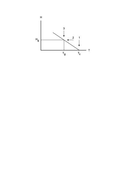
FIG. 1.: Schematic sketch of the $(H,T)$ phase diagram for the vortex–glass transition.

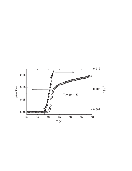
FIG. 2.: Temperature dependence of the resistivity $\rho$ and $(\ln\rho)^{-2}$ in zero field. The solid line is a fit to Eq. (29) providing an estimate for the Kosterlitz–Thouless transition temperature.

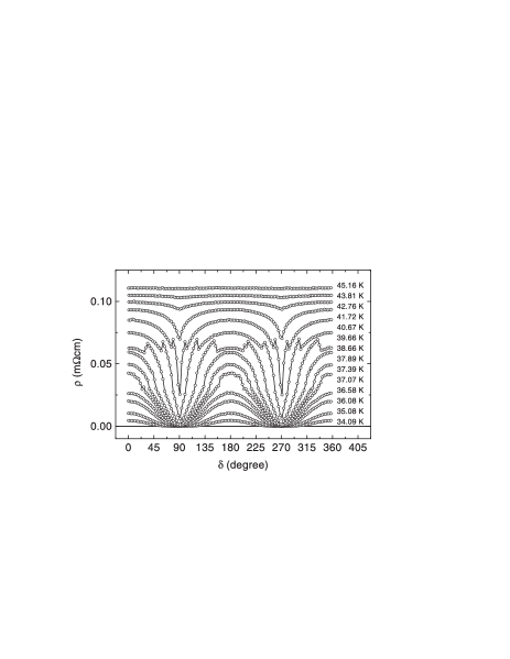
FIG. 3.: Angular dependence of the resistivity of a 120-Å-thick La_2-xSr_xCuO₄ film with $T_{c}(H=0)\approx 36.74$ K at various temperatures at $H=1$ T.

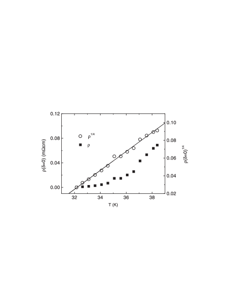
FIG. 4.: $\rho(\delta=0)$ versus $T$ and $\rho(\delta=0)^{1/4}$ versus $T$ at $H=1$ T, yielding the estimate $T_{g}\approx 29.7$ K.

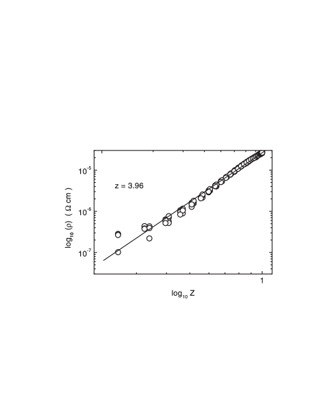
FIG. 5.: Log${}_{10}(\rho)$ versus $\log_{10}({\cal Z}(H,\delta))$ for $T=36.58$ K and $H=1$ T. The solid line corresponds to a linear fit yielding the estimate $z=3.96\pm 0.02$, using Eq. (43).

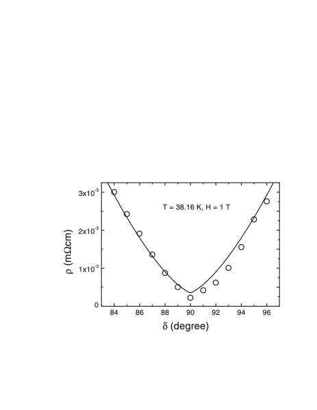
FIG. 6.: $\rho$ versus $\delta$ for $T=38.16$ K and $H=1$ T. The solid line is a guide to the eye to emphasize the characteristic 2D behavior (V-shape).

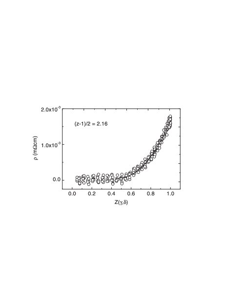
FIG. 7.: $\rho$ versus ${\cal Z}(\gamma,\delta)$ for $T=33.1$ K and $H=1$ T. The solid line is a fit to Eq. (47), yielding the parameters listed in Table I.

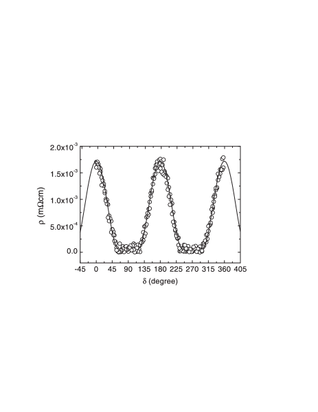
FIG. 8.: $\rho$ versus $\delta$ for $T=33.1$ K and $H=1$ T. The solid line corresponds to Eq. (47), with the parameters listed in Table I.

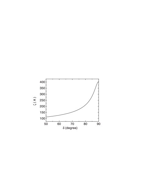
FIG. 9.: Contour plot of ${\cal Z}(\xi_{\|},\delta)=0.039$ [Eq. (48)] for $H=1$ T.