Numerical Replica Limit for the Density Correlation of the Random Dirac Fermion

Abstract

The zero mode wave function of a massless Dirac fermion in the presence of a random gauge field is studied. The density correlation function is calculated numerically and found to exhibit power law in the weak randomness with the disorder dependent exponent. It deviates from the power law and the disorder dependence becomes frozen in the strong randomness. A classical statistical system is employed through the replica trick to interpret the results and the direct evaluation of the replica limit is demonstrated numerically. The analytic expression of the correlation function and the free energy are also discussed with the replica symmetry breaking and the Liouville field theory.

72.15.Rn, 75.10.Nr

Although the scaling theory of localization for two-dimensional disordered systems generally predicts the absence of extended states, we have some examples of non-localized states in two dimensions which are marginally allowed to appear. Among them, systems with chiral symmetry such as the Anderson bond-disordered model [1], the random flux model [2, 3, 4] or the $\pi$-flux model with link disorders [5, 6] have attracted lots of attention. Density of states of the models have singularities at the zero energy and the corresponding wave functions exhibit multifractal behavior. Actually, one generally expects the existence of zero energy states for these models. Consider a Hamiltonian of the above models with chiral symmetry ${\cal H}=\sum_{<ij>}c_{i}^{\dagger}t_{ij}c_{j}+h.c.$ on a bipartite lattice $\Lambda$ which can be decomposed into two sublattices $\Lambda_{A}$ and $\Lambda_{B}$. After performing a unitary transformation (redefinition of indices), the Hamiltonian is expressed as

$${\cal H}=\pmatrix{\{c_{A}^{\dagger}\}&\{c_{B}^{\dagger}\}\cr}\pmatrix{{\bf 0}_{A}&{\cal D}_{AB}\cr{\cal D}_{AB}^{\dagger}&{\bf 0}_{B}\cr}\pmatrix{\{c_{A}\}\cr\{c_{B}\}\cr}.$$ (1)

The off-diagonal block structure of ${\cal H}$ implements the fact that hopping is restricted between the interpenetrating sublattices $\Lambda_{A}$ and $\Lambda_{B}$. The zero mode wave functions $\psi={}^{t}(\psi_{A},\psi_{B})$ satisfy the Schr$\ddot{o}$dinger equations

$${\cal D}_{AB}\psi_{B}=0,\hskip 28.45274pt{\cal D}^{\dagger}_{AB}\psi_{A}=0.$$ (2)

Let $N_{A,B}$ is the number of sites on $\Lambda_{A,B}$. For the cases where $N_{A}-N_{B}>0$ ( which can be realized, for example, by an appropriate boundary condition ), standard linear algebra tells us there always exist $(N_{A}-N_{B})$ independent zero energy solutions for Eq. (2) with vanishing $\psi_{B}$. In this expression, the notion of chiral symmetry is explicit. However, one needs to solve Eq. (2) numerically to go further.

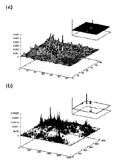
FIG. 1.: Typical probability densities $|\psi(x)|^{2}$ for $g=0.4$ on a (a) $64\times 64$ lattice and (b) $1024\times 1024$ lattice. Insets: $|\psi(x)|^{2}$ for $g=6.4$ for each system.

Now, let us concentrate our attention on cases where the low-lying physics is described by the Dirac fermions. Remarkably, in this situation, the explicit construction of zero energy wave functions is possible in a two-dimensional continuum space [7] [8]. Let us consider a Hamiltonian of the form $H={\bf\sigma}\cdot{\bf p}+{\bf\sigma}\cdot{\bf A}$ where $\sigma_{i=x,y}$ are the usual $2\times 2$ Pauli matrices and ${\bf A}$ is a random gauge field. The Schr$\ddot{o}$dinger (Dirac) equations for the zero modes are

$$(2\partial+i\bar{A})\psi_{-}=0,\hskip 28.45274pt(2\bar{\partial}+iA)\psi_{+}=0$$ (3)

where $\partial\equiv(\partial_{x}-i\partial_{y})/2$, $\bar{\partial}\equiv(\partial_{x}+i\partial_{y})/2$, $A\equiv A_{x}+iA_{y}$ and $\bar{A}\equiv A_{x}-iA_{y}$. This is a continuum analogue of Eq. (2). If we adopt the Coulomb gauge to express the vector potential ${\bf A}$ in terms of a scalar potential $\Phi$ as $A_{x}=\partial_{y}\Phi$, $A_{y}=-\partial_{x}\Phi$ and assume that the mean total flux piercing the system is zero, we can obtain the exact solution for any realization of disorders as $\psi_{\pm}({\bf x})=C_{\pm}e^{\mp\Phi({\bf x})}$. Further, let us assume the probability weight for each realization of $\Phi({\bf x})$ has the form $P[\Phi]\propto e^{-S}$ where $S[\Phi]=1/2g\int d^{2}x(\nabla\Phi({\bf x}))^{2}$ and $g$ is the disorder strength or, in the field theoretic language, the coupling constant, which is dimensionless in two dimensions.

From now on, we concentrate our attention only on $\psi_{+}$. For physical interest, it is necessary to consider normalized wave functions in a $L\times L$ box as $\psi({\bf x})=e^{-\Phi({\bf x})}/\sqrt{Z}$ with $Z=\int\frac{d^{2}{\bf x}}{a^{2}}e^{-2\Phi({\bf x})}$ where $a$ is a lattice constant. Here, we regularized the problem on a $N\times N$ periodic lattice although the original problem is formulated in a continuum space (where $L=Na$) . Correspondingly, we use the probability weight $S[\Phi]\propto 1/2g\sum_{<ij>}(\Phi_{i}-\Phi_{j})^{2}$ or, in the momentum space, $S[\Phi]\propto N^{2}/g\sum_{m}\widetilde{\Phi}_{m}\widetilde{\Phi}_{-m}\left(2-\sum_{\mu=1}^{2}\cos(ak_{m}^{\mu})\right)$ where $\widetilde{\Phi}_{m}\equiv N^{-2}\sum_{j}e^{-ik_{m}x_{j}}\Phi_{j}$ and the sum extends over the first Brillouin zone $m^{\mu}=-N/2+1\cdots N/2$ with $k_{m}^{\mu}=2\pi m^{\mu}/aN$ ($N$ is even for convenience.)[9]. Typical probability densities $|\psi(x)|^{2}$ calculated numerically are shown in Fig. 1, which remind us of multifractal states found at a localization-delocalization transition for several systems [10].

In fact, the multifractal property of this wave function has been revealed quantitatively by a close analogy to a generalized random energy model[11, 12]. As the disorder strength $g$ varied, the multifractal spectrum exhibits a sharp transition which is similar to the freezing phenomenon in spin glasses. Several other approaches such as the supersymmetry (SUSY) technique [13] , the connection to the Liouville field theory [14] , the renormalization group (RG)[15] or conformal field theory [16] have also been taken to support the transition.

Since the calculated probability densities (Fig. 1) are so spiky, the discretization procedure above may not be justified. In spite of this subtlety, we concentrate on this well defined discretized wave function to investigate universal properties.

In this letter, we evaluate the density correlation function

$$\left<\psi^{2}(1)\psi^{2}(2)\right>=\left<\frac{1}{Z^{2}}e^{-2\Phi({\bf x}_{1})}e^{-2\Phi({\bf x}_{2})}\right>$$ (4)

where $\left<\cdots\right>$ denotes the averaging with respect to the weight $P[\Phi]$. Here, the difficulties reside in the normalization factor $Z$ in the denominator since $Z$ itself is a random variable. The one of the simplest attempts to cope with it is the replica trick. We multiply the numerator by $Z^{n}$ and consider

$$\left<\psi^{2}(1)\psi^{2}(2)\right>_{n}\equiv$$ (5)

$$\int\frac{d^{2}\xi_{1}}{a^{2}}\cdots\frac{d^{2}\xi_{n-2}}{a^{2}}\left<e^{-2\left[\Phi({\bf x}_{1})+\Phi({\bf x}_{2})+\Phi({\bf\xi}_{1})+\cdots+\Phi({\bf\xi}_{n-2})\right]}\right>$$ (6)

which is expected to reduce to $\left<\psi^{2}(1)\psi^{2}(2)\right>$ by taking the replica limit $n\rightarrow 0$ (analytic continuation). We use this replica trick to interpret the direct numerical results and also try to take the replica limit by evaluating $\left<\psi^{2}(1)\psi^{2}(2)\right>_{n}$ numerically for several $n$ and extrapolating them to $n=0$. In addition, we utilize the evaluation of $\left<\psi^{2}(1)\psi^{2}(2)\right>_{n}$ together with the Liouville field theory to get the analytic expression of the correlation function for the weak disorder regime.

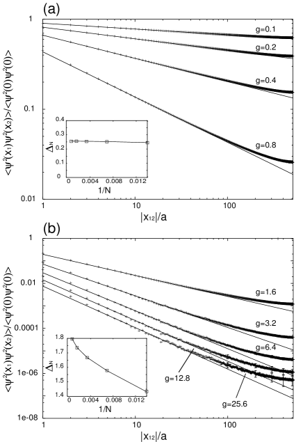
FIG. 2.: The numerically calculated density correlation for (a) the weak disorder regime and (b) the strong disorder regime on a $1024\times 1024$ lattice. For $g\leq 1.6$, the statistical error is smaller than the data point. For $g\geq 3.2$, the error bars are shown for every 100 points. Insets: The “exponent” $\Delta_{N}$ v.s. $1/N$ for (a) $g=0.4$ and (b) $g=6.4$. It is evaluated for $1\leq|x_{12}|/a\leq 10$ for each finite system.

First, let us present the direct numerical calculation of $\left<\psi^{2}(1)\psi^{2}(2)\right>$. In this problem, the probability weight itself is diagonal in the momentum space (see above), which allows us to carry out numerical simulations with a very large lattice up to $2048\times 2048$. Fig. 2 shows calculated $\left<\psi^{2}(1)\psi^{2}(2)\right>$ for various $g$ on a $1024\times 1024$ lattice. The quenched averaging is performed over $\sim 10^{5}$ different realization of disorders [17]. As is shown, the correlation function for the weak disorder exhibits power law behavior $\left<\psi^{2}(1)\psi^{2}(2)\right>\sim|x_{12}|^{-\Delta}$ for $1\lesssim|x_{12}|/a\ll N/2$ with its exponent $\Delta$ dependent linearly on $g$, $\Delta=2g/\pi$ (Fig. 3). It is consistent with the several analytic approaches [13]. As $g$ increases, however, the $g$ dependence of the correlation function becomes weaker and it deviates from the power law. To be more precise, there is a systematic deviation from the simple power law, that is, if we determine the “exponent” $\Delta_{N}$ on a finite $N$ system, it seems to diverge as $N$ increases ( see the insets of Fig. 2 ). It is clearly different from the behavior of $\Delta_{N}$ in the weak randomness where $\Delta_{N}$ seems to converge. In fact, as is shown in Fig. 1, the wave function becomes peaked on few sites as $g$ increases. However, it is different from the usual localized wave function which decays exponentially with its typical length scale characterized by the localization length. The above change of behavior in the correlation function is consistent with the transition from the weak to strong disorder found in the multifractal spectrum by the previous studies.

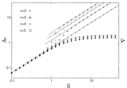
FIG. 3.: The “exponent” $\Delta_{N}$ of the two-point correlation function with respect to the disorder strength $g$ and its naive replica estimates $\Delta_{n=2,3,4,5}$ (log-log plot). The “exponent” is evaluated for $1\leq|x_{12}|/a\leq 10$ for $64\times 64$ ($\circ$), $256\times 256$ ($\Diamond$) and $1024\times 1024$ ($\bullet$) system. The statistical error is smaller than the symbol size. The analytic estimation Eq. (12) for $\Delta_{n}$ is represented by lines.

Next, let us try to interpret the above numerical results by the replica trick. After replicating $Z$, we can perform the averaging $\left<\cdots\right>$ in Eq. (5) and obtain

$$\left<\psi^{2}(1)\psi^{2}(2)\right>_{n} = \left<\delta(\xi_{k}-x_{1})\delta(\xi_{l}-x_{2})\right>^{cl}_{n}$$ (7)

with

$$\left<{\cal O}\right>^{cl}_{n} \equiv \mbox{Tr}\left[{\cal O}e^{-H_{n}}\right]/\mbox{Tr}\left[e^{-H_{n}}\right],$$ (8)

Tr $$\equiv \frac{1}{n!}\int\frac{d^{2}\xi_{1}}{a^{2}}\cdots\frac{d^{2}\xi_{n}}{a^{2}},$$ (9)

$$-H_{n} \equiv 4\sum_{k<l}^{n}{\cal G}(\xi_{k},\xi_{l}),$$ (10)

where $G(x_{i},x_{j})\equiv\left<\Phi(x_{i})\Phi(x_{j})\right>$ is the Green’s function and ${\cal G}(x_{i},x_{j})\equiv G(x_{i},x_{j})-G(0)\sim-g/2\pi\ln\left(|x_{ij}|/a\right)$. Here, we multiply some trivial factors which reduce to unity in the limit $n\rightarrow 0$. As is suggested in Eq. (7), $\left<\psi^{2}(1)\psi^{2}(2)\right>_{n}$ can be interpreted as the two body density of a classical statistical system consisting of a set of particles (replicas) interacting each other via the potential ${\cal G}(x_{i},x_{j})$[18]. These replica estimations are shown and directly compared to the numerical results (Fig. 4). In Fig. 4, $\left<\psi^{2}(1)\psi^{2}(2)\right>_{n}$ for various $n$ (the number of replicas) with fixed $g$ are obtained by calculating Eq. (7) numerically on a $64\times 64$ lattice. This rather small lattice size is due to the multiple integral in Eq. (7). Note that we do not have $\left<\psi^{2}(1)\psi^{2}(2)\right>_{n=1}$ as is inferred from Eq. (5). For $g=0.4$, the replica estimation seems to converge to the one calculated by the direct numerical simulations. For $g=6.4$, in contrast, it hardly seems to coincide to the exact one in the limit $n\rightarrow 0$. Moreover, it gives an unphysical result, i.e., a negative exponent, after taking the replica limit.

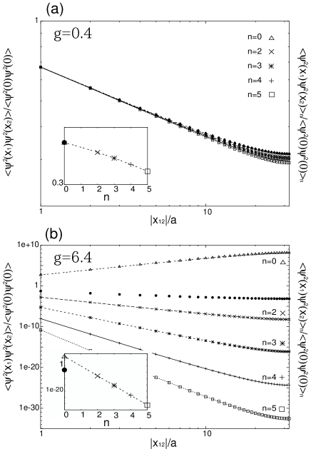
FIG. 4.: The numerically calculated density correlation ($\bullet$) and their replica estimates with the different number of replicas $n=2,3,4,5$ for (a) $g=0.4$ and (b) $g=6.4$ on a $64\times 64$ periodic lattice (log-log plot). The replica estimates are obtained by evaluating the multiple integral in Eq. (7) directly. $\left<\psi^{2}(x_{1})\psi^{2}(x_{2})\right>_{n=0}$ is obtained by extrapolating from $\left<\psi^{2}(x_{1})\psi^{2}(x_{2})\right>_{n=2,3,4,5}$. Insets: $\left<\psi^{2}(x_{1})\psi^{2}(x_{2})\right>_{n}$ v.s. $n$ at $|x_{12}|/a=20$ (semi-log plot).

This breakdown is closely related to the transition in the replica space. There are two distinct phases for this system. For small $g$, all configurations are equally favorable. As $g$ increases, however, the configurations where all replicas are close to each other come to have large weight. Thus, for sufficiently small $g$, it is enough to concentrate on only $\xi_{k}$ and $\xi_{l}$ in Eq. (7). The configuration of the other particles is smeared out in the ensemble average and irrelevant for $\left<\psi^{2}(1)\psi^{2}(2)\right>_{n}$. For large $g$, on the other hand, the main contributions in the ensemble average are from the configurations where all replicas except $\xi_{l}$ (or $\xi_{k}$) are at $x_{1}$ ( or $x_{2}$, respectively). Then, $\left<\psi^{2}(1)\psi^{2}(2)\right>_{n}$ is expected to behave as

$$\left<\psi^{2}(1)\psi^{2}(2)\right>_{n}\sim 1/|x_{12}|^{\Delta_{n}},$$ (11)

with

$$\Delta_{n}\sim\cases{2g/\pi&for small $g$\cr 2g(n-1)/\pi&for large $g$\cr}.$$ (12)

Numerically calculated $\Delta_{n}$ is shown in Fig. 3, which confirms the above estimation for small $n$ is reasonable. Taking the replica limit $n\rightarrow 0$, we obtain $\Delta_{n=0}=2g/\pi$ for small $g$ which is consistent with the results obtained by SUSY technique [13]. For the strong disorder regime, however, the exponent reduces to $-2g/\pi$ which is unphysical.

Does it mean the replica trick is a mere trick ? One of the possible scenarios is that the apparent breakdown is because we only take the small number of replicas into account. So, for large $n$, the $n$ dependence of $\Delta_{n}$ may deviate from Eq. (12) and give the correct answer in the replica limit [19]. Moreover, the replica symmetry breaking (RSB) solution which was proposed for the free energy[15] may be applicable also for the correlation function.

We also investigated other types of correlation functions such as $\left<\psi(1)\psi(2)\right>$ or $\left<\Phi(1)\psi^{2}(1)\Phi(2)\psi^{2}(2)\right>$ , the latter of which is of interest because it is related to the second derivative of the free energy $\left<\ln Z\right>/\ln\left(L/a\right)$ which shows the non-analyticity at $g=2\pi$. Their behaviors are qualitatively similar to that of $\left<\psi^{2}(1)\psi^{2}(2)\right>$ in that, for small $g$, these correlation functions become steeper and steeper as $g$ increases whose $g$ dependence are calculable by the replica trick. For large $g$, however, their $g$ dependencies are rather weak and the naive replica trick fails.

Another interesting approach is to utilize the formula $\frac{1}{Z^{N}}=\frac{1}{(N-1)!}\int_{0}^{\infty}d\mu e^{-\mu Z}\mu^{N-1}$ and express the correlation function as

$$\left<\psi^{2}(1)\psi^{2}(2)\right>=\int_{0}^{\infty}d\mu\mu\int{\cal D}\Phi e^{-2\Phi(x_{1})-2\Phi(x_{2})}e^{-S_{LFT}[\Phi]}$$ (13)

where $S_{LFT}=\int\frac{d^{2}\xi}{a^{2}}\left[1/2g\left(\nabla\Phi\right)^{2}+\mu e^{-2\Phi(\xi)}\right]$ [14]. This action resembles that of the Liouville field theory in two-dimensional quantum gravity. However, since it was pointed out that there are some subtleties about the field theoretic treatment of Eq. (13) [15], we evaluate it directly by using the replica estimates. We expand $e^{-\mu Z}$ to express $\left<\psi^{2}(1)\psi^{2}(2)\right>$ as the superposition of the replica estimates with a different number of replicas, i.e., the grand canonical ensemble

$$\left<\psi^{2}(1)\psi^{2}(2)\right>=2\int_{-\infty}^{\infty}d\widetilde{\mu}$$ (14)

$$\sum_{n=2}^{\infty}(-1)^{n}e^{-{\cal F}_{n}(\widetilde{\mu})}\left<\sum_{k\neq l}^{n}\delta(\xi_{k}-x_{1})\delta(\xi_{l}-x_{2})\right>_{n}^{cl}$$ (15)

where ${\cal F}_{n}(\widetilde{\mu})=-\ln\mbox{Tr}e^{-(H_{n}-\widetilde{\mu}n)}+2n^{2}G(0)$ and $\mu=e^{\widetilde{\mu}}$. Since for the weak disorder, the summand only trivially depends on $n$, we can easily sum up this suggestive expression and obtain the same result as the replica trick.

This method is applicable also for the free energy. We expand $\ln Z=\int_{0}^{\infty}\frac{d\mu}{\mu}\left(e^{-\mu}-e^{-\mu Z}\right)$ as

$$\left<\ln Z\right>=\int_{-\infty}^{\infty}d\widetilde{\mu}\left(e^{-e^{\widetilde{\mu}}}-1-\sum_{n=1}^{\infty}(-1)^{n}e^{-{\cal F}_{n}(\widetilde{\mu})}\right).$$ (16)

It is difficult to perform the summation for the strong disorder though we can obtain the correct answer for the weak disorder. However, if we simply employ the RSB estimate by Carpentier and Doussal[15], $e^{-{\cal F}_{n}}=n!^{-1}\left(L/a\right)^{(pg/\pi+2/p+\widetilde{\mu})n}$ where $p=1$ for the weak disorder and $\sqrt{2\pi/g}$ for the strong disorder, the summation reproduces the exact result both for the weak and strong disorder regime [19].

We thank Y. Morita for fruitful discussions. S.R. is grateful to T. Oka for useful comments. Y.H. was supported in part by a Grant-in-Aid from the Ministry of Education, Science, and Culture of Japan. The computation in this work has been partly done at the YITP Computing Facility and at the Supercomputing Center, ISSP, University of Tokyo.

REFERENCES

[1]
R. Gade,
Nucl. Phys. B 398, 499 (1993).
[2]
T. Sugiyama and N. Nagaosa,
Phys. Rev. Lett. 70, 1980 (1993).
[3]
Y. Avishai, Y. Hatsugai and M. Kohmoto,
Phys. Rev. B 47, 9561 (1993).
[4]
A. Furusaki,
Phys. Rev. Lett 82, 604 (1999)
and references therein.
[5]
Y. Hatsugai, X. -G. Wen and M. Kohmoto,
Phys. Rev. B 56, 1061 (1997).
[6]
Y. Morita and Y. Hatsugai,
Phys. Rev. Lett 79, 3728 (1997).
[7]
A. W. W. Ludwig, M. P. A. Fisher, R. Shankar and G. Grinstein,
Phys. Rev. B 80, 7526 (1994).
[8]
Y. Aharonov and A. Casher,
Phys. Rev. A 19, 2461 (1979)
[9]
We take
for any realization of disorders
since it just amounts
to a constant shift of which does not appear in .
[10]
See, for example,
B. Huckestein,
Rev. Mod. Phys. 67, 357 (1995)
and references therein.
[11]
C. Chamon, C. Mudry and X. -G. Wen,
Phys. Rev. Lett. 77, 4194 (1996).
[12]
H. E. Castillo, C. Chamon, E. Fradkin, P. M. Goldbart, C. Mudry,
Phys. Rev. B 56, 10668 (1997).
[13]
C. Mudry, C. Chamon and X. -G. Wen,
Nucl. Phys. B 466, 383 (1996).
[14]
I. I. Kogan, C. Mudry and A. M. Tsvelik,
Phys. Rev. Lett. 77, 707 (1996).
[15]
D. Carpentier and P. Le Doussal,
cond-mat/0003281.
[16]
V. Gurarie,
cond-mat/9907502.
[17]
Although there are no translational
and rotational invariance for a given realization of the disorder,
they are expected to be restored after taking the quenched averaging.
So, we numerically calculated
for a given realization of disorder
and took the averaging over disorder configurations.
[18]
Note that for
and by definition.
[19]
S. Ryu and Y. Hatsugai, in progress.
[20]
The RSB estimate for
is originally proposed for
and
it does not agree with the numerical
replica estimate for .
However, the success of the simple employment
of the RSB estimate
is mysterious and
seems to be related to the nature of the RSB.
Further exploration is interesting future issue.