Electrons on a sphere in disorder potential

Abstract

We investigate, both analytically and numerically, the behavior of the electron gas on a sphere in the presence of point-like impurities. We find a criterion when the disorder can be regarded as small one and the main effect is the broadening of rotational multiplets. In the latter regime the statistics of one impurity-induced band is studied numerically. The energy level spacing distribution function follows the law $P(s)\sim s\exp(-as^{b})$ with $1<b<2$. The number variance shows various possibilities, strongly dependent on the chosen model of disorder.

I introduction

A considerable amount of the theoretical interest has been devoted last years to the investigation of electronic properties of the nano-size objects possessing regular cylindrical and spherical shapes. While most of these studies were consecrated to the various properties of carbon nanotubes, the technological advances in production of spherical objects also require further theoretical understanding of peculiar quantum effects of electronic motion in such materials.

A well-known fullerene molecule, C₆₀, could be one of the examples, along with its further modification, so-called “onion” graphitic structures. [1] The spherical nano-size objects are also found in the studies of the nonlinear optical response in composite materials [2] and of simple metal clusters. [3] A rapidly evolving field of photonic-band-gap materials [4] provides yet another example of spheres of about 300 nm in diameter. In the latter case, one may find silica balls with semiconducting coating (coated opals) [5], or “inverse” opal structures, where the initial SiO₂ template is chemically removed and carbon spherical shells form three-dimensional fcc structure. [6]

In all these cases one can assume that the motion of itinerant electrons is confined within a spherical layer of a width small comparing to a radius. To a first approximation, one ignores the interaction effects and considers a situation of the electron gas. Theoretical efforts in this direction comprise an analysis of the behavior of such gas on a sphere in the uniform magnetic field and an evaluation of the electronic correlations without a field. It was shown particularly that if the field is small so that the magnetic length is larger than the radius, then one can expect the jumps in the magnetization and susceptibility of the sphere. [7, 8] An extension of this analysis for the ellipsoid of revolution has been undertaken recently. [9, 10] In stronger fields, when the magnetic length is smaller than radius, one finds a series of interesting effects described elsewhere. [11, 8]

The electronic correlation functions for the topology of the sphere exhibit, particularly, a peculiar coherence effect when the coherence length of electronic motion exceeds the radius of the sphere. [12] It turns out, that the amplitude of these functions is enhanced for the antipodal points on the sphere, where all partial waves of quantum motion come in phase.

The electron gas approximation, employed in these works, should be violated in experimental realizations of nanospheres. One of the reasons for this violation is the effects of electron-electron interaction, which were studied in [13].

Another source of possible inadequateness of the electron gas model is the explicit absence of rotational symmetry, inferred by the presence of impurities. Indeed, the experimental realization of the spherical layer, wherein the electrons are confined, might be far from the ideal shape. The inhomogeneities of various kind (impurities, fluctuations of layer’s width) should eventually destroy the effects, found theoretically for the idealized model. As a first crucial step here, one observes that the impurities necessarily raise the multiple degeneracy of the energy levels, found initially in a quantum rotator model of a free gas.

In this paper we consider the effects of potential impurity scattering in the electron gas on a sphere. We employ the model of point-like impurities, which is shown to be valid if the angular momentum of an electron does not exceed inverse angular range of the potential. Our results suggest that there is a definite range of parameters, where the electron gas approximation should be applicable. Particularly, this approximation is validated, when the radius of the sphere is smaller than the ratio $\sqrt{\nu}/\nu_{imp}$, with the areal densities of electrons and impurities, $\nu$ and $\nu_{imp}$, respectively. We show that in this case the degeneracy of the initially degenerate multiplet, close to Fermi energy, is lifted only partially. The unsplit states are superpositions of the initial spherical harmonics, and hence describe the electrons freely propagating along the sphere. As a result, one expects, that for sufficiently small disorder it is possible to discuss the coherence effects, induced by the spherical topology.

For the regime of weak disorder, we numerically investigated the splitting of on multiplet, caused by random impurities. We found that the statistics of the energy levels in this case is not identical, albeit close, to the predictions of the random matrix theory for the Gaussian orthogonal ensemble. Particularly we show that the energy level spacing distribution follows the law $P(s)\sim s\exp-s^{b}$, with $b\simeq 1.76$ in the limit of white-noise potential distribution. We discuss a possible reason for this deviation, related to the geometry of the problem.

A rest of the paper is organized as follows. We formulate the problem and treat the random potential perturbatively in Sec.  II. We identify here the region of parameters, where the perturbation theory fails. In Sec.  III we numerically investigate this region. The discussion and conclusions are presented in Sec.  IV.

II perturbative treatment of the impurity potential

A Green’s function

In the ideal situation the motion of an electron on the sphere is described by the quantum rotator model. The wave functions $\Psi$ are the spherical harmonics $Y_{lm}$ and the spectrum is simple :

$$\Psi(\theta,\phi)=r_{0}^{-1}Y_{lm}(\theta,\phi),\quad E_{l}=(2m_{e}r_{0}^{2})^{-1}l(l+1).$$ (1)

We normalize $\Psi(\theta,\phi)$ on the surface of the sphere $r_{0}^{2}\int|\Psi|^{2}\sin\theta d\theta d\phi=1$.

The main effect of the random impurity potential is the lifting of $(2l+1)-$fold degeneracy of each $l-$th energy level. Qualtitatively, one expects that at sufficiently small disorder these split levels form a subband nearly the initial position $E_{l}$, and the width of this subband does not exceed the separation between the adjacent levels $E_{l}$ and $E_{l\pm 1}$. This regime corresponds to the mean free path of the electron, $l_{mfp}$, larger than $r_{0}$. The coherence effects of the electronic motion should be still present in this case. [8, 12]

At larger disorder, the width of induced subband is more than $|E_{l}-E_{l\pm 1}|$. The different subbands overlap now and, as a result, one finds a constant density of states, typical for a planar two-dimensional electron gas. Having the relation $l_{mfp}<r_{0}$ in this case, one sees that the spherical surface is effectively decomposed onto the “patches” of size $l_{mfp}$, in which the electronic motion is essentially planar.

To find out the corresponding criterion for these two regimes, we use the Green function formalism. Treating disorder as perturbation, we write the self-consistent equation for the Green function. The spread of the split levels around the position of the initial multiplet is described by an imaginary part of the corresponding self-energy. This approach is very similar to one employed in the analysis of splitting of the lowest Landau level in two-dimensional electron gas (2DEG), [15, 14] and a reader can easily find parallels with our situation below.

The Green function is given by

$$G(\omega)=\sum_{lm}\frac{\Psi_{lm}^{\ast}(\theta^{\prime},\phi)\Psi_{lm}(\theta,0)}{\omega+\mu-E_{lm}},$$ (2)

For the free motion this expression simplifies

$$G^{0}(\omega)=(4\pi r_{0}^{2})^{-1}\sum_{l}\frac{(2l+1)P_{l}(\cos\Omega)}{\omega+\mu-E_{l}},$$ (3)

with the distance between two points on the sphere $\cos\Omega=\cos\theta\cos\theta^{\prime}+\sin\theta\sin\theta^{\prime}\cos\phi.$

The basic equation is

$$G(\Omega_{12})=G^{0}(\Omega_{12})+\int d{\bf r}_{3}d{\bf r}_{4}G^{0}(\Omega_{13})\Sigma(\Omega_{34})G(\Omega_{42})$$ (4)

where we write $\Omega_{12}$ for the angular distance between $\Omega_{1}$ and $\Omega_{2}$, etc. The integration over the surface of the sphere reads as $\int d{\bf r}=r_{0}^{2}\int d\Omega$.

Being averaged over disorder, the functions entering the above equation depend only on the distances between the corresponding points. Representing each function through its generalized Fourier coefficients,

$$F(\Omega)=r_{0}^{-2}\sum_{l}\frac{2l+1}{4\pi}F_{l}P_{l}(\Omega),$$ (5)

we have

$$G_{l}^{-1}=(G_{l}^{0})^{-1}-\Sigma_{l}$$ (6)

with $G_{l}^{0}=(\omega-E_{l})^{-1}$. We consider different contributions to $\Sigma_{l}$ below. But before doing that, we list some formulas applicable to the spherical geometry in the next subsection.

B some useful formulas

First we note that eq. (5) allows other representations, namely

$$F(\Omega_{12}) = r_{0}^{-2}\sum_{l}F_{l}A_{l}Y_{l0}(\Omega_{12}),$$ (7)

$$= r_{0}^{-2}\sum_{lm}F_{l}Y_{lm}^{\ast}(\Omega_{1})Y_{lm}(\Omega_{2}),$$ (8)

with the quantity

$$A_{l}\equiv\sqrt{(2l+1)/(4\pi)}.$$ (9)

The Green function (3) can be represented [8] through the Legendre function

$$G^{0}(\omega)=-\frac{m_{e}}{2\cos\pi\lambda}P_{-1/2+\lambda}(-\cos\Omega),$$ (10)

with $\lambda=\sqrt{2m_{e}r_{0}^{2}(\mu+\omega)+1/4}$. In subsequent consideration we are mostly interested in energies close to Fermi level, $\omega\ll\mu$. In this sense, we define the angular Fermi momentum, $L$, as $E_{L}\simeq\mu$, more precisely

$$\lambda \simeq L+1/2+(\omega-\Sigma_{l})/\Delta E$$ (11)

$$\Delta E = E_{L+1}-E_{L}=L/(m_{e}r_{0}^{2}).$$ (12)

For small angular distances $\Omega\ll\lambda^{-1}$ we have

$$G^{0}(\omega)\simeq\frac{m_{e}}{2\pi}\left[2\ln\left(\lambda\sin\frac{\Omega}{2}\right)+\gamma-\pi\tan\pi\lambda\right]$$ (13)

with the Euler constant $\gamma=0.577\ldots$. This expression is similar to the Green function for the 2DEG in the magnetic field $B$. Indeed, in the latter case we have for $r\ll l_{\ast}$ [16]

$$G^{0}(\omega)\simeq\frac{m_{e}}{2\pi}\left[2\ln\left(\frac{r}{l_{\ast}}\sqrt{\frac{\omega}{2\omega_{c}}}\right)-2\gamma-\pi\tan\pi\frac{\omega}{\omega_{c}}\right]$$ (14)

where the magnetic length $l_{\ast}=(eB)^{-1/2}$ and the cyclotron frequency $\omega_{c}=eB/m_{e}$.

For larger distances, $\lambda\sin\Omega\gtrsim 1$ we have approximately

$$G\simeq-\frac{m_{e}}{\sqrt{2\pi\lambda\sin\Omega}}\frac{\cos[\lambda(\pi-\Omega)-\pi/4]}{\cos\pi\lambda},$$ (15)

As was shown in [8], the existence of two oscillating exponents in (15) , $\exp\pm i\lambda\Omega_{12}$, indicates the interference of the partial waves on the sphere, one wave going along the shortest way between the the points $\Omega_{1}$ and $\Omega_{2}$, and another going along the longest way, turning around the sphere.

We discuss now a notion of point-like impurity on the sphere. Letting first the range of the potential to be zero, we write $u_{0}\delta({\bf r}-{\bf r}_{i})=u_{0}r_{0}^{-2}\delta(\Omega-\Omega_{i})\equiv u_{0}r_{0}^{-2}\delta(\cos\theta-\cos\theta_{i})\delta(\phi-\phi_{i})$ . Next we introduce the function describing the formfactor of impurity in the form $\delta_{a}({\Omega})=(2\pi a)^{-1}e^{(\cos\theta-1)/a}$, the limit $a\ll 1$ is assumed. The physical range of the potential is $r_{0}\sqrt{a}$. To exponential accuracy we have $\int d\Omega\delta_{a}({\Omega})=1$. Then, using the asymptotic (Macdonald) formula for the Legendre polynomials at small $\theta$, we calculate the auxiliary integral

$$\Delta_{l}\equiv A_{l}^{-1}\int d\Omega Y_{l0}(\Omega)\delta_{a}({\Omega})\simeq\exp\left(-a\frac{l(l+1)}{2}\right).$$ (16)

This equation shows that as long as considered moments $l<1/\sqrt{a}$, one can approximate the potential by delta function.

The impurity potential centered at the north pole reads as

$$u(\Omega)=u_{i}r_{0}^{-2}\delta_{a}({\Omega})=u_{0}r_{0}^{-2}\sum_{l}A_{l}\Delta_{l}Y_{l0}(\Omega)$$ (17)

and the potential centered at the point $\Omega_{i}$ is

$$u(\Omega-\Omega_{i})=u_{0}r_{0}^{-2}\sum_{lm}\Delta_{l}Y_{lm}^{\ast}(\Omega_{i})Y_{lm}(\Omega).$$ (18)

The averaging over the disorder $\overline{(\ldots)}$ is written as

$$\overline{u(\Omega_{1i})u(\Omega_{2i})} = \nu_{imp}r_{0}^{2}\int d\Omega_{i}u(\Omega_{1i})u(\Omega_{2i})$$ (19)

$$= \nu_{imp}u_{0}^{2}r_{0}^{-2}\sum_{l}\Delta_{l}^{2}A_{l}Y_{l0}(\Omega_{12})$$ (20)

$$= \nu_{imp}u_{0}^{2}r_{0}^{-2}\delta_{2a}({\Omega_{12}})$$ (21)

Here $\nu_{imp}=N_{imp}/(4\pi r_{0}^{2})$ is the impurity concentration and $N_{imp}$ is the total number of impurity centers.

Consider next more complicated objects, which are to be used below. If we have two functions, $f(\Omega)=\sum_{lm}f_{lm}A_{l}Y_{lm}(\Omega)$ and $g(\Omega)=\sum_{lm}g_{lm}A_{l}Y_{lm}(\Omega)$, then

$$f(\Omega)g(\Omega) = \sum_{l_{i},m_{j}}(f_{l_{1}m_{1}}g_{l_{2}m_{2}}V^{l_{3}m_{3}}_{l_{1}m_{1}l_{2}m_{2}})A_{l_{3}}Y_{l_{3}m_{3}}(\Omega)$$ (22)

$$V^{l_{3}m_{3}}_{l_{1}m_{1}l_{2}m_{2}} = A_{l_{1}}^{2}A_{l_{2}}^{2}A_{l_{3}}^{-2}C^{l_{3}0}_{l_{1}0l_{2}0}C^{l_{3}m_{3}}_{l_{1}m_{1}l_{2}m_{2}}$$ (23)

with the Clebsch-Gordan coefficients $C^{lm}_{l_{1}m_{1}l_{2}m_{2}}$. [17]

Particularly, when $f(\Omega)=\delta_{a}({\Omega})$ and $g(\Omega)$ can be approximated by a constant $\tilde{g}$ at small $\Omega\leq\sqrt{a}$, we have $(f\cdot g)_{lm}=\tilde{g}\Delta_{l}\delta_{m0}$.

C perturbation theory

We use the model of point-like impurities randomly distributed on the sphere. The amplitudes $u_{0}$ of the impurity potential are chosen to be equal. The overall potential is

$$U(\Omega)=u_{0}r_{0}^{-2}\sum_{lm}\Delta_{l}Y_{lm}^{\ast}(\Omega)\sum_{i=1}^{N_{imp}}Y_{lm}(\Omega_{i})$$ (24)

As usual, the average of this potential gives a constant, which is incorporated into the chemical potential and is discarded below. First nontrivial diagrams in the perturbation series in $u_{0}$ are shown in Fig. 1.

FIG. 1.: First diagrams describing impurity scattering

In the self-consistent Born approximation, we find for the self-energy in the second order of $U$, Fig. 1a

$$\Sigma^{(a)}(\Omega)=\nu_{imp}u_{0}^{2}r_{0}^{-2}\delta_{2a}(\Omega)G(\Omega)$$ (25)

so that $\Sigma_{l}^{(a)}$ is independent of $l$ (as long as $\Delta_{l}\simeq 1$)

$$\Sigma_{l}^{(a)}=\nu_{imp}u_{0}^{2}G(\Omega\sim\sqrt{a})$$ (26)

The last line is obtained upon an assumption $L\sqrt{a}<1$, when the argument of the logarithm in (13) is small. Recalling that $L\leftrightarrow k_{F}r_{0}$, the latter condition means that the range of the impurity potential does not exceed $k_{F}^{-1}$ in real space.

Letting $\omega=0$ and introducing the quantity

$$z=\pi\Sigma_{l}/\Delta E$$

we find the self-consistency equation in this order of $U$ :

$$z \simeq X\tilde{u}^{2}\left(\frac{2}{\pi}\ln(L\sqrt{a})-\cot z\right),$$ (27)

with

$$X=N_{imp}/(2L+1),$$ (28)

and the dimensionless scattering amplitude

$$\tilde{u}=u_{0}m_{e}/2.$$ (29)

In the following we adopt the picture of the weak scattering, $\tilde{u}\ll 1$.

The real part of $\Sigma_{l}$ in (27) redefines the chemical potential and may be ignored. The imaginary part of $\Sigma_{l}$ describes the width of the impurity-induced band, arising instead of degenerate multiplet $L$ :

$$z = X\tilde{u}^{2}\left(\frac{2}{\pi}\ln(L\sqrt{a})-i\right),\quad X\tilde{u}^{2}\gtrsim 1$$ (30)

$$= -i\sqrt{X}\tilde{u},\quad X\tilde{u}^{2}\lesssim 1$$ (31)

As we discussed above, the second regime is of our main interest. It corresponds to the case when the $\cot z$ dominates over the logarithm in (27), which in turn means the possibility to ignore the transitions between the levels with different $l$. The scattering in this case is between the states with different $m$ within one multiplet $l$.

The next diagram, Fig. 1b, is wrtten in the form

$$\Sigma^{(b)}(\Omega)\simeq\nu_{imp}u_{0}^{3}r_{0}^{-2}\delta_{a}(\Omega)G^{2}(\Omega).$$ (32)

Or, in the previous notation

$$\frac{\pi\Sigma^{(b)}_{l}}{\Delta E}\simeq X\tilde{u}^{3}\left(\frac{2}{\pi}\ln(L\sqrt{a})-\cot z\right)^{2}.$$ (33)

In order to find the relative importance of this correction, we put the former estimate, $\Sigma^{a}$, into the energy argument of the Green function, $\lambda\simeq l+1/2-\Sigma_{l}^{a}/\Delta E$. Then we find

$${\Sigma^{b}_{l}}/{\Sigma^{a}_{l}} \sim \tilde{u},\quad X\tilde{u}^{2}\gtrsim 1,$$ (34)

$$\sim X^{-1/2},\quad X\tilde{u}^{2}\lesssim 1.$$ (35)

Evidently, the correction $\Sigma^{b}$ can be neglected at large $X$ and dominates at $X<1$. We discuss this feature in more detail below.

The next diagram is shown in the Fig.  1c

$$\Sigma^{c}(\Omega)=\nu_{imp}^{2}u_{0}^{4}G(\Omega)^{3}$$ (36)

The Fourier component $\Sigma^{c}_{l}$ behaves differently in the two above cases $z>1$ and $z<1$.

In the case $z\ll 1$ the Green function can be approximated by the expression (3). Near the level $E_{L}$ we have

$$G \simeq (4\pi r_{0}^{2})^{-1}\frac{(2L+1)P_{L}(\cos\Omega)}{\omega+\mu-E_{L}-\Sigma_{L}},$$ (37)

$$\simeq -\frac{m_{e}}{z}\frac{\cos[(L+1/2)\Omega-\pi/4]}{\sqrt{2\pi L\sin\Omega}},\quad L\sin\Omega\gtrsim 1$$ (38)

where we have put $\omega=0$ in the last line. Using (37) and (38), one finds for $\Sigma^{c}_{l}$ the following expressions, respectively,

$$\Sigma^{c}_{l} \simeq -\nu_{imp}^{2}u_{0}^{4}r_{0}^{2}\left(\frac{\pi m_{e}}{zLr}\right)^{3}\sum_{l_{1}}V^{L0}_{l_{1}0l0}V^{l_{1}0}_{l0l0},$$ (39)

$$\simeq -\frac{3}{2}\nu_{imp}^{2}u_{0}^{4}A_{l}^{-1}\left(\frac{m_{e}}{2\pi zA_{L}}\right)^{3}\ln\left|\frac{L}{L-l}\right|.,$$ (40)

$$\simeq -\Delta E\frac{3X^{2}\tilde{u}^{4}}{\pi^{3}\sqrt{lL}z^{3}}\ln\left|\frac{L}{L-l}\right|..$$ (41)

Note that the expression (39) tells us that : i) $l$ and $L$ are even (odd) simultaneously, i.e. $(L+l)=0{\rm mod}2$, and ii) $\Sigma^{c}_{l}=0$ at $l>3L$. The Eq. (39) is not convenient and one can use an approximate expression (41). In the considered case (31) we estimate at $l=L$ :

$${\Sigma^{c}_{L}}/{\Sigma^{a}_{L}} \sim L^{-1}\ln L\ll 1$$ (42)

Therefore this correction is smaller than the previous one.

The case $Im\,z>1$ corresponds to the mean free path of the electron smaller than $r_{0}$. In this case the Green function (15) exhibits the presence of only one wave, with the shorter path. One has from (15) at $Im\lambda\gtrsim 1$ :

$$G\simeq-\frac{m_{e}}{\sqrt{2\pi\lambda\Omega}}\exp\left[i\lambda\Omega+i\frac{\pi}{4}\right],$$ (43)

As a result we have

$$\Sigma^{c}_{l} \simeq \Delta E\frac{X^{2}\tilde{u}^{4}}{L}f\left(\frac{l+1/2}{3\lambda}\right)$$ (44)

$$f(x) = \frac{(2/\pi)^{3}}{\sqrt{6(1+x)}}K\left[\frac{2x}{1+x}\right].$$ (45)

with the complete elliptic integral $K(x)$ and $\lambda\simeq L+1/2+z/\pi$. A comparative importance of this contribution is

$${\Sigma^{c}_{L}}/{\Sigma^{a}_{L}} \sim X\tilde{u}^{2}/L$$ (46)

and may be significant in the considered case $X\tilde{u}^{2}>1$.

One can evaluate also a sixth-order correction, shown in the Fig. 2, which is the next non-trivial term. In case of our interest, $X\tilde{u}^{2}\lesssim 1$, the contribution of this diagram, $\Sigma^{d}$, is estimated as follows.

$$\Sigma^{d}_{l=L} \simeq \Delta E\frac{X^{3}\tilde{u}^{6}}{z^{5}}\frac{4}{\pi^{3}L}$$ (47)

so that the relative importance of this diagram is again small :

$${\Sigma^{d}_{L}}/{\Sigma^{a}_{L}}\sim 1/L$$ (48)

FIG. 2.: A sixth-order diagram with maximally crossed impurity lines

One can further argue that the weak localization corrections do not contribute much at $X\tilde{u}^{2}<1$. Indeed, in this case of our interest below, when the mean free path is larger than the radius, we are essentially in the ballistic regime, hence one does not find a typical enhancement in the cooperon series. As a result, the arguments elucidating the role of the spherical topology in the diffusive regime [18] cannot be fully applied to our case.

On the other hand, let us consider a diagram which describes four scattering events on the same impurity. This is the next diagram in a sequence, formed by Figs. 1a, 1b. It can be easily shown, that in the regime (31) this diagram is estimated as $\Sigma^{a}_{L}/X$, being thus large at $X<1$. This latter sequence of diagrams contributes to the S-matrix for one impurity. The formal divergence in this sequence at $X<1$ indicates a singularity in the S-matrix. In the following section we show, that this singularity corresponds to the incomplete raising of degeneracy in $L-$th multiplet.

Note that the quantities $L$, $X$ and $(\Delta E)^{-1}$ scale as $r_{0}$ so that in the limit of large sphere the regime (31) does not occur and we are left with eqs. (30), (34), (46). It is worth to represent the quantity $X$ in the form

$$X=\frac{\nu_{imp}}{\sqrt{\nu/\pi}}r_{0},$$ (49)

then we see that the criterion $X<1$ means $r_{0}\lesssim\sqrt{\nu}/\nu_{imp}$. For the semiconducting situation, adopting a simple estimate $\nu\sim\nu_{imp}\sim 10^{10}\,$cm^-2, we get for this regime $r_{0}\lesssim 100\,$nm, the latter value comparable to the size of opal balls.

Concluding this section, we observe that at sufficiently small disorder, $X\tilde{u}^{2}<1$, the impurity-induced bands, referring to different multiplets, do not overlap. This regime corresponds to the scattering mostly within one multiplet. At small $X$ one meets a singularity in S-matrix of scattering for one impurity. We consider it to some detail in the next section.

III scattering within a multiplet

In this section we restrict ourselves by the analysis of the scattering within a multiplet, characterized by the quantum number $L$. Initially this multiplet is $(2L+1)-$fold degenerate. The impurities lower the rotational symmetry and lift the degeneracy. The transitions between the multiplets with different $L$ are neglected. The matrix elements of the Hamiltonian are the projection of the impurity $\delta-$functions onto the multiplet, and we have

$${\cal H}_{m,n} = \sum_{i=1}^{N_{imp}}u_{i}r_{0}^{-2}Y_{Lm}^{\ast}(\Omega_{i})Y_{Ln}(\Omega_{i})$$ (50)

In this section, in order to obtain a wider picture, we allow a variation of $u_{i}$. Specifically, we numerically consider three possibilities  : i) the former case, all $u_{i}=u_{0}$, ii) $u_{i}=\pm u_{0}$ and $\overline{u_{i}}=0$, and iii) $u_{i}$ is a normally distributed (ND) variable with variation $u_{0}$, $\overline{\exp(iku_{j})}=\exp(-k^{2}u_{0}^{2}/2)$.

Simple estimates show that the average off-diagonal matrix element of $\cal H$ scales in the limit of large $N_{imp}$ as

$$\overline{|{\cal H}_{m,n}|^{2}}\sim u_{0}^{2}r_{0}^{-4}N_{imp}$$ (51)

In this limit one may also regard different ${\cal H}_{m,n}$ to be almost statistically independent quantities. Due to the known property of large random matrices, it follows then that the width of the impurity-induced band will be of order of $u_{0}r_{0}^{-2}\sqrt{N_{imp}L}$. This estimate corresponds to the above one, eq. (31), and is validated by the numerical calculations. At the same time, some features of our problem prevent us from an identification of ${\cal H}$ with one of the classes of random matrices. Hence the usual expectations from the random matrix theory might not be fully applicable to our case. We discuss these points in the next subsections.

A Lifshits’s theorem

There exists a particular property, satisfied when the degeneracy $(2L+1)$ is larger than the number of impurity centers, $N_{imp}$. In this case at least $2L+1-N_{imp}$ levels remain degenerate for any choice of $u_{i},\Omega_{i}$. This statement is a general one for the projective perturbations and dates back to the work by Lifshits [19]. It is known particularly for the impurity scattering of the electrons in a magnetic field.[15, 14] For a sphere, this statement can be proved as follows.

Let us write $Y_{Lm}(\Omega_{i})\equiv\langle i|m\rangle$ and introduce a scalar product for two points on the sphere as

$$\langle i|j\rangle = \sum_{m}Y_{Lm}^{\ast}(\Omega_{j})Y_{Lm}(\Omega_{i})=\frac{2L+1}{4\pi}P_{L}(\cos\Omega_{ij})$$ (52)

We introduce also a real-valued matrix ${\cal M}$ with elements

$${\cal M}_{ij}=u_{i}r_{0}^{-2}\langle i|j\rangle.$$ (53)

Then ${\rm Tr}{\cal H}=\sum_{im}u_{i}r_{0}^{-2}\langle m|i\rangle\langle i|m\rangle={\rm Tr}{\cal M}$, and ${\rm Tr}{\cal H}^{2}=\sum_{ijmn}u_{i}u_{j}r_{0}^{-4}\langle n|i\rangle\langle i|m\rangle\langle m|j\rangle\langle j|n\rangle={\rm Tr}{\cal M}^{2}$, and generally

$${\rm Tr}{\cal H}^{k}={\rm Tr}{\cal M}^{k}.$$ (54)

After this observation it is straightforward to show that

$$det(E-{\cal H}) = \exp\left[(2L+1)\ln E+{\rm Tr}\ln(1-{\cal H}/E)\right]$$ (55)

$$= \exp\left[(2L+1)\ln E+{\rm Tr}\ln(1-{\cal M}/E)\right]$$ (56)

$$= E^{2L+1-N_{imp}}det(E-{\cal M}).$$ (57)

In the last line the pole in $E$ at $2L+1<N_{imp}$ is compensated by the necessary degeneracy of the matrix $\cal M$ in this case.

Therefore a singularity in the S-matrix of perturbation theory is identified with the incomplete raising of degeneracy.

Another specific feature of our problem is the following. We see that non-zero eigenvalues of (50) coincide with those of (53) which is a real symmetric matrix (for $u_{i}=u_{0}$) with a randomness in its elements. Then one should seemingly classify $\cal M$ to Gaussian orthogonal ensemble (GOE). However, the elements of $\cal M$ are not statistically independent. Indeed, it can be easily shown, that averaging over positions of impurities gives

$\displaystyle\overline{{\cal M}_{ij}^{2}}=\frac{(2L+1)u_{0}^{2}}{(4\pi)^{2}r_{0}^{4}}\equiv Q^{2},$

while, e.g., the triple combination with the cyclic sequence of indices yields

$\displaystyle\overline{{\cal M}_{ij}{\cal M}_{jk}{\cal M}_{ki}}=\frac{Q^{3}}{\sqrt{2L+1}}\neq 0.$

This fact of nonvanishing long-range correlations makes our problem distinct from the usually considered ones. Being small, these correlations however should cause only minor deviations from the GOE predictions.

For the case, when the amplitudes $u_{i}$ are sign-reversal, $\cal M$ is not symmetric and one expects larger deviations from the known picture.

B numerical results

We performed the numerical diagonalization of the matrices of the form (50), with the positions $\Omega_{i}$ randomly distributed on the sphere and the amplitudes $u_{i}$ chosen according to one of the above ensembles. The calculations were done with the use of standard EISPACK routines for $10,000$ random realizations of $\Omega_{i},u_{i}$ for each $L,N_{imp}$.

For given $L,N_{imp}$, we determine the density of states $\rho(E)$ (DOS), averaging over the realizations. The density is normalized as $\int_{-\infty}^{\infty}\rho(E)\,dE=2L+1$ . Some typical curves for DOS are shown in the Fig. 3. We observe following qualitative features :

i) For identical impurities, $u_{i}=u_{0}$, we have a smooth asymmetric DOS at $X>1$, when the degeneracy is removed. At the point $X=1$, DOS exhibits a mild singularity, roughly of the law $\ln^{2}E$. When $X<1$, a part of the multiplet is unsplit, and the split-off states are separated from the position of this $\delta-$function. For a convenience of presentation of Fig. 3a, we shifted the energies by $\mbox{Tr}{\cal H}/(2L+1)=\nu_{imp}u_{0}$. As a result, the DOS is centered for each $X$, i.e. $\int_{-\infty}^{\infty}E\,\rho(E)\,dE=0$.

ii) For the “dichotomic” impurities, $u_{i}=\pm u_{0}$, $\overline{u_{i}}=0$, the DOS is symmetric, showing the same features as in the case (i).

iii) For the case of the normally distributed $u_{i}$, the properties of DOS are similar to the case (ii), except for the region $X<1$. In this latter region, $\rho(E)$ shows a mild singularity at $E=0$, accompanied by $\delta-$function contribution of unsplit states.

In order to test the accuracy of calculations, we fixed the window for the expected $N_{0}=2L+1-N_{imp}$ unsplit states to the size $10^{-6}$ of estimated band-width. The average number of energy levels, found in this window was $N_{0}+\delta N$ with $\delta N\ll 1$. In the worst case of ND amplitudes $u_{i}$ and $X<1$ we had $\delta N\lesssim 10^{-3}$. The small values of $\delta N$ allowed us to separate the smooth contribution from the $\delta-$core.

As a next step, we unfolded the spectrum, $\{E_{i}\}\to\{\varepsilon_{i}\}$ by defining $\varepsilon_{i}=\int_{-\infty}^{E_{i}}\rho(E)\,dE$. A certain subtlety in this procedure should be described here. If the degeneracy of the multiplet is completely removed, then the average spacing $s_{i}\equiv\varepsilon_{i+1}-\varepsilon_{i}$ between the nearest neighboring $\varepsilon_{i}$ is $\overline{s_{i}}=1$. We examine also the statistics of the spectrum for the partially degenerate level when the DOS contains a smooth part and a singular contribution, $\rho(E)=\rho_{smooth}(E)+N_{0}\delta(E)$. To describe this case, we exclude the states in the $\delta-$core from our consideration and write for the split levels $\varepsilon_{i}=\int_{-\infty}^{E_{i}}\rho_{smooth}(E)\,dE$. Obviously, upon doing this, we have again $\overline{(\varepsilon_{i+1}-\varepsilon_{i})}=1$, now with $i=1,\ldots,N_{imp}-1$.

We studied the energy level spacing distribution function $P(s)$ with the use of the unfolded spectrum. We remind, that usually in analyzing the spectrum of random ensembles, one finds either the Wigner-Dyson (WD) law, $P(s)\sim s\exp(-s^{2})$, established for the GOE ensemble, or the Poissonian law, $P(s)\sim e^{-s}$. Besides, it was shown that in the vicinity of the metal-insulator Anderson transition (MIT) an intermediate distribution may take place, which interpolates between the WD and Poissonian dependence. [20] Particularly, one observes a “semi-Poisson” distribution, $P(s)=4se^{-2s}$ in three dimensions (D) at MIT. [21] Similar intermediate $P(s)$ occur also in the studies of the statistics of the lowest Landau level in the presence of disorder [22] and in some other models. [23]

It turned out, that our data are well described (with some predictable exclusions, discussed below) by the following formula

$$P(s)=cs\,\exp(-as^{b}).$$ (58)

Since the conditions $\int P(s)ds=\int s\,P(s)ds=1$ uniquely determine the parameters $a,c$ in the form

$$a = \left({\Gamma[3/b]}/{\Gamma[2/b]}\right)^{b},$$ (59)

$$c = b\,\Gamma[3/b]^{2}\,\Gamma[2/b]^{-3},$$ (60)

the eq. (58) depends, in fact, only on $b$. This parameter was determined by fitting the numerically obtained curves both for $P(s)$ and $\ln P(s)$. Remarkably, in those cases, when a good visual agreement of the data with a fitting curve was achieved, the values of $b$, determined both ways, essentially coincided. Some of the results are shown in Fig. 4, 5, 6, 7.

The values of $b$ are summarized in the Table I. In cases of good visual agreement, the corresponding error in $b$ was $\pm 0.01$, estimated from the different fitting procedures used. From this table, we see that the values of $b$ in the investigated range of $L$, $N_{imp}$ depend only on the ratio of these quantities. The obtained $b$s are essentially the same in each of two domains $X>1$ and $X<1$, with somewhat lower $b$s at $X<1$. The worse agreement with the fit was obtained in the cases, when the regular part of DOS, $\rho_{smooth}(E)$ showed a mild singularity, Fig.  3. In these cases we checked the procedure of unfolding the spectrum, which included the cubic spline interpolation. The range of $E$ was divided, so that the position of singularity corresponded to a free boundary of a spline. The resulting spline curve fitted $\rho_{smooth}$ well, showing no oscillations , however, it did not improve the quality of the fit of $P(s)$ by eq. (58). Particularly, the tail of $P(s)$ in these cases showed roughly exponential decay $\ln P(s)\sim-s$ at larger $s$ and a small non-vanishing value of $P(s=0)$, which can be expected for the systems with a localization of the states. The results of the fit of this tail by the exponential law for the normally distributed $u_{i}$ are shown in Fig.  II. It is seen here, that $P(s)$ at large $s$ decreases faster with the increase of disorder $X$.

The linear tail in $\ln P(s)$ at large $s$ for the singular DOS can be, in principle, expected. One can argue that in this case the unfolding procedure itself is not particularly useful. Indeed, this procedure assumes that different parts of the spectrum can be treated on equal grounds. This assertion can be tolerated for unsingular DOS, while the presence of a singularity in $\rho_{smooth}$ explicitly breaks the premise for the unfolding, $E_{i}\to\varepsilon_{i}$. As a result, one anticipates that the part of the spectrum at the center of the band shows the intermediate statistics, which is different from the Poissonian one, stemming from the localized states at the tails of the band (see, e.g., Ref. [22]).

Note, that the considered cases of dichotomic and ND amplitudes lead to the same value of $b=1.76\pm 0.02$ at $X\gtrsim 3$. By analogy with the integer quantum Hall effect (IQHE) [24] one can argue that the limit of large $X$ corresponds to the white noise distribution of impurity potential ( $X$ is associated with the number of impurities per one flux quantum). Our findings suggest that $b\neq 2$ in this limit.

Next, we performed the analysis of the number variance,

$$\Sigma^{2}(\varepsilon)=\overline{N^{2}(\varepsilon)}-\left(\overline{N(\varepsilon)}\right)^{2},$$ (61)

which measures the fluctuation of the number of levels $N(\varepsilon)$ in a band of unfolded spectrum of width $\varepsilon$. The number variance is generally believed to be more sensitive than $P(s)$ to the change of ensemble statistics. One has $\Sigma^{2}(\varepsilon)=\varepsilon$ for the Poisson sequence, while GOE prediction is $\Sigma^{2}(\varepsilon)\sim 2\pi^{-2}\ln\varepsilon$ at large $\varepsilon$. For the intermediate statistics at MIT, earlier theoretical arguments [25, 26] suggested that $\Sigma^{2}(\varepsilon)\propto\varepsilon^{2-b}$, later it was agreed that $\Sigma^{2}(\varepsilon)\sim\chi\varepsilon$ with $\chi<1$. [27, 28, 29]

Since we deal with finite size matrices, the range of $\varepsilon$ is restricted from above by $(2L+1)$. Actually the finite-size effects are felt at $\varepsilon\sim 0.4(2L+1)$, where one finds a maximum of $\Sigma^{2}$. The behavior of the number variance at lower $\varepsilon$ is shown in Fig. 8.

From this figure one sees that in the case (i) of identical impurities $\Sigma^{2}$ follows the GOE prediction except for the value $X=1$. In cases (ii) and (iii), when $u_{i}$ are allowed to vary, the dependence $\Sigma^{2}(\varepsilon)$ goes visibly above the GOE law. One notices that in the case (iii) of ND $u_{i}$ the obtained $\Sigma^{2}$ is considerably higher than in the case (ii) of dichotomic amplitudes. The highest curve for the number variance is obtained again at $X=1$, both for the case (ii) and (iii).

The pronounced variation of $\Sigma^{2}$ with $X$ in two latter cases should be contrasted with our results for $P(s)$, Table I. Indeed, we see that the the curves for $\Sigma^{2}$ may almost coincide for different $b$’s (at $X<1$ and $X>1$), while they may be notably different for almost identical $b$’s. Particularly, one finds almost linear dependence at $\varepsilon\gtrsim 3$ , $\Sigma^{2}(\varepsilon)\simeq\chi\varepsilon+const$ with $\chi<1$. The slopes $\chi$ vary in the range $0.06\div 0.14$ and $0.1\div 0.4$ for the dichotomic and ND amplitudes, respectively.

Making this observation we try to compare our system with the problems of metal-insulator Anderson transition and of impurity-split lowest Landau level. We mentioned the earlier theoretical expectation $\Sigma^{2}(\varepsilon)\propto\varepsilon^{2-b}$ above. This possibility, numerically validated for the 3D MIT [30] is apparently not favored by our data. Other studies support the viewpoint that $\Sigma^{2}(\varepsilon)\propto\chi N$ with the level compressibility $\chi<1$ (see [31] for a review). A relation $2\chi=1-D_{2}/d$ connects [29, 32] the quantity $\chi$ with the multifractal exponent $D_{2}$, characterizing the spatial extent of the wave functions in the flat geometry of $d$ dimensions, $\int d{\bf r}\,|\psi|^{4}\propto V^{-D_{2}/d}$ with $V$ a volume of the system. For the IQHE various authors provided the values $D_{2}=1.4\div 1.6$ and $\chi=0.1\div 0.15$. [33, 34, 35]

The values of $\chi$ extracted from our data are roughly consistent with these results. A pronounced dependence of $\chi$ on $X$, however, requires further understanding. We suggest here that
i) either our results obtained for $\varepsilon\leq 15$ do not describe the true asymptote of $\Sigma^{2}$, (cf. [30, 21])
ii) or the multifractal exponent $D_{2}$ varies with $X$.

It would be interesting to check the last possibility by investigating the spatial character of the wave functions in our model. This work is however beyond the scope of the present study.

IV Discussion and conclusions

We considered the electron gas on the sphere, moving in the potential field of point-like scatterers. Without a disorder, one observes a series of effects, associated with the coherent motion of the electrons in the spherical geometry. The high symmetry of a problem leads to the large degeneracy of energy spectrum in the ideal case. The disorder removes the rotational symmetry, prompting one to expect the disappearance of the coherence effects.

Our consideration shows that there exist a definite range of disorder parameters, where the sphere remains sphere at least partly. Particularly we demonstrate that the phenomenon of incomplete raising of degeneracy may take place for sufficiently small radii. In the case of relatively small disorder the main effect is the splitting of the rotational multiplet, while the transitions between the different multiplets can be ignored. Numerically investigating this latter case, we studied the energy level statistics in the impurity-induced band. We found that the energy spacing distribution function follows a modified Wigner-Dyson law, $P(s)\sim s\exp(-s^{b})$ with $b\simeq 1.76$ in the white noise limit. Our data suggest that the parameter $b$ does not determine the behavior of the energy levels’ number variance $\Sigma^{2}$. The latter quantity reveals various possibilities for almost the same values of $b$, depending strongly on the chosen model of disorder.

TABLE I.: The values of the best fit to $P(s)$ by the formula $P(s)=cs\,\exp(-as^{b})$. Parameters $a,c$ depend on $b$ as described in text.

$(2L+1)$	$N_{imp}$	$X$	$b(u_{i}=1)$	$b(u_{i}=\pm 1)$	$b(u_{i}=ND)$
61	300	4.92	1.88	1.74	1.78
41	200	4.88	1.89	1.76	1.76
41	120	2.93	1.89	1.75	1.75
41	50	1.22	1.86	1.73	1.62 a
61	61	1	1.64	1.68	1.34a
61	50	0.82	1.80	1.68	1.45a
81	50	0.62	1.82	1.68	1.43a

TABLE II.: The values of the best fit to $\ln P(s)$ by the formula $\ln P(s)=-a_{1}-a_{2}(s-2)$ at $2<s<5$. ND amplitudes.

$(2L+1)$	$N_{imp}$	$X$	$a_{1}$	$a_{2}$
41	50	1.22	1.75(6)	2.75(4)
61	61	1	1.81(2)	2.20(1)
61	50	0.82	1.97(5)	2.12(3)
81	50	0.62	2.15(8)	1.82(3)

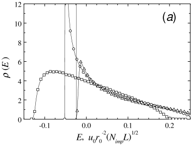
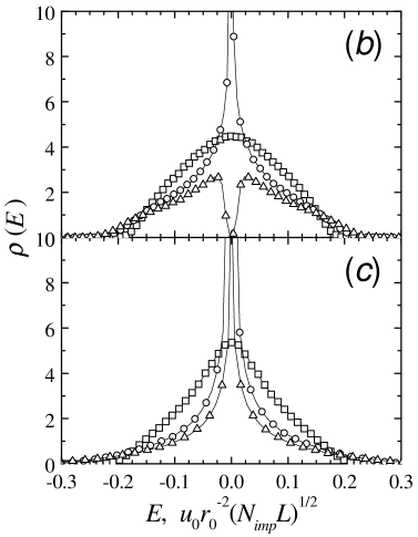
FIG. 3.: The average density of states as a function of energy, measured in units discussed in the text. The data for identical (a), sign-reversal (b) and ND amplitudes (c) are shown. The values of $X$ are $X=4.92\,(\Box)$, $1\,(\circ)$, and $0.62\,(\triangle)$, For convenience of presentation of data with different $L$, the shown DOS is scaled as $\int\rho(E)\,dE=1$ here. The lines are guides to the eye, every second data point is shown. The vertical line on the plot (a) denotes the position of the $\delta-$function for $X=0.62$.

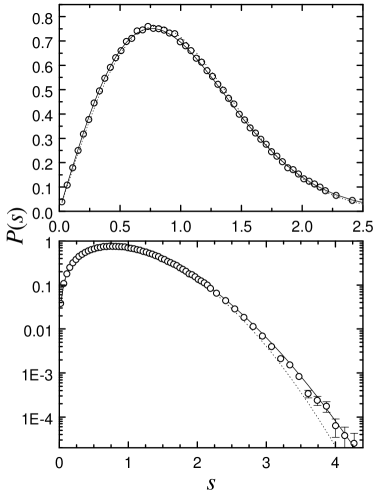
FIG. 4.: Energy spacings distribution for $L=61$, $N_{imp}=300$, identical impurities; $b=1.88$ .

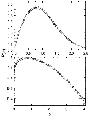
FIG. 5.: Energy spacings distribution for $L=40$, $N_{imp}=50$, identical impurities; $b=1.82$ .

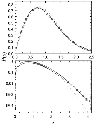
FIG. 6.: Energy spacings distribution for $L=30$, $N_{imp}=50$, “dichotomic” impurities; $b=1.68$ .

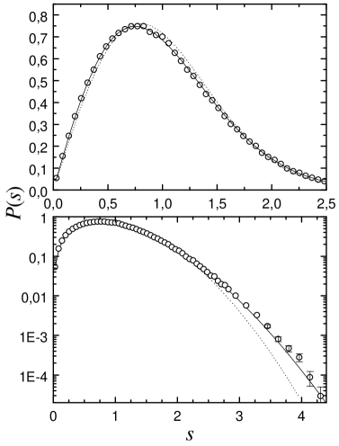
FIG. 7.: Energy spacings distribution for $L=20$, $N_{imp}=200$, ND impurities; $b=1.76$ .

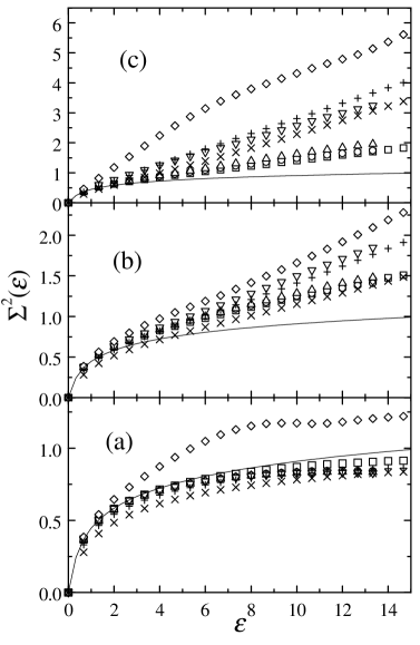
FIG. 8.: Number variance for the amplitudes with (a) fixed value, (b) “dichotomic” and (c) normal distributions. The values of $X$ are : $4.92\,(\Box)$, $4.88\,(\circ)$, $2.93\,(\triangle)$, $1.22\,(\bigtriangledown)$, $1.0\,(\Diamond)$, $0.82\,(+)$, $0.62\,(\times)$. The GOE prediction for the number variance is shown by a solid line.

REFERENCES

- [1] D.Ugarte, Nature 359, 707 (1992) ; M. Zaiser, F. Banhart, Phys.Rev.Letters 79, 3680 (1991).
- [2] N.A. Nicorovici, R.C. McPhedran, G.W. Milton, Phys. Rev. B 49, 8479, (1994) ; K.W.Yu, P.M.Hui, D.Stroud, Phys. Rev. B 47, 14150, (1993).
- [3] W.Ekardt, Phys. Rev. B 34, 526, (1986).
- [4] see, e.g., K.Busch and S.John, Phys.Rev.Lett. 83, 967 (1999) and references therein.
- [5] S.G. Romanov et al., Appl.Phys.Lett. 70, 2091 (1997); Yu.A. Vlasov et al., Phys.Rev. B 55, R13357 (1997).
- [6] A.A.Zakhidov, R.H. Baughman, Z. Iqbal, C. Cui, I. Khayrullin, S.O. Dantas, J. Marti, V.G. Ralchenko, Science 282, 897(1998)
- [7] H Aoki, H Suezawa, Phys.Rev. A 46, R1163 (1992); Ju H Kim, I D Vagner, B Sundaram, Phys.Rev.B 46, 9501 (1992).
- [8] D.N. Aristov, Phys.Rev. B 59, 6368 (1999); JETP Letters 70, 410 (1999).
- [9] D.V. Bulaev, V.A. Geyler, V.A. Margulis, Phys.Rev. B 62, 11517 (2000) and references therein.
- [10] Malits P., Vagner I.D., J. Phys. A : Math. Gen. 32, 1507 (1999).
- [11] C.L. Foden, M.L. Leadbeater, M. Pepper, Phys.Rev.B 52, R8646 (1995).
- [12] D.N. Aristov, Phys. Rev. B 60, 2851 (1999).
- [13] S.R. White, S. Chakravarty, M.P. Gelfand, S.A. Kivelson, Phys.Rev. B 45, 5062 (1992); G.N. Murthy, A. Auerbach, Phys.Rev. B 46, 331(1992); A. Wójs, J.J. Quinn, Physica E 3, 181 (1998) .
- [14] E.M. Baskin, L.I. Magarill, M.V. Entin, Sov. Phys. JETP, 48, 365 (1978).
- [15] T. Ando, J. Phys. Soc. Japan, 36, 1521 (1974).
- [16] V.A. Geyler and V.A. Margulis, Teor. Mat. Fiz., 58, 461 (1984); ibid., 61, 140 (1984).
- [17] D.A. Varshalovich, A.N. Moskalev, V.K. Khersonskii, Quantum Theory of Angular Momentum, (World Scientific, Singapore, 1988).
- [18] V.E.Kravtsov, V.I. Yudson, Phys. Rev. Letters 82, 157 (1999).
- [19] I.M. Lifshits, ZhETF 17, 1017(1947).
- [20] A.G.Aronov, V.E.Kravtsov, I.V.Lerner, Phys. Rev. Letters 74, 1174 (1995) and references therein.
- [21] D. Braun, G. Montambaux, M. Pascaud, Phys. Rev. Letters 81, 1062 (1998).
- [22] M Feingold, Y Avishai, R Berkovits, Phys.Rev. B 52, 8400 (1995);
- [23] R Berkovits, Y Avishai, Phys.Rev. B 53, R16125 (1996);
- [24] B. Huckestein, Rev.Mod.Phys. 67, 357 (1995).
- [25] V.E. Kravtsov, I.V. Lerner, B.L. Altshuler, A.G. Aronov, Phys. Rev. Letters 72, 888 (1994).
- [26] A.G. Aronov, V.E. Kravtsov, I.V. Lerner, JETP Letters 59, 39(1994).
- [27] A.G. Aronov, A.D. Mirlin, Phys. Rev. B 51, 6131 (1995).
- [28] V.E.Kravtsov, I.V.Lerner, Phys. Rev. Letters 74, 2563 (1995).
- [29] J T Chalker, V E Kravtsov, I V Lerner, JETP Letters 64, 386(1996).
- [30] S.N. Evangelou, Phys. Rev. B 49, 16805 (1994).
- [31] A.D. Mirlin, Phys. Rep. 326, 259 (2000).
- [32] see also F. Evers, A.D. Mirlin, Phys. Rev. Lett. 84, 3690 (2000) ; A.D. Mirlin, F. Evers, Phys. Rev. B 62, 7920 (2000).
- [33] B. Huckestein, L. Schweitzer, Phys. Rev. Letters 72, 713 (1994)
- [34] H. Matsuoka, Phys. Rev. B 55, R7327 (1997).
- [35] R.Klesse, M.Metzler, Phys. Rev. Letters 79, 721 (1997).