Towards a realistic microscopic description of highway traffic

Abstract

Simple cellular automata models are able to reproduce the basic properties of highway traffic. The comparison with empirical data for microscopic quantities requires a more detailed description of the elementary dynamics. Based on existing cellular automata models we propose an improved discrete model incorporating anticipation effects, reduced acceleration capabilities and an enhanced interaction horizon for braking. The modified model is able to reproduce the three phases (free-flow, synchronized, and stop-and-go) observed in real traffic. Furthermore we find a good agreement with detailed empirical single-vehicle data in all phases.

Cellular automata (CA) models for traffic flow [1] allow for a multitude of new applications. Since their introduction it is possible to simulate large realistic traffic networks using a microscopic model faster than real time [2, 3]. But also from a theoretical point of view, these kind of models, which belong to the class of one-dimensional driven lattice gases [4], are of particular interest. Driven lattice gases allow us to study generic non-equilibrium phenomena, e.g. boundary-induced phase transitions [5]. Now, almost ten years after the introduction of the first CA models, several theoretical studies and practical applications have improved the understanding of empirical traffic phenomena (for reviews, see e.g. [6, 7, 8, 9, 10, 11]). CA models have proved to be a realistic description of vehicular traffic, in particular in dense networks [2, 3].

Already the first CA model of Nagel and Schreckenberg [1] (hereafter cited as NaSch model) leads to a quite realistic flow-density relation (fundamental diagram). Furthermore, spontaneous jam formation has been observed. Thereby the NaSch model is a minimal model in the sense that any further simplification of the model leads to an unrealistic behaviour. In the last few years extended CA models have been proposed which are able to reproduce even more subtle effects, e.g. meta-stable states of highway traffic [12]. Unfortunately, the comparison of simulation results with empirical data on a microscopic level is not that satisfactory. So far the existing models fail to reproduce the microscopic structure observed in measurements of real traffic [13]. But in highway traffic in particular, a correct representation of the microscopic details is necessary because they largely determine the stability of a traffic state and therefore also the collective behaviour of the system.

From our point of view a realistic traffic model should satisfy the following criteria. First it should reproduce, on a microscopic level, empirical data sets, and second, a very efficient implementation of the model for large-scale computer simulations should be possible. Efficient implementations are facilitated if a discrete model with local interactions is used.

Our approach is based on a driving strategy which comprises four aspects:

• At large distances the cars move (apart from fluctuations) with their desired velocity $v_{max}$.

• At intermediate distances drivers react to velocity changes of the next vehicle downstream, i.e. to “brake lights”.

• At small distances the drivers adjust their velocity such that safe driving is possible.

• The acceleration is delayed for standing vehicles and directly after braking events.

These demands are incorporated by a set of update rules for the $n$th car, characterized by its position $x_{n}(t)$ and velocity $v_{n}(t)$ at time $t$. Cars are numbered in the driving direction, i.e. vehicle $n+1$ precedes vehicle $n$. The gap between consecutive cars (where $l$ is the length of the cars) is $d_{n}=x_{n+1}-x_{n}-l$, and $b_{n}$ is the status of the brake light (on (off) $\rightarrow$ $b_{n}=1(0)$). In our approch the randomization parameter $p$ for the $n$th car can take on three different values $p_{0}$, $p_{d}$ and $p_{b}$, depending on its current velocity $v_{n}(t)$ and the status $b_{n+1}$ of the brake light of the preceding vehicle $n+1$:

$$p=p(v_{n}(t),b_{n+1}(t))=\left\{\begin{array}[]{lll}p_{b}&{\rm if\ }b_{n+1}=1{\rm\ and\ }t_{h}<t_{s}\\ p_{0}&{\rm if\ }v_{n}=0\\ p_{d}&{\rm in\ all\ other\ cases}.\end{array}\right.$$ (1)

where $t_{h}$ and $t_{s}$ are defined later. The update rules then are as follows:

1. Determination of the randomization parameter:
   $p=p(v_{n}(t),b_{n+1})$

2. Acceleration:
   if $((b_{n+1}=0)$ and $(b_{n}=0))$ or $(t_{h}\geq t_{s})$ then:   $v_{n}(t+1)=\min(v_{n}(t)+1,v_{max})$

3. NaSch braking rule:
   $v_{n}(t+1)=\min(d_{n}^{(eff)},v_{n}(t))$
   if $(v_{n}(t+1)<v_{n}(t))$ then:    $b_{n}=1$

4. Randomization, braking:
   if $(rand()<p)$ then:    $v_{n}(t+1)=\max(v_{n}(t+1)-1,0)$
   if $(p=p_{b})$ then:    $b_{n}=1$

5. Car motion:
   $x_{n}(t+1)=x_{n}(t)+v_{n}(t+1)$
   

The velocity of the vehicles is determined by steps $1-3$, while step $0$ determines the dynamical parameter of the model. Finally, the position of the car is shifted in accordance to the calculated velocity in step 4.

In the simulations we introduced a finer discretization than the one usually used in the NaSch model. The length of the cells is given by $1.5$ m which leads to a velocity discretization of $5.4$ km h^-1. Since one time step corresponds to $1$ s, this is slightly above a ‘comfortable’ acceleration of about $\sim 1$ m s^-2 [14]. Each car has a length of $5$ cells.

Although the rules are formulated in analogy to existing models, e.g. the NaSch model, some crucial differences exist. Compared to the NaSch model with velocity-dependent randomization (VDR model) [12], where a velocity dependent randomization step has already been introduced, we even enhanced the action of the braking parameter. Moreover our approach also includes anticipation effects [15, 16], because the effective gap $d_{n}^{(eff)}$ is used instead of the real spatial distance to the leading vehicle.

In order to illustrate the details of our approach we now discuss the update rules stepwise.

1. The braking parameter $p$ is calculated. For a car at rest we apply the value $p=p_{0}$. Therefore $p_{0}$ determines the upstream velocity of the downstream front of a jam. If the brake light of the car in front is switched on and it is found within the interaction horizon we choose $p=p_{b}$. In all other cases we choose $p=p_{d}$.

2. The velocity of the car is enhanced by one unit if the car does not already move with maximum velocity. The car does not accelerate if its own brake light or that of its predecessor is on and the next car ahead is within the interaction horizon.

3. The velocity of the car is adjusted according to the effective gap.

4. The velocity of the car is reduced by one unit with a certain probability $p=p(v_{n}(t),b_{n+1})$. If the car brakes due to the predecessor’s brake light, its own brake light is switched on.

5. The position of the car is updated.

The parameters of the model are the following: the maximal velocity $v_{max}$, the car length $l$, the braking parameters $p_{d}$, $p_{b}$, $p_{0}$, the cut-off time of interactions $h$ and the minimal security gap $gap_{security}$. The action of each parameter will be explained when comparing the simulation results with the empirical data.

The two times $t_{h}=d_{n}/v_{n(t)}$ and $t_{s}=\min(v_{n}(t),h)$, where $h$ determines the range of interaction with the brake light, are introduced to compare the time $t_{h}$ needed to reach the position of the leading vehicle with a velocity-dependent (temporal) interaction horizon $t_{s}$. $t_{s}$ introduces a cutoff which prevents drivers from reacting to the brake light of a predecessor which is very far away. Finally $d_{n}^{(eff)}=d_{n}+\max(v_{anti}-gap_{security},0)$ denotes the effective gap (where $v_{anti}=\min(d_{n+1},v_{n+1})$ is the expected velocity of the leading vehicle in the next time step). The effectiveness of the anticipation is controlled by the parameter $gap_{security}$. Accidents are avoided only if the constraint $gap_{security}\geq 1$ is fulfilled.

The parameter $h$ describes the horizon above which driving is not influenced by the leading vehicle. Several empirical studies reveal that $h$ corresponds to a temporal headway rather than to a spatial one. The estimations for $h$ vary from $6$ s [17], $8$ s [18, 19], $9$ s [20] to $11$ s [21]. Another estimation for $h$ can be obtained from the analysis of the perception sight distance. The perception sight distance is based on the first perception of an object in the visual field at which the driver perceives movement (angular velocity). In [22] velocity-dependent perception sight distances are presented which, for velocities up to $128$ km h^-1, larger than $9$s. We therefore have chosen $h$ to be $6~{}s$ as a lower bound for the time-headway. Besides, our simulations show that correct results can only be obtained for $h\geq 6$. This corresponds to a maximum horizon of $6\times 20$ cells, or a distance of $180$ m, at velocity $v_{max}$.

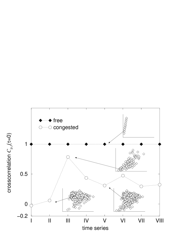
FIG. 1.: Top: Comparison of the local fundamental diagram obtained by a simulation (B) with the corresponding empirical fundamental diagram (A) of [13]. The inset shows the outflow of a megajam. Bottom: Cross-covariance of the flow and the density for different system initialisations. The insets show the corresponding fundamental diagrams. The simulations are performed on a ring with a length of $50000$ cells, each corresponding to $1.5$ m in reality. The parameters of the model are given by $v_{max}=108$ km h^-1 $=20$ cells s^-1, $p=0.1$, $p_{0}=0.5$, $p_{b}=0.94$, $gap_{security}=7$ and $h=6$.

Analogously to the empirical setup the simulation data are evaluated by an virtual induction loop, i.e. we measured the speed and the time-headway of the vehicles at a given link of the lattice. This data set is analysed using the methods suggested in [13]. In particular the density is calculated via the relation $\rho=J/v$ where $J$ and $v$ are the mean flow and the mean velocity of cars passing the detector in a time interval of $1$ min. This dynamical estimate of the density gives correct results only if the velocity of the cars between two measurements is constant, but for accelerating or braking cars, e.g. in stop-and-go traffic, the results do not coincide with the real occupation [13]. In addition to the aggregated data, the single-vehicle data of each car passing the detector are also analysed. Compared to the real part of the highway, analysed in [13], we performed our simulations on a simplified lattice, i.e. we used a single-lane road with periodic boundary conditions. This is justified because the empirical data do not show a significant lane dependence.

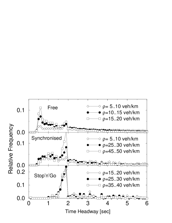
FIG. 2.: Time-headway distribution for different density regimes obtained from computer simulations (top) and from empirical data (bottom). The empirical data are reproduced from [13]. For the simulations we used a periodic lattice and the same set of parameters as in figure 1.

The first goal of a traffic model is to reproduce in detail empirical fundamental diagrams. This is obviously the case for the model proposed here (see figure 1). The empirical fundamental diagram already allows us to determine some of the parameters of the model. The slope of the fundamental diagram in the free-flow regime determines $v_{max}$. Moreover the maximum value of the flow is largely determined by the braking parameter $p$. For the finer discretization used in the simulations we found a reasonable agreement for $v_{max}=20$. The simulated densities are less distributed than in the empirical data set. This observation is simply an artifact of the discretization of the velocities which determines the upper limit of detectable densities.

The next parameter which can be directly related to an empirical observable quantity is the braking parameter $p_{0}$. This parameter determines the outflow of a jam and therefore its upstream velocity. We used the value $p_{0}=0.5$ which leads to an upstream velocity of a compact jam of approximately $12.75$ km h^-1. This velocity is also in accordance with empirical results [23]. Moreover empirical work has revealed that the outflow of a jam is smaller than the maximal possible flow under free-flow conditions [23]. The inset of figure 1 shows that this is well reproduced by the simulations.

A more detailed statistical analysis [13] of the time-series of flux, velocity and density allows for the identification of three different traffic states [23, 24, 25]. Following the arguments of [13] free-flow and congested traffic states can be identified by means of the average velocity. A contiguous time-series of minute averages above $90$ km h^-1 was classified as free flow, otherwise as congested flow. In figure 1 the cross-covariance

$$cc(J,\rho)=\frac{\langle J(t)\rho(t+\tau)\rangle-\langle J(t)\rangle\langle\rho(t+\tau)\rangle}{\sqrt{\langle J^{2}(t)\rangle-\langle J(t)\rangle^{2}}\sqrt{\langle\rho^{2}(t)\rangle-\langle\rho(t)\rangle^{2}}}$$ (2)

of the flow and the local measured density for different traffic states is also shown. In the free-flow regime the flow is strongly coupled to the density indicating that the average velocity is nearly constant. Also for large densities, in the stop-and-go regime, the flow is mainly controlled by density fluctuations. In the mean density region there is a transition between these two regimes. At cross-covariances in the vicinity of zero the fundamental diagram shows a plateau. Traffic states with $cc(J,\rho)\approx 0$ were identified as synchronized flow [13]. In the further comparison of our simulation with the corresponding empirical data we used these traffic states for synchronised flow data and congested states with $cc(J,\rho)>0.7$ for stop-and-go data. The results show that the approach leads to realistic results for the fundamental diagram and that the model is able to reproduce the three different traffic states.

FIG. 3.: Time-headway distribution in the free flow regime of a system with different types of vehicles. The maximal velocity of the slow vehicles is $v_{max}=108$ km h^-1 $=20$ cells s^-1, and of the fast vehicles is $v_{max}=135$ km h^-1 $=25$ cells s^-1. We considered $25\%$ of the vehicles as fast vehicles (note that these are vehicles which disregard the speed limit). The simulations were performed on a lattice of size $L=100000$. Apart from that, the same set of parameters as in figure 1 was used.

Next we compare the empirical data and simulation results on a microscopic level. Measurements of the time-headway distributions are the microscopic equivalents to measurements of the flow. In figure 2 the simulated and empirical time-headway distributions for different density regimes are shown. The time-headways obtained from Monte Carlo simulations are calculated via the relation $\Delta t={\Delta x}/{v}$ with a resolution of $0.1$ s. Due to the discrete nature of the model, large fluctuations occur. In the free-flow state extremely small time-headways have been found, in accordance with the empirical results. Nevertheless, for our standard simulation setup the statistical weight of these small time-headways is significantly underestimated. Therefore we also performed simulations of a system with different types of vehicles. Figure 3 shows that the origin of the peak at small time-headways are fast cars driving in small platoons behind slow vehicles. The location of this peak is mainly influenced by the parameter $gap_{security}$. The results for congested flow, however, are not influenced by different types of vehicles.

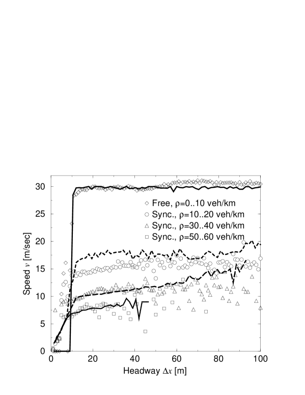
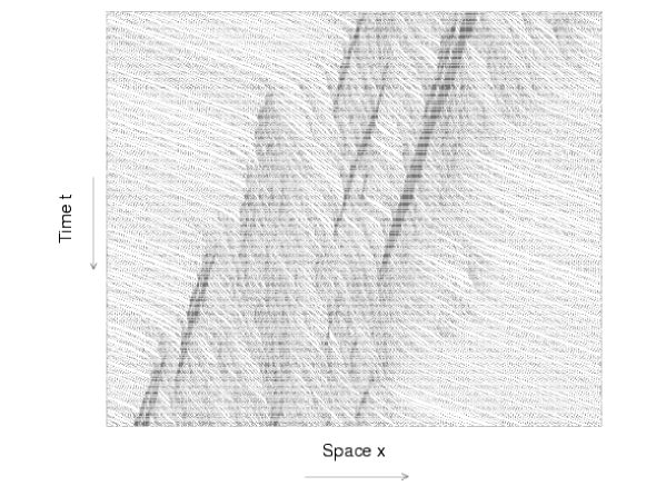
FIG. 4.: Top: The mean speed chosen by the driver as a function of the gap to his predecessor. Comparison of simulations (lines) with empirical data (symbols) [13]. The system size and the parameters comply with figure 1. Bottom: Space-time plot of a periodic system for a global density of $27$ vehicles km^-1. The cars are moving from left to right. Note that the cars have a length of $5$ cells.

The ability to anticipate the predecessor’s behaviour becomes weaker with increasing density so that small time-headways almost vanish in the synchronized and stop-and-go state. Two peaks arise in these states: The peak at a time of $2$ s can be identified with the driver’s efforts for safety: it is recommended to drive with a distance of $2$ s. Nevertheless, with increasing density the NaSch peak at a time of $1$ s (in the NaSch model the minimal time-headway is restricted to $1$ s) becomes dominant. This result is also due to the discretisation of the model which triggers the spatial and temporal distance between the cars. Therefore the continuous part of the empirical distribution shows a peaked structure for the simulations.

For the correct description of the car-car interaction the distance-headway (OV-curve) gives the most important information for the adjustment of the velocities [26]. For densities in the free-flow regime it is obvious that the OV-curve (figure 4) deviates from the linear velocity-headway curve of the NaSch model. Due to anticipation effects, smaller distances occur so that driving with $v_{max}$ is possible even within very small headways. This strong anticipation becomes weaker with increasing density and cars tend to have smaller velocities than the headway allows so that the OV-curve saturates for large distances. The saturation of the velocity, which is characteristic for synchronized traffic, was not observed in earlier approaches. The value of the asymptotic velocities can be adjusted by the last free parameter $p_{b}$.

The simulation results of the approach show that the empirical data are reproduced in great detail. We observed three qualitatively different microscopic traffic states which are in accordance with the empirical results (see the space-time plot in figure 4). The deviations of the simulation results are mainly due to simple discretization artifacts which do not reduce the reliability of the simulation results. We also want to stress the fact that the agreement is on a microscopic level.

This improved realism of our approach leads to a larger complexity of the model compared to other models of this type [27]. Nevertheless, due to the discreteness and the local car-car interactions, very efficient implementations should still be possible. Moreover, the adjustable parameter of the model can be directly related to empirical quantities. The detailed description of the microscopic dynamics will also lead to a better agreement of simulations with respect to empirical data for macroscopic quantities, e.g., jam-size distributions. Therefore we believe that this approach should allow for more realistic micro-simulations of highway networks.

The authors have benefited from discussions with L. Neubert, R. Barlović and T. Huisinga. L. Santen acknowledges support from the Deutsche Forschungsgemeinschaft under Grant No. SA864/1-1. We also thank the Ministry of Economic Affairs, Technology and Transport of North-Rhine Westfalia as well as to the Federal Ministry of Education and Research of Germany for financial support (the latter within the BMBF project “SANDY”).

REFERENCES

- [1] Nagel K and Schreckenberg M 1992 J. Physique 2 2221
- [2] Esser J and Schreckenberg M 1997 Int. J. Mod. Phys. C 8 1025
- [3] Nagel K, Esser J and Rickert M 2000 Annual Review of Computational Physics 7, ed D Stauffer (Singapore: World Scientific) p 151
- [4] Schmittmann B and Zia R K P 1998 Phys. Rep. 301 45
- [5] Krug J 1991 Phys. Rev. Lett. 67 1882
-
[6]
Chowdhury D, Santen L and Schadschneider A 1999
Curr. Sci. 77 411
Chowdhury D, Santen L and Schadschneider Phys. Rep. 329 199 - [7] Helbing D 1997 Verkehrsdynamik: Neue Physikalische Modellierungskonzepte (Berlin: Springer) (in German)
- [8] Wolf D E, Schreckenberg M and Bachem A (ed) 1996 Traffic and Granular Flow (Singapore: World Scientific)
- [9] Schreckenberg M and Wolf D E (ed) 1998 Traffic and Granular Flow ’97 (Berlin: Springer)
- [10] Kerner B S 1999 Phys. World 8 August, p 25
- [11] Kerner B S 1998 Traffic and Granular Flow ’97 ed M Schreckenberg and D E Wolf (Berlin: Springer) p 239
- [12] Barlovic R, Santen L, Schadschneider A and Schreckenberg M 1998 Eur. Phys. J 5 793
- [13] Neubert L, Santen L, Schadschneider A and Schreckenberg M 1999 Phys. Rev. E 60 6480
- [14] Institute of Transportation Engineers 1992 Traffic Engineering Handbook (Washington, DC Institute of Transportation Engineers)
- [15] Knospe W, Santen L, Schadschneider A and Schreckenberg M 1999 Physica A 265 614
- [16] Barrett C L, Wolinsky M and Olesen M W 1996 Traffic and Granular Flow ed D E Wolf, M Schreckenberg and A Bachem (Singapore: World Scientific) p 169
- [17] George H P 1961 Bureau of Highway Traffic, Yale University p 43
- [18] Miller A J 1961 J. R. Stat. Soc. ser B 1 23
- [19] Schlums J 1955 Untersuchungen des Verkehrsablaufes auf Landstraßen (Hannover: Eigenverlag)
- [20] Bureau of Public Roads 1965 Highway Capacity Manual (HRB Spec. Rep. 87) (Washington, DC: U.S. Department of Commerce)
- [21] Edie L C and Foote R S 1958 Proc. HRB 37 334
- [22] Pfefer R C 1976 Transport. Engng J. Am. Soc. Civil Engrs 102 no TE4, 683–97
- [23] Kerner B S and Rehborn H 1996 Phys. Rev. E 53 1297
- [24] Kerner B S 1998 Phys. Rev. Lett. 81 3797
- [25] Kerner B S and Rehborn H 1997 Phys. Rev. Lett. 79 4030
- [26] Bando M and Hasebe K 1995 Phys. Rev. E 51 1035
- [27] Knospe W, Santen L, Schadschneider A and Schreckenberg M in preparation.