Limits of the dynamical approach to non-linear response of mesoscopic systems

Abstract

We have considered the nonlinear response of mesoscopic systems of non-interacting electrons to the time-dependent external field. In this consideration the inelastic processes have been neglected and the electron thermalization occurs due to the electron exchange with the reservoirs. We have demonstrated that the diagrammatic technique based on the method of analytical continuation or on the Keldysh formalism is capable to describe the heating automatically. The corresponding diagrams contain a novel element, the loose diffuson. We have shown the equivalence of such a diagrammatic technique to the solution to the kinetic equation for the electron energy distribution function. We have identified two classes of problems with different behavior under ac pumping. In one class of problems (persistent current fluctuations, Kubo conductance) the observable depends on the electron energy distribution renormalized by heating. In another class of problems (Landauer conductance) the observable is insensitive to heating and depends on the temperature of electron reservoirs. As examples of such problems we have considered in detail the persistent current fluctuations under ac pumping and two types of conductance measurements (Landauer conductance and Kubo conductance) that behave differently under ac pumping.

I Introduction

Recently there has been a considerable interest in non-equilibrium mesoscopics. The effect of adiabatic charge pumping [1] has been experimentally observed [2] and discussed theoretically [3]. Weak localization in a quantum dot under ac pumping has been theoretically studied [4]. The non-equilibrium noise has been suggested [5, 6] as a cause of both the low temperature dephasing saturation [7] and the anomalously large ensemble averaged persistent current [8]. The results of Ref.[6] are based on the earlier works [9] on the ensemble averaged dc current caused by the quantum Aharonov-Bohm rectification of the external ac electric field. Without the Aharonov-Bohm magnetic flux the rectified dc current or voltage (‘photovoltaic effect’) has zero ensemble average but can exist in individual mesoscopic samples because of the specific arrangement of impurities or irregularities in the dot’s shape. This effect was suggested long ago [10] and reconsidered very recently for the case of the quantum dot [11].

Theoretical description of all the effects listed above requires to go beyond the linear response theory and to consider the essentially non-linear response to the ac pump field. This raises a question on the ‘minimal model’ for the adequate description of nonlinear responses in mesoscopic systems. For the linear conductance the minimal model is the system of non-interacting electrons with the impurity scattering and interaction with the external electric field. Such a model does not explicitly contain dissipation. Yet it allows to obtain a correct value of conductivity that is the key quantity for the dissipation function. We will refer to a description based on a model of that sort as the ‘dynamical approach’. In this approach the electron-electron (e-e) and electron-phonon (e-ph) interaction is neglected and the stationary regime under external pumping is reached in an open system via the escape of ‘hot’ electrons into the massive leads playing a role of an electron bath.

The question we address in this paper is this: To what extent this model applies to the nonlinear phenomena in mesoscopic systems and how one can see its limitations through intrinsic inconsistencies and physical paradoxes.

Another important issue we address in this paper is how to describe heating effects by the impurity diagammatic technique without explicitly solving the kinetic equation. It turns out that heating can be described automatically by the new class of diagrams containing the ‘loose diffusons’ with one free end. They are contrasted to the ordinary diffusons and cooperons which are connected in loops by the ‘Hikami boxes’ and describe the effect of electron phase-coherence. Thus we show the way to separate the heating and the dephasing effects on the level of the impurity diagrammatic technique.

The paper is organized as follows. In Sec.II and Sec.III we discuss the general structure of the perturbation theory in the external ac field using the method of analytical continuation and the Keldysh technique and describe simple rules of the impurity diagrammatic technique in the time domain. In Sec.III we derive the diffusion propagators (‘diffusons’ and ‘cooperons’) in the external ac field at different boundary conditions. Sec.IV is central for the paper. There we introduce the ‘loose diffusons’ and demonstrate that evaluating the diagrams with the loose diffusons is equivalent to the solution of the kinetic equation for the electron energy distribution. We also discuss the paradoxes connected with the loose diffusons in closed electronic systems. As an example of the role of the loose diffusons we consider in Sec.V the variance of the persistent current fluctuations under ac pumping. For mesoscopic rings connected to an electron reservoir by a passive lead we compute the temperature dependence of the persistent current fluctuations in equilibrium and under the harmonic ac pumping. In Sec.VI we consider the problem of dc conductance under ac pumping in two different experimental geometries that correspond to measurements of the Landauer and the Kubo conductances. We re-derive the expression for the Landauer conductance in terms of the electron Green’s function in the time domain and show that the loose diffusons cannot be build in this problem. It means that in systems of non-interacting electrons the Landauer conductance is insensitive to the electron energy distribution inside the mesoscopic system and thus is insensitive to heating. In contrast to that the Kubo conductance is sensitive to the non-equilibrium electron distribution in the corresponding system. In Conclusion we summarize the main results of the paper and point out on its obvious extensions.

II Analytical structure of the nonlinear dynamical response

In this section we describe the general analytical structure of the non-linear response of an arbitrary order in the external field using the formalism of the analytical continuation [12] and the Keldysh diagrammatic technique [13, 14]. We will show that causality encoded in the triangular matrix structure of the Green’s functions in the Keldysh technique, allows at most one point where the string of retarded electron Green’s functions is switched to the string of advanced Green’s functions in the expression for the non-linear response of an arbitrary order.

A Causality of a non-linear response and the method of analytical continuation

The formalism of analytical continuation is based on the explicit assumption of causality. One starts with the electron Green’s function ${\cal G}_{\varepsilon,\varepsilon-\omega}$ defined on the Matsubara discrete frequencies $\varepsilon_{n}=\pi T(2n+1)$, $\omega_{n}=2\pi Tn$ ($T$ is the bath temperature) and expanded in series in the ac field ${\bf A}_{\omega}$. Any (local in time) observable is expressed through the sum $T\sum_{\varepsilon}{\cal G}_{\varepsilon,\varepsilon-\omega}$. The non-linear term of the $k$-th order in this sum is $\sum_{\omega^{(i)}}K(i\omega^{(1)},...i\omega^{(k)})\,{\bf A}_{\omega^{(1)}}...{\bf A}_{\omega^{(k)}}$, where $\omega^{(i)}=2\pi T\,n_{i}$ and:

  

$$K(i\omega^{(1)},...,i\omega^{(k)})=T\sum_{\varepsilon}G_{0}(i\varepsilon)G_{0}(i\varepsilon-i\omega^{(1)})G_{0}(i\varepsilon-i\omega^{(1)}-i\omega^{(2)})...\,G_{0}(i\varepsilon-i\omega).$$ (1)

  

In the above equation we omitted the current operators $\hat{{\bf j}}$ or the position operators $\hat{{\bf r}}$ coupled to the vector-potential ${\bf A}_{\omega}$ or to the electric field ${\bf E}_{\omega}=i\omega{\bf A}_{\omega}$ in the electron-field interaction:

$${\cal H}_{\rm e-f} = \left\{\matrix{-{\bf\hat{j}}{\bf A}_{\omega}&{\rm transverse\;\;gauge}\cr-\hat{{\bf r}}\,{\bf E}_{\omega}&{\rm longitudinal\;\;gauge}\cr}\right.$$ (2)

and introduced the exact electron Green’s function in the absence of the time-dependent perturbation:

$$G_{0}(i\varepsilon)=\sum_{m}\frac{\Psi_{m}({\bf r})\Psi_{m}^{*}({\bf r^{\prime}})}{i\varepsilon-\varepsilon_{m}},$$ (3)

where $\Psi_{m}({\bf r})$ is an exact electron wavefunction in the mesoscopic system that corresponds to the stationary state with the energy $\varepsilon_{m}$.

Causality requires the physical (retarded) response function $K(\omega_{1},...\omega_{k})$ which depends on the continuous frequencies $\omega_{i}$, to have no singularities in the upper half-plain of ${\it each}$ complex variable $\omega_{i}$. Thus $K(\omega_{1},...\omega_{k})$ is obtained by the analytical continuation of $K(i\omega^{(1)},...,i\omega^{(k)})$ from the imaginary discrete points $\omega_{i}=i\omega^{(i)}$ into the upper half-plane $\Im\omega_{i}>0$. In order to implement the analytical continuation one represents the sum over $\varepsilon_{n}$ in Eq.(1) as a contour integral over the contour ${\cal C}$ that comprises all the points $i\varepsilon_{n}=i\pi T(2n+1)$ (see Fig.1a):

$$K(i\omega^{(1)},...,i\omega^{(k)})=\int_{{\cal C}}\frac{d\varepsilon}{4\pi i}\,\tanh\left(\frac{\varepsilon}{2T}\right)$$ (4)

$$\times G_{0}(\varepsilon)G_{0}(\varepsilon-i\omega^{(1)})G_{0}(\varepsilon-i\omega^{(1)}-i\omega^{(2)})...$$ (5)

The next step is to deform the contur along the cuts $\Im\varepsilon=0$, $\Im\varepsilon=\omega^{(1)}$, $\Im\varepsilon=\omega^{(1)}+\omega^{(2)}$ and so on (Fig.1b).

In doing that one has to take care of the analytical properties of the electron Green’s functions $G_{0}(\varepsilon)$: the integrand in Eq.(4) should be regular in each strip between the neighbour cuts. This means that for $\Im\varepsilon$ larger than that of the upmost cut all the Green’s functions $G_{0}$ should be chosen retarded $G_{0}^{R}$. In the strip just below this cut one Green’s function with the argument that takes zero value on this cut should be switched to the advanced $G_{0}^{A}$. In the next stripe another retarded Green’s function is switched from the retarded to the advanced one and so on. Thus for $\Im\varepsilon<0$ all the retarded Green’s functions are replaced by the advanced ones.

FIG. 1.: Contours of integration: (a) initial, (b) after deformation along the cuts. The analytical properties [retarded (R) or advanced (A)] of Green’s functions are also shown in each strip.

The next step is to shift the integration from along the cuts to the real axis $-\infty<E<+\infty$. To this end we shift the variable of integration $\varepsilon\rightarrow E+i(\omega^{(1)}...+\omega^{(p)})$ corresponding to the $(p+1)$-th cut $\Im\varepsilon=\omega^{(1)}+...+\omega^{(p)}$. Note that since $i\omega^{(i)}$ is a period of $\tanh(\varepsilon/2T)$ the above shift of variables does not change $\tanh(\varepsilon/2T)\rightarrow\tanh(E/2T)$. As a result we get in the r.h.s. of Eq.(4) a sum of the form:

$$\sum_{p=0}^{k} \left\{G_{0}^{R}(E+i(\omega^{(1)}+...+\omega^{(p)}))...G_{0}^{R}(E+i\omega^{(p)})\right.$$ (6)

$$\times [\,G_{0}^{R}(E)-G_{0}^{A}(E)]\,\tanh\left(\frac{E}{2T}\right)$$ (7)

$$\times \left.G_{0}^{A}(E-i\omega^{(p+1)})...G_{0}^{A}(E-i(\omega^{(p+1)}+...\omega^{(k)}))\right\}.$$ (8)

Now we are in a position to implement the analytical continuation. It reduces simply to the replacement $i\omega^{(i)}\rightarrow\omega_{i}$ because all the Green’s functions have the analytical properties that guarantee the regularity of each term in the sum Eq.(6) in the upper half-plane of each of the complex variables $\omega_{i}$.

One immediately notices the characteristic feature of Eq.(6): it is a sum of products (strings) of Green’s functions such that each string is a product of $p$ functions $G_{0}^{R}$ followed by the product of $k-p+1$ functions $G_{0}^{A}$. There is only one point in each string where the change of the character of analyticity occurs. This property can be traced back to the causal nature of the non-linear response.

B The Keldysh diagrammatic technique

The analytical structure identical to Eq.(6) arises in the Keldysh technique from the triangular matrix structure of electron Green’s functions [15, 14]:

$${\underline{G}}=\left(\begin{array}[]{cc}G^{\rm R}&G^{\rm K}\\ 0&G^{\rm A}\end{array}\right),$$ (11)

where the superscript $K$ stands for the Keldysh component that determines all the observables $O$:

$$O(t)=i{\rm Tr}\left\{{\hat{O}}\,G^{K}(t,t)\right\}.$$ (12)

Treating the applied ac field as a classical field, we assign [15, 14] the matrix vertex $\tau^{0}{\cal H}_{\rm e-f}$ to the electron–field interaction ${\cal H}_{\rm e-f}$, where $\tau^{0}$ is the unit matrix in the $2\times 2$ Keldysh space.

Using the usual expansion of electron Green’s function $\underline{G}$ in powers of electron–field interaction:

$$O(t)=i\sum_{p=0}^{\infty}{\rm Tr}\left\{{\hat{O}}\left[\left\{{\underline{G}}_{0}{\cal H}_{\rm e-f}\right\}^{p}{\underline{G}}_{0}\right]^{\rm K}\right\}_{tt}$$ (13)

$$= i\sum_{p=0}^{\infty}\sum_{l=0}^{p}{\rm Tr}\left[{\hat{O}}\left\{G_{0}^{\rm R}{\cal H}_{\rm e-f}\right\}^{l}G_{0}^{\rm K}\left\{{\cal H}_{\rm e-f}G_{0}^{\rm A}\right\}^{p-l}\right]_{tt},$$ (14)

and the ansatz [15, 14]:

$$G_{0}^{K}(E)=\left[G_{0}^{R}(E)-G_{0}^{A}(E)\right]\,\tanh\left(\frac{E}{2T}\right)$$ (15)

one immediately obtains the same R-A structure as in Eq.(6).

III Non-linear response in the time domain

A Non-locality of perturbation series in the time domain

Let us consider the structure of the expansion Eq. (13), for a given number $p$ of the field vertices, in more detail. This will later help us to establish the structure of an essentially non-linear expessions for different observables in the presence of a time-dependent ac field.

Three different contributions can be distinguished there. In the time–domain representation, the first contribution can be depicted by the electron loop [Fig. 2(a)].

FIG. 2.: Graphic representation of the expansion Eq. (13): (a) retarded, (b) advanced, and (c) retarded–advanced loops. Rays emanating from the electron loops correspond to the electron–field interaction ${\cal H}_{\rm e-f}$, and a triangle stands for the observable operator $\hat{O}$. In the time domain, the factor ${\hat{f}}(\tau)$ is assigned to the $\hat{O}$-vertex in the diagrams (a) and (b). In the diagram (c) this factor is assigned to the retarded–advanced junction shown in bold.

It entirely consists of retarded Green’s functions:

$$+i\int d\tau{\hat{f}}(\tau)\int dt_{1}\ldots dt_{p}{\rm Tr}\left[{\hat{O}}\,G_{0}^{\rm R}(t,t_{1}){\cal H}_{\em e-f}(t_{1})G_{0}^{\rm R}(t_{1},t_{2}){\cal H}_{\rm e-f}(t_{2})\ldots G_{0}^{\rm R}(t_{p-1},t_{p}){\cal H}_{\rm e-f}(t_{p})G_{0}^{\rm R}(t_{p},t-\tau)\right].$$ (16)

The second contribution is associated with the electron loop [Fig. 2(b)] that solely contains advanced Green functions:

$$-i\int d\tau{\hat{f}}(\tau)\int dt_{1}\ldots dt_{p}{\rm Tr}\left[{\hat{O}}\,G_{0}^{\rm A}(t+\tau,t_{1}){\cal H}_{\rm e-f}(t_{1})G_{0}^{\rm A}(t_{1},t_{2}){\cal H}_{\rm e-f}(t_{2})\ldots G_{0}^{\rm A}(t_{p-1},t_{p}){\cal H}_{\rm e-f}(t_{p})G_{0}^{\rm A}(t_{p},t)\right].$$ (17)

The third contribution is associated with the electron loop [Fig. 2(c)] built of $l$ retarded and $(p-l+1)$ advanced Green functions:

$$+ i\int dt_{1}\ldots dt_{l-1}dt_{l+1}\ldots dt_{p}{\rm Tr}\left[{\hat{O}}\,G_{0}^{\rm R}(t,t_{1}){\cal H}_{\rm e-f}(t_{1})\ldots G_{0}^{\rm R}(t_{l-2},t_{l-1}){\cal H}_{\rm e-f}(t_{l-1})\right.$$ (18)

$$\times \,\underbrace{\int d\tau d\tau^{\prime}{\hat{f}}(\tau-\tau^{\prime})\,G_{0}^{\rm R}(t_{l-1},\tau)[{\cal H}_{\rm e-f}(\tau)-{\cal H}_{\rm e-f}(\tau^{\prime})]G_{0}^{\rm A}(\tau^{\prime},t_{l+1})}_{\rm retarded-advanced\,\,junction}\left.{\cal H}_{\rm e-f}(t_{l+1})G_{0}^{\rm A}(t_{l+1},t_{l+2})\ldots{\cal H}_{\rm e-f}(t_{p})G_{0}^{\rm A}(t_{p},t)\right]$$ (19)

  

where

$${\hat{f}}(\tau)=\int\frac{dE}{2\pi}e^{iE\tau}f(E)=\frac{iT}{\sinh(\pi\tau T)}$$ (20)

denotes the Fourier transform of $f(E)=\tanh(E/2T)$.

The characteristic feature of the diagrammatic expansion for an observable in the time domain is that there is one special point (ray) on the loop of Fig.2 which does not correspond to a single point in the time domain. It is the point where the Fourier transform of the energy distribution function is assigned to. Of special importance is the retarded-advanced junction:

$$G_{0}^{R}(t,\tau)\,\hat{f}(\tau-\tau^{\prime})\,[{\cal H}_{\rm e-f}(\tau)-{\cal H}_{\rm e-f}(\tau^{\prime})]\,G_{0}^{A}(\tau^{\prime},t^{\prime}).$$ (21)

It reveals the non-local in the time domain structure of the point [see Fig.2c] where an (arbitrary long) sequence of retarded Green’s functions is switched to an (arbitrary long) sequence of advanced Green’s functions.

B Diffusons and cooperons in the time domain

With the aim to describe the essentially non-linear dependence of observables on the external time-dependent field we introduce the infinite sequence of retarded (advanced) Green’s functions $G_{0}^{R,A}$:

$${\bf G}^{R,A}({\bf r},{\bf r^{\prime}};t,t^{\prime})=\sum_{p=0}^{\infty}\left\{\left[G_{0}^{R,A}\,{\cal H}_{\rm e-f}\right]^{p}\,G_{0}^{R,A}\right\}_{{\bf r},{\bf r^{\prime}};t,t^{\prime}},$$ (22)

where multiplication assumes the convolution over the coordinate and time variables $\{AB\}_{{\bf r},{\bf r^{\prime}};t,t^{\prime}}=\int d{\bf r^{\prime\prime}}dt^{\prime\prime}A_{{\bf r},{\bf r^{\prime\prime}}}(t,t^{\prime\prime})\,B_{{\bf r^{\prime\prime}},{\bf r^{\prime}}}(t^{\prime\prime},t^{\prime})$.

In describing weak localization and mesoscopic phenomena a special role is played by the disorder averages of a pair of electron Green’s functions called ‘diffusons’:

$${\cal D}_{{\bf r}{\bf r^{\prime}}}(t_{+},t^{\prime}_{+};t_{-},t^{\prime}_{-})=\delta(\eta-\eta^{\prime})\,D_{\eta}(t,t^{\prime};{\bf r},{\bf r^{\prime}})$$ (23)

$$= (2\pi\nu\tau_{\rm e})^{-2}\,\langle{\bf G}^{R}({\bf r},{\bf r^{\prime}};t_{+},t^{\prime}_{+}){\bf G}^{A}({\bf r^{\prime}},{\bf r};t_{-}^{\prime},t_{-})\rangle,$$ (24)

and ‘cooperons’:

$${\cal C}_{{\bf r}{\bf r^{\prime}}}(t_{+},t^{\prime}_{+};t_{-},t^{\prime}_{-})=\frac{1}{2}\delta(t-t^{\prime})\,C_{t}(\eta,\eta^{\prime};{\bf r},{\bf r^{\prime}})$$ (25)

$$= (2\pi\nu\tau_{\rm e})^{-2}\langle{\bf G}^{R}({\bf r},{\bf r^{\prime}};t_{+},t^{\prime}_{+}){\bf G}^{A}({\bf r},{\bf r^{\prime}};t_{-},t_{-}^{\prime})\rangle.$$ (26)

In Eqs.(23, 25) $\langle...\rangle$ stands for the disorder average, $\nu$ is the mean electron density of states, $\tau_{\rm e}$ is the electron momentum relaxation time, $t_{\pm}=t\pm\eta/2$, $t^{\prime}_{\pm}=t^{\prime}\pm\eta^{\prime}/2$. The $\delta$-functions in Eqs.(23, 25) result from the assumption on the constant mean density of states over the relevant energy interval much smaller than the electron bandwidth.

In the transverse gauge, the functions $D_{\eta}(t,t^{\prime};{\bf r},{\bf r^{\prime}})$ and $C_{t}(\eta,\eta^{\prime};{\bf r},{\bf r^{\prime}})$ obey the following equations [16] which correspond to the diffusion approximation with $D$ being the diffusion constant:

$$\left\{\frac{\partial}{\partial t}+\gamma+D\left[i\nabla+{\bf A}_{{\bf r}}\left(t+\frac{\eta}{2}\right)-{\bf A}_{{\bf r}}\left(t-\frac{\eta}{2}\right)\right]^{2}\right\}$$ (27)

$$\times D_{\eta}(t,t^{\prime};{\bf r},{\bf r^{\prime}})=\delta(t-t^{\prime})\frac{\delta({\bf r}-{\bf r^{\prime}})}{2\pi\nu\tau_{\rm e}^{2}}.$$ (28)

and

$$\left\{2\frac{\partial}{\partial\eta}+\gamma+D\left[i\nabla+{\bf A}_{{\bf r}}\left(t+\frac{\eta}{2}\right)+{\bf A}_{{\bf r}}\left(t-\frac{\eta}{2}\right)\right]^{2}\right\}$$ (29)

$$\times C_{t}(\eta,\eta^{\prime};{\bf r},{\bf r^{\prime}})=2\delta(\eta-\eta^{\prime})\frac{\delta({\bf r}-{\bf r^{\prime}})}{2\pi\nu\tau_{\rm e}^{2}},$$ (30)

where we assume the electron-field interaction Eq.(2) corresponding to the transverse gauge with the weak space (on the scale of the elastic mean free path $\ell=v_{F}\tau_{\rm e}$) and time (on the scale of $\tau_{\rm e}$) dependence of the external classical field ${\bf A}_{{\bf r}}(t)$ which is also supposed to be weak enough $|{\bf A}_{{\bf r}}(t)|\ell\ll 1$. We also assume the possibility for electrons to escape the mesoscopic system which is described by the (small) escape rate $\gamma$.

C The ring and the quantum dot geometry

Equations (27, 29) should be supplemented by the boundary conditions. Below we consider two principally different geometries shown schematically in Fig.3.

FIG. 3.: The ring (a) and the quantum dot (b) geometry

One of them corresponds to the mesoscopic ring of the circumference $L$ with a small aspect ratio pierced by the time-dependent magnetic field ${\bf H}(t)$ which generates the circular electric field ${\bf E}(t)=-\partial{\bf A}/\partial t$, where ${\bf A}(t)=\frac{1}{2}{\bf H}\times{\bf r}$. In this ring geometry the diffusons and cooperons should obey the periodic boundary conditions.

The ring geometry corresponds to the pumping by the magnetic part of the microwave field when the size of the mesoscopic system $L$ is less than the size of the skin layer. However, for a semiconductor quantum dot with not too large conductivity $\sigma$ the electric part of the microwave field can also penetrate inside the mesoscopic system. For the usual situation $L\ll\lambda$ where $L$ is the size of the system and $\lambda$ is the microwave wavelength the electric field inside the system ${\bf E}(t)=-\partial{\bf A}/\partial t$ is homogeneous in space.

In this situation the boundary conditions read:

$$\left[i\nabla+{\bf Q}^{(d)}(t,\eta)\right]_{{\bf n}}\,D_{\eta}(t,t^{\prime};{\bf r},{\bf r^{\prime}})=0,$$ (31)

$$\left[i\nabla+{\bf Q}^{(c)}(t,\eta)\right]_{{\bf n}}\,C_{t}(\eta,\eta^{\prime};{\bf r},{\bf r^{\prime}})=0,$$ (32)

where ${\bf n}$ is the vector normal to the boundary at a point ${\bf r}$ and we introduce a short-hand notation:

$${\bf Q}^{(d)}(t,\eta)={\bf A}\left(t+\frac{\eta}{2}\right)-{\bf A}\left(t-\frac{\eta}{2}\right),$$ (33)

$${\bf Q}^{(c)}(t,\eta)={\bf A}\left(t+\frac{\eta}{2}\right)+{\bf A}\left(t-\frac{\eta}{2}\right).$$ (34)

D Diffusons and cooperons in the ring geometry

In this case the convenient coordinate $x$ along the ring is proportional to the azimuthal angle $x=L\theta/2\pi$. One can suppress the transverse coordinate, as the dependence on that coordinate at a small aspect ratio is negligible. The tangential component of the field $A_{x}$ is independent on $x$. Given the periodic boundary conditions for diffusons and cooperons, one can switch to the Fourier-transforms $D_{\eta}(t,t^{\prime};q)$ and $C_{t}(\eta,\eta^{\prime};q)$ in Eqs.(27, 29) with the quantized momentum $q_{m}=(2\pi/L)\,m$, where $m=0,\pm 1,\pm 2...$. Then the solution is straightforward:

$$D_{\eta}(t,t^{\prime};q)=\frac{\theta_{t-t^{\prime}}\,e^{-\gamma(t-t^{\prime})}}{2\pi\nu\tau_{\rm e}^{2}}\,e^{-D\int_{t^{\prime}}^{t}d\tau\,\left[q-Q^{(d)}(\tau,\eta)\right]^{2}},$$ (35)

$$C_{t}(\eta,\eta^{\prime};q)=\frac{\theta_{\eta-\eta^{\prime}}\,e^{-\frac{1}{2}\gamma(\eta-\eta^{\prime})}}{2\pi\nu\tau_{\rm e}^{2}}\,e^{-\frac{D}{2}\int_{\eta^{\prime}}^{\eta}d\tau\,\left[q-Q^{(c)}(t,\tau)\right]^{2}},$$ (36)

where $\theta_{t}$ is the step function and $Q^{(d,c)}$ is defined by Eqs.(33, 34).

An important particular case is the zero-mode diffusons $D_{\eta}(t,t^{\prime})=D_{\eta}(t,t^{\prime};q=0)$ and cooperons $C_{t}(\eta,\eta^{\prime})=C_{t}(\eta,\eta^{\prime};q=0)$ which correspond to $q=0$:

$$D_{\eta}(t,t^{\prime})=\frac{\theta_{t-t^{\prime}}e^{-\gamma(t-t^{\prime})}}{2\pi\nu\tau_{\rm e}^{2}}\,e^{-D\int_{t^{\prime}}^{t}d\tau\,\left[{\bf Q}^{(d)}(\tau,\eta)\right]^{2}},$$ (37)

$$C_{t}(\eta,\eta^{\prime})=\frac{\theta_{\eta-\eta^{\prime}}e^{-\frac{1}{2}\gamma(\eta-\eta^{\prime})}}{2\pi\nu\tau_{\rm e}^{2}}\,e^{-\frac{D}{2}\int_{\eta^{\prime}}^{\eta}d\tau\,\left[{\bf Q}^{(c)}(t,\tau)\right]^{2}}$$ (38)

One can see that they decay as a function of $t-t^{\prime}$ or $\eta-\eta^{\prime}$ even at an escape rate $\gamma=0$. This is the manifestation of dephasing by the time-dependent external field. We note that Eq.(23) with $\eta=0$ corresponds to the electron density correlation function. In the absence of electron escape the total number of particles is conserved and therefore $D_{\eta=0}(t,t^{\prime};q=0)$ must be a constant for any $t>t^{\prime}$. This is consistent with the property of $Q^{(d)}(\tau,\eta=0)=0$. However, there is no constraint that would prohibit a decay of $D_{\eta}(t,t^{\prime})$ at a non-zero $\eta$.

E Diffusons and cooperons in the quantum dot geometry.

This case is principally different because of the field-dependent boundary conditions Eqs.(31) and the potential (longitudinal) nature of the electric field inside the dot. This makes the description in the longitudinal gauge more convenient in the quantum dot geometry.

1 Equations for the diffusons and the cooperons in the longitudinal gauge

Performing the gauge transformation:

$$D_{\eta}(t,t^{\prime};{\bf r},{\bf r^{\prime}})=e^{i{\bf Q}^{(d)}(t,\eta){\bf r}}\,\tilde{D}_{\eta}(t,t^{\prime};{\bf r},{\bf r^{\prime}})\,e^{-i{\bf Q}^{(d)}(t^{\prime},\eta){\bf r^{\prime}}},$$ (39)

$$C_{t}(\eta,\eta^{\prime};{\bf r},{\bf r^{\prime}})=e^{i{\bf Q}^{(c)}(t,\eta){\bf r}}\,\tilde{C}_{t}(\eta,\eta^{\prime};{\bf r},{\bf r^{\prime}})\,e^{-i{\bf Q}^{(c)}(t,\eta^{\prime}){\bf r^{\prime}}},$$ (40)

we switch to the longitudinal gauge.

This transformation removes the time-dependent field from the boundary conditions Eq.(31). However, it remains in the equations for $\tilde{D}_{\eta}(t,t^{\prime};{\bf r},{\bf r^{\prime}})$ and $\tilde{C}_{t}(\eta,\eta^{\prime};{\bf r},{\bf r^{\prime}})$ but only as the time-derivatives:

$$\dot{{\bf Q}}(t,\eta) = \frac{\partial}{\partial t}\,{\bf Q}^{(d)}(t,\eta)=2\frac{\partial}{\partial\eta}\,{\bf Q}^{(c)}(t,\eta)$$ (41)

$$= {\bf E}\left(t-\frac{\eta}{2}\right)-{\bf E}\left(t+\frac{\eta}{2}\right),$$ (42)

where ${\bf E}(t)=-\partial{\bf A}(t)/\partial t$.

The operators in the l.h.s. of the corresponding equations take the form:

$$\hat{{\cal L}}_{d}=\left\{\frac{\partial}{\partial t}+\gamma-D\nabla^{2}+i{\bf r}\dot{{\bf Q}}(t,\eta)\right\}$$ (43)

$$\hat{{\cal L}}_{c}=\left\{2\frac{\partial}{\partial\eta}+\gamma-D\nabla^{2}+i{\bf r}\dot{{\bf Q}}(t,\eta)\right\}.$$ (44)

It is convenient to expand $\tilde{D}_{\eta}(t,t^{\prime};{\bf r},{\bf r^{\prime}})$ and $\tilde{C}_{t}(\eta,\eta^{\prime};{\bf r},{\bf r^{\prime}})$ in an infinite sum $\sum_{\nu,\mu}A_{\nu\mu}\,\Phi_{\nu}({\bf r})\Phi_{\mu}(\bf r^{\prime})$ over eigenfunctions $\Phi_{\nu}({\bf r})$ of the diffusion operator $-D\nabla^{2}$ with the Neumann boundary condition [Eq.(31) with ${\bf Q}^{(d,c)}=0$]. Then the equation for the amplitudes $A_{\nu\mu}$ is of the form (for simplicity we consider the case $\gamma=0$ and suppress the redundant indices and variables):

$$\frac{\partial}{\partial t}\,A_{\nu\mu}+E_{\nu}\,A_{\nu\mu}+i\dot{{\bf Q}}(t)\,\sum_{\lambda}{\bf r}_{\nu\lambda}A_{\lambda\mu}=\delta(t-t^{\prime})\delta_{\nu\mu},$$ (45)

where ${\bf r}_{\nu\lambda}$ is the matrix element of the vector ${\bf r}$ in the basis of $\Phi_{\nu}({\bf r})$ and $E_{\nu}$ is the eigenvalue that corresponds to the eigenfunction $\Phi_{\nu}({\bf r})$.

Though this equation looks similar to the (imaginary time) Schrödinger equation for the dynamical Stark effect, identifying $\dot{{\bf Q}}$ as the actual electric field inside the dot would lead to a mistake. Let us consider an important case of the constant in time electric field ${\bf E}$ which corresponds to ${\bf A}(t)=-{\bf E}t$. Then Eqs.(33, 34) give ${\bf Q}^{(d)}(t,\eta)=-{\bf E}\eta$ and ${\bf Q}^{(c)}(t,\eta)=-2{\bf E}t$. One can see from Eq.(41) that in both cases the corresponding time-derivatives $\dot{{\bf Q}}^{(d)}$ and $\dot{{\bf Q}}^{(c)}$ are identically zero!

The conclusion which can be immediately drawn from this observation is that the constant in time longitudinal (potential) electric field cannot lead to a dephasing [cf. Ref.[17]]. This statement is not true for the circular electric field considered above. This field is not constant in the Cartesian coordinates and is not potential ${\bf curl}\;\;{\bf E}\neq 0$.

2 The weak-field adiabatic and anti-adiabatic limits

The general solution to Eq.(45)is unknown even for the space-homogeneous electric field ${\bf E}(t)$ and in the ergodic limit

$$E_{c}(t-t^{\prime})\gg 1\;\;\;\;E_{c}(\eta-\eta^{\prime})\gg 1.$$ (46)

However, one can find a simple approximate solutions in the weak field limit

$$\frac{|\dot{{\bf Q}}|\,L}{E_{c}}\ll 1.$$ (47)

In the ergodic limit Eq.(46) the diffusons $\tilde{D}_{\eta}(t,t^{\prime};{\bf r},{\bf r^{\prime}})$ and cooperons $\tilde{C}_{t}(\eta,\eta^{\prime};{\bf r},{\bf r^{\prime}})$ are nearly space-independent, i.e. the corresponding expansions are dominated by the it zero-mode $\Phi_{0}$ with $E_{0}=0$. By definition the next mode has the eigenvalue equal to the Thouless energy $E_{1}=E_{c}$. For the corresponding amplitude $A_{00}$ we get from Eq.(45):

$$\frac{\partial}{\partial t}A_{00}+i\dot{{\bf Q}}(t)\sum_{\mu\neq 0}{\bf r}_{0\mu}\,A_{\mu 0}=\delta(t-t^{\prime}),$$ (48)

where we choose the system of coordinates in which ${\bf r}_{00}=0$.

In the weak field limit Eq.(47) one can neglect in Eq.(45) $\dot{{\bf Q}}{\bf r}_{\mu\nu}A_{\nu 0}$ compared to $E_{\mu}A_{\mu 0}$ ($\mu,\nu\neq 0$) and obtain the closed system of equations for $A_{00}$ and $A_{\mu 0}$:

$$\frac{\partial}{\partial t}A_{\mu 0}+E_{\mu}A_{\mu 0}+i\dot{{\bf Q}}(t){\bf r}_{\mu 0}\,A_{00}=0.$$ (49)

Solving Eq.(49) and substituting $A_{\mu 0}$ into Eq.(48) we obtain:

$$\frac{\partial}{\partial t}A_{00}+\int_{t^{\prime}}^{t}\dot{{\bf Q}}(t){\bf\Delta}(t-t^{\prime\prime})\dot{{\bf Q}}(t^{\prime\prime})\,A_{00}(t^{\prime\prime},t^{\prime})\,dt^{\prime\prime}=\delta(t-t^{\prime}),$$ (50)

  

where ${\bf\Delta}(t)$ is the matrix in the vector space:

$$[{\bf\Delta}(t)]_{ij}=\sum_{\mu\neq 0}[{\bf r}_{0\mu}]_{i}\,e^{-E_{\mu}t}\,[{\bf r}_{\mu 0}]_{j}.$$ (51)

Eq.(50) can be further simplified in the adiabatic limit where $\dot{{\bf Q}}(t)$ is dominated by the frequencies $\omega\ll E_{c}$. In this case the quantity Eq.(51) can be approximated by the $\delta$-function $[{\bf\Delta}(t)]_{ij}=C_{ij}\delta(t)$, where:

$$C_{ij}=\sum_{\mu\neq 0}[{\bf r}_{0\mu}]_{i}\,[E_{\mu}]^{-1}\,[{\bf r}_{\mu 0}]_{j}.$$ (52)

Then Eq.(50) can be immediately solved and we obtain for the zero-mode amplitudes:

  

$$A^{(d)}_{00}(t,t^{\prime};\eta)=\tilde{D}_{\eta}(t,t^{\prime})=\frac{\theta_{t-t^{\prime}}}{2\pi\nu\tau_{\rm e}^{2}}\,\exp\left[-\int_{t^{\prime}}^{t}\dot{{\bf Q}}^{(d)}_{i}(t^{\prime\prime},\eta)\,C_{ij}\dot{{\bf Q}}^{(d)}_{j}(t^{\prime\prime},\eta)\,dt^{\prime\prime}\right].$$ (53)

$$A^{(c)}_{00}(\eta,\eta^{\prime};t)=\tilde{C}_{t}(\eta,\eta^{\prime})=\frac{\theta_{\eta-\eta^{\prime}}}{2\pi\nu\tau_{\rm e}^{2}}\,\exp\left[-\frac{1}{2}\int_{\eta^{\prime}}^{\eta}\dot{{\bf Q}}^{(c)}_{i}(t,\eta^{\prime\prime})\,C_{ij}\dot{{\bf Q}}^{(c)}_{j}(t,\eta^{\prime\prime})\,d\eta^{\prime\prime}\right].$$ (54)

  

Eqs.(53),(54) are valid in the adiabatic limit $\omega\ll E_{c}$ provided that the conditions Eqs.(46),(47) are fulfilled.

In the opposite anti-adiabatic limit $\omega\gg E_{c}$, the integral term in Eq.(50) is recast as the total time-derivative (which has zero time average and thus strongly oscillates) and the remainder consisting of the strongly oscillating term $-{\bf Q}(t){\bf\Delta}(0)\dot{\bf Q}(t)A_{00}(t,t^{\prime})$ and the term

$$-\int_{t^{\prime}}^{t}dt^{\prime\prime}\;{\bf Q}(t)\,[\partial/\partial t{\bf\Delta}(t-t^{\prime\prime})]\,\dot{{\bf Q}}(t^{\prime\prime})A_{00}(t^{\prime\prime},t^{\prime}).$$

that contains a weakly oscillating part. Integrating this term by parts and using the identity $\dot{{\bf\Delta}}(0)=\partial/\partial t[{\bf\Delta}]_{ij}|_{t=0}=-D\delta_{ij}$ one extracts this weakly oscillating part:

$$-{\bf Q}(t)\dot{{\bf\Delta}}(0)\,{\bf Q}(t)\,A_{00}(t,t^{\prime})=D\,[{\bf Q}(t)]^{2}\,A_{00}(t,t^{\prime}).$$ (55)

Not surprisingly, we conclude that in the anti-adiabatic weak-field limit the system does not feel the boundary and the zero-mode diffusons and cooperons in the quantum dot geometry coincide with those in the ring geometry Eqs.(37).

However, in the adiabatic weak-field limit these two geometries are principally different, since the dephasing factor in Eq.(53),(54) contains a quadratic form in the time-derivative $\dot{{\bf Q}}$ and a structural constant that depends on the system size $L$, while the dephasing factor in Eqs.(37) contains a quadratic form in ${\bf Q}$ and is independent of $L$.

F Time-dependent random matrix theory (TRMT)

The zero-mode approximation Eq.(46) is equivalent to the random-matrix theory (RMT). The fact that there are ${\it two}$ different forms, Eqs.(53),(54) and Eqs.(37), of diffusons and cooperons in the zero-mode approximation suggests two different ways of defining the time-dependent RMT. The idea is to define the Gaussian ensembles of time-dependent random matrices which reproduce the expressions Eq.(53),(54) or Eqs.(37). Then so defined TRMT can be applied to describe not only disodered mesoscopic systems with the diffusion motion of electrons (used in the above derivation) but also ballistic quantum dots with the chaotic electron motion.

Before proceeding with the formal derivation we address a possible confusion based on the common wisdom that only systems in the external field with the characteristic frequency $\omega\ll E_{c}$ can be described by the random matrix theory. This statement is valid for a linear response but it is incorrect in the non-linear case. The point is that in the linear case the frequency of the external field enters all diffusons or cooperons as $[Dq^{2}-i\omega]^{-1}$ where $\omega$ is the difference between the energy variables of retarded and advanced electron Green’s functions. Assuming the summation over momenta $q$ and the fact that the first non-zero mode corresponds to $Dq^{2}=E_{c}$ one concludes that at $\omega\ll E_{c}$ the main contribution to the sum over momenta is given by the zero mode with $q=0$. In the non-linear case the situation is more complicated, since ${\cal H}_{\rm e-f}(t)$ in Eq.(22) is a sum of two parts proportional to $e^{i\omega t}$ and $e^{-i\omega t}$. As a result of the frequency fusion $\omega-\omega=0$ in the field-dependent diffuson(cooperon) self-energy part the difference between the energy variables of retarded and advanced electron Green’s functions constituting a difuson(cooperon) may be zero despite $\omega\gg E_{c}$. This is the reason why the high-frequency external field modifies the zero-mode approximation but does not kill it. The two modifications of the TRMT are:

(i) For the conductors of the ring topology and the quantum dots in the anti–adiabatic limit, $\omega\gg E_{c}$, the time dependent RMT is defined by the matrix Hamiltonian

$$H=H_{0}+i\xi(t)V_{a},$$ (56)

where $\xi(t)$ is a real–time dependent function, $N\times N$ random matrix $H_{0}$ belongs to the Gaussian orthogonal ensemble while $V_{a}$ is the real anti-symmetric random matrix (which corresponds to the sign $-$ in Eq.(57)) of the same size,

$$\langle H_{0}^{nm}H_{0}^{n^{\prime}m^{\prime}}\rangle=\frac{N\delta^{2}}{\pi^{2}}[\delta_{mm^{\prime}}\delta_{nn^{\prime}}+\delta_{mn^{\prime}}\delta_{nm^{\prime}}],$$ (57)

$$\langle V_{a,s}^{nm}V_{a,s}^{n^{\prime}m^{\prime}}\rangle=\frac{\delta C}{\pi}[\delta_{mm^{\prime}}\delta_{nn^{\prime}}\mp\delta_{mn^{\prime}}\delta_{nm^{\prime}}],$$ (58)

$\delta$ being the mean level spacing, and $C$ is a non-universal constant to be identified later on. To make a link between the TRMT, Eqs. (56) and (57), and the zero–dimensional approximation Eqs. (3.15) and (3.31), it is useful to introduce the TRMT diffuson, $D_{\eta}(t,t^{\prime})$, and cooperon, $C_{t}(\eta,\eta^{\prime})$, propagators

  

$$\sum_{n,m}\langle G_{nm}^{R}(t_{+},t_{+}^{\prime})G_{mn}^{A}(t_{-}^{\prime},t_{-})\rangle=\left(2\pi\nu\tau_{\rm e}(N)\right)^{2}\delta(\eta-\eta^{\prime})D_{\eta}(t,t^{\prime}),$$ (59)

$$\sum_{n,m}\langle G_{nm}^{R}(t_{+},t_{+}^{\prime})G_{nm}^{A}(t_{-},t_{-}^{\prime})\rangle=\frac{1}{2}\left(2\pi\nu\tau_{\rm e}(N)\right)^{2}\delta(t-t^{\prime})C_{t}(\eta,\eta^{\prime}),$$ (60)

where $G^{R,A}(t,t^{\prime})$ are retarded or advanced Green’s functions that correspond to the matrix Hamiltonian H, $t_{\pm}=t\pm\eta/2,t_{\pm}^{\prime}=t^{\prime}\pm\eta^{\prime}/2$; $\tau_{\rm e}(N)=\pi/(2N\delta)$, and $\nu=1/\delta$. Using the standard method of Refs. [16] (see also Ref.[4]), we derive the following equations for the TRMT propagators:

$$\left\{\frac{\partial}{\partial t}+C\left[\xi\left(t+\frac{\eta}{2}\right)-\xi\left(t-\frac{\eta}{2}\right)\right]^{2}\right\}D_{\eta}(t,t^{\prime})=\frac{\delta(t-t^{\prime})}{2\pi\nu\tau_{e}^{2}(N)},$$ (61)

$$\left\{\frac{\partial}{\partial\eta}+\frac{C}{2}\left[\xi\left(t+\frac{\eta}{2}\right)+\xi\left(t-\frac{\eta}{2}\right)\right]^{2}\right\}C_{t}(\eta,\eta^{\prime})=\frac{\delta(\eta-\eta^{\prime})}{2\pi\nu\tau_{\rm e}^{2}(N)}.$$ (62)

Comparison with the microscopic Eqs. (3.9) and (3.10) [or (3.31)] suggests identifying the phenomenological constant $C$ introduced in Eq. (57) with the diffusion coefficient $D$; the time–dependent function $\xi(t)$ plays the role of the vector potential $A(t)$. This establishes the equivalence between the TRMT and the zero–dimensional limit of the microscopic theory of Sec. III on the perturbative level.

(ii) For the quantum dots in the adiabatic limit, $\omega\ll E_{c}$, the time dependent RMT is defined by the matrix Hamiltonian [4, 11]

$$H=H_{0}+\xi(t)V_{s},$$ (63)

where $\xi(t)$ is a real–time dependent function, $H_{0}$ and $V_{s}$ are statistically independent, $N\times N$, random matrices belonging to the Gaussian orthogonal ensemble [ see Eq. (57) with the sign $+$].

Again, a link between the TRMT, Eqs. (63) and (57), and the zero–dimensional approximation Eqs. (3.29) and (3.33) of the full microscopic theory, is easily established by deriving the equations for TRMT propagators. One obtains [see also Refs.[4, 11]]:

  

$$\left\{\frac{\partial}{\partial t}+C\left[\xi\left(t+\frac{\eta}{2}\right)-\xi\left(t-\frac{\eta}{2}\right)\right]^{2}\right\}D_{\eta}(t,t^{\prime})=\frac{\delta(t-t^{\prime})}{2\pi\nu\tau_{e}^{2}(N)},$$ (64)

$$\left\{\frac{\partial}{\partial\eta}+\frac{C}{2}\left[\xi\left(t+\frac{\eta}{2}\right)-\xi\left(t-\frac{\eta}{2}\right)\right]^{2}\right\}C_{t}(\eta,\eta^{\prime})=\frac{\delta(\eta-\eta^{\prime})}{2\pi\nu\tau_{\rm e}^{2}(N)}.$$ (65)

  

Comparing with the microscopic Eqs. (3.29) and (3.30), we conclude that the non-universal constant $C$ of Eq. (57) has to be identified with the one given by Eq. (3.28); the function $\xi(t)$ plays the role of ac electric field $E(t)$ in Eq. (3.18). Thus, equivalence between the microscopic approach of Sec. III and the TRMT of the form Eq. (63) is proven perturbatively.

IV The ‘loose’ diffusons

In this section we show that starting from the quadratic in the external field order the diagrams of the impurity technique acquire a new feature: one can draw the diffuson with the free end (‘the loose diffuson’) which carries zero momentum and zero frequency. We will show below that it is exactly the element which describes heating by the external field.

A The loose diffusons and the retarded-advanced junctions

The analytical structure of the retarded-advanced junction Eq.(21) leads after the disorder averaging to an unusual object, the ‘loose’ diffuson. Let us consider this object for the simplest ring geometry.

1 Loose diffusons in the ring geometry

Consider the part of a diagram for an observable or a product of observables that contains the retarded-advanced junction (Fig.4a).

FIG. 4.: The retarded–advanced junction (a), and the Green functions’ disorder averaging [(b) and (c)] resulting in the ‘loose’ diffuson shown by the wavy line (d). It ends up with the triangle; one of the triangle apexes is built upon the retarded–advanced junction, see (b) and (c). The diagram (d) corresponds to the disorder averaging depicted in (b). Dashed lines in (b) and (c) denote the diffuson. Because of the vector nature of the vertex ${\cal H}_{\rm e-f}$ in the transverse gauge Eq.(2) the loose diffuson should ‘embrace’ two vertices ${\cal H}_{\rm e-f}$ in order for the integral over the directions of electron velocity to be non-zero.

One can isolate the retarded-advanced junction from the rest of the diagram by performing the disorder averaging as shown in Fig.4b,c. As the result the ‘loose diffuson’ is formed (Fig.4d) which originates from the main body of the diagram and terminates at a triangle that consists of the retarded-advanced junction and another field vertex adjacent to it. Given the condition $|{\bf A}_{{\bf r}}(t)|\ell\ll 1$ one can neglect the loose diffusons terminating by a polygon with the number of field vertices larger than two.

We stress that the loose diffuson can be built only using the retarded-advanced junction. Indeed, the triangle in Fig.4d whose edges correspond to the average retarded and advanced Green functions $\bar{G}_{E}^{\rm R(A)}({\bf p})=\int d{\bf r}\langle G_{0}^{\rm R(A)}({\bf r},{\bf r}^{\prime};E)\rangle\,e^{-i{\bf p}({\bf r}-{\bf r}^{\prime})}=(E-\xi_{\bf p}\pm i/(2\tau_{\rm e}))^{-1}$, describes the electron motion on the ballistic scale with the electron momentum relaxation time $\tau_{\rm e}$ being the smallest time scale in the problem. One may effectively approximate the average Green’s functions in the time-momentum representation $\bar{G}^{\rm R(A)}({\bf p},t)$ by the $\delta$–functions of the form $\bar{G}^{\rm R(A)}({\bf p},t)\simeq\bar{G}_{E=0}^{\rm R(A)}({\bf p})\delta(t)$. With this approximation and Eq.(21) the triangle in Fig.4d reduces to the quadratic in ${\bf A}(t)$ combination

$$[{\bf A}(t_{1}^{\prime})-{\bf A}(t_{1})]\,{\bf A}(t_{1}^{\prime})\,\hat{f}(t_{1}^{\prime}-t_{1})$$ (66)

multiplied by a constant ($d$ is the dimensionality of momentum space)

$$(v_{F}^{2}/d)\nu\int d\xi({\bf p})\bar{G}_{E=0}^{\rm R}({\bf p})\,[\bar{G}_{E=0}^{\rm A}({\bf p})]^{2}=2\pi i\nu D\tau_{\rm e}.$$ (67)

The triangle that corresponds to Fig.4c is given by:

$$-2\pi i\nu D\tau_{\rm e}\,[{\bf A}(t_{1}^{\prime})-{\bf A}(t_{1})]\,{\bf A}(t_{1})\,\hat{f}(t_{1}^{\prime}-t_{1}).$$ (68)

Without the retarded-advanced junction, all the Green’s functions in the triangle would have the same analyticity ($\rm R$ or $\rm A$), and the integral over $\xi({\bf p})$ vanishes.

Since in the dynamical approach (e-e and e-ph interactions are neglected) there is at most one retarded-advanced junction per electron loop [see Eq.(18)], there could be not more than one loose diffuson for a diagram describing the disorder-average of a single observable $\langle O(t)\rangle$ and not more than $k$ loose diffusons for a diagram describing the disorder-average of a product of $k$ observables $\langle O_{1}(t_{1})...O_{k}(t_{k})\rangle$.

Each of them is given by:

$${\cal D}(t,\eta) = 2\pi i\nu\tau_{\rm e}D\,\int dt_{1}\int d{\bf r}_{1}[{\bf A}(t_{1}+\eta)-{\bf A}(t_{1})]^{2}$$ (69)

$$\times \hat{f}(\eta)\,D_{-\eta}\left(t+\frac{\eta}{2},t_{1}+\frac{\eta}{2};{\bf r}_{1}-{\bf r}\right),$$ (70)

where $\eta=t^{\prime}-t=t_{1}^{\prime}-t_{1}$ and both contributions Eqs.(67),(68) to the triangle have been summed up together. In the ring geometry only the zero mode part of $D_{\eta}(t,t^{\prime};{\bf r}_{1}-{\bf r})$ survives integration over the coordinate ${\bf r}_{1}$ of the free end and using Eq.(37) we finally obtain ${\cal D}(t,\eta)=i\tau_{\rm e}^{-1}\,\hat{f}(\eta)\Lambda_{\eta}(t)$, where:

$$\Lambda_{\eta}(t)=D\int_{-\infty}^{t}d\xi\,[{\bf A}(\xi+\eta)-{\bf A}(\xi)]^{2}\,e^{-\gamma(t-\xi)}\,\exp{\left\{-D\int_{\xi}^{t}d\xi^{\prime}[{\bf A}(\xi^{\prime}+\eta)-{\bf A}(\xi^{\prime})]^{2}\right\}}.$$ (71)

  

2 Loose diffusons in the quantum dot geometry

Eq.(71) holds also in the quantum dot geometry in the anti-adiabatic case $\omega\gg E_{c}$. In the opposite adiabatic case $\omega\ll E_{c}$ the longitudinal gauge is more convenient than the transverse gauge originally accepted in the paper. Eqs.(53),(54) are nothing but the diffusons and cooperons in the longitudinal gauge in the zero-mode approximation. Using Eq.(21) with ${\cal H}_{\rm e-f}$ corresponding to the longitudinal gauge Eq.(2) the loose diffuson can be represented in terms of the matrix elements $A^{(d)}_{0\mu}$ and $r_{\mu 0}$ as follows:

$${\cal D}(t,\eta) = 2\pi i\nu\tau_{\rm e}\hat{f}(\eta)\int dt_{1}\,[\partial{\bf A}(t_{1}+\eta)/\partial t_{1}-\partial{\bf A}(t_{1})/\partial t_{1}]$$ (72)

$$\times \sum_{\mu\neq 0}A^{(d)}_{0\mu}\left(t+\frac{\eta}{2},t_{1}+\frac{\eta}{2};-\eta\right)\,{\bf r}_{\mu 0},$$ (73)

where $A^{(d)}_{0\mu}$ obeys Eq.(49) with $\dot{{\bf Q}}(t)=\dot{{\bf Q}}(t,-\eta)$ and $A^{(d)}_{00}$ given by Eq.(53).

Solving this equation and using the $\delta$-function approximation for ${\bf\Delta}(t)$ we obtain ${\cal D}(t,\eta)=i\tau_{\rm e}^{-1}\,\hat{f}(\eta)\Lambda_{\eta}(t)$ with:

  

$$\Lambda_{\eta}(t)=\int_{-\infty}^{t}d\xi\,C[{\bf E}(\xi+\eta)-{\bf E}(\xi)]^{2}\,e^{-\gamma(t-\xi)}\,\exp{\left\{-\int_{\xi}^{t}d\xi^{\prime}\,C[{\bf E}(\xi^{\prime}+\eta)-{\bf E}(\xi^{\prime})]^{2}\right\}},$$ (74)

  

where $C[{\bf E}(\xi+\eta)-{\bf E}(\xi)]^{2}$ is the short-hand notation for $[{\bf E}(\xi+\eta)-{\bf E}(\xi)]_{i}C_{ij}[{\bf E}(\xi+\eta)-{\bf E}(\xi)]_{j}$ and ${\bf E}=-\partial{\bf A}/\partial t$ is the time-dependent electric field. We also re-installed the finite escape rate $\gamma$.

B Loose diffusons and the singularity of the quadratic response

Eqs.(71),(74) have similar structure: $\Lambda_{\eta}(t)$ contains a quadratic in the external field pre-factor multiplied by the exponential dephasing factor. Because of the quadratic in ${\bf A}$ pre-factor the loose diffuson does not arise in the linear response theory. However, if one considers the quadratic in ${\bf A}$ response, the loose diffusons must be taken into account while the field-dependent dephasing should be neglected. In this approximation we have:

$$\Lambda_{\eta}(t)=\int_{-\infty}^{t}d\xi\,D[{\bf A}(\xi+\eta)-{\bf A}(\xi)]^{2}\,e^{-\gamma(t-\xi)}$$ (75)

and the similar expression in the quantum dot geometry.

Consider the harmonic pumping ${\bf A}={\bf A}_{0}\cos(\omega t)\,\theta(t)$ that is switched on at $t=0$. Then at a time $t\gg\omega^{-1}$ the loose diffuson averaged over the period is given by:

$$\Lambda_{\eta}(t)=2D{\bf A}_{0}^{2}\,\sin^{2}\left(\frac{\omega\eta}{2}\right)\,\frac{1-e^{-\gamma t}}{\gamma}.$$ (76)

One can see that in the limit $\gamma\rightarrow 0$ the loose diffuson is linear in $t$.

We have already mentioned that the disorder average of the product of $k$ observables contains at most $k$ loose diffusons. Were the linear in $t$ growth in Eq.(76) unrestricted, this would mean that the typical value of a mesoscopic observable grows linearly with the running time. For a particular case of the direct current arising in a mesoscopic ring under ac pumping this statement can be found in Ref.[18].

Another similar statement concerns the steady-state regime when the limit $t\rightarrow\infty$ is taken in Eq.(76) prior to the limit $\gamma\rightarrow 0$. One could argue from Eq.(76) that the typical value of a mesoscopic observable in the steady-state is diverging as $\gamma\rightarrow 0$!

However, Eqs.(71),(74) clearly show that both statements are artefacts of the quadratic approximation. In fact because of the field-induced dephasing the quantity $\Lambda_{\eta}(t)$ defined by Eqs.(71),(74) is always smaller than 1. What is really singular in the limit $\gamma\rightarrow 0$ is the quadratic response susceptibility. However, it does not mean a diverging mesoscopic quantity, since at $\gamma\rightarrow 0$ the region of validity of the quadratic in ${\bf A}$ approximation shrinks to zero.

C Loose diffusons and the electron energy distribution

Note that originating from the retarded-advanced junction Eq.(21) the loose diffuson is proportional to the combination $\hat{f}(\eta)\Lambda_{\eta}(t)$, where $\hat{f}(\eta)$ is essentially the Fourier-transform of the Fermi distribution function. From the procedure of building the loose diffuson it is clear that any diagram with the loose diffuson has a parent-diagram without the loose diffuson. For a particular case of the variance of persistent current in a mesoscopic ring the diagrams of Fig.7 (or Fig.8) with one or two loose diffusons stem from the diagram of Fig.6a (or Fig.6b) that contains no loose diffusons. One can check (see Sec.V) that the sum of all diagrams of the given family is equivalent to replacing $\hat{f}(\eta)$ in the parent diagram by:

$$\hat{F}(t+\eta,t)=[1-\Lambda_{\eta}(t)]\,\hat{f}(\eta).$$ (77)

Consider now the simplest case of the steady-state. It corresponds to the ac pumping switched on at $t=-\infty$. Let us define the time average:

$$\Gamma(\eta)=\left\{\matrix{D\overline{[{\bf A}(t+\eta)-{\bf A}(t)]^{2}}&{\rm ring\;or\;dot\;with\;}\omega\gg E_{c}\cr&\cr C\overline{[{\bf E}(t+\eta)-{\bf E}(t)]^{2}}&{\rm dot\;with}\;\omega\ll E_{c}\cr}\right.$$ (78)

Substituting the time average $\Gamma(\eta)$ for $D[{\bf A}(t+\eta)-{\bf A}(t)]^{2}$ or $C[{\bf E}(t+\eta)-{\bf E}(t)]^{2}$ in Eqs.(71),(74) we obtain the function $\hat{F}(t+\eta,t)=\hat{F}(\eta)$ that depends only on the difference of its arguments:

$$\hat{F}(\eta)=\frac{\gamma\,\hat{f}(\eta)}{\gamma+\Gamma(\eta)}.$$ (79)

We conclude that the loose diffusons amount to the renormalization of the energy distribution function in a parent diagram.

This observation is an example of a generic rule that the ‘loose propagators’ in a filed theory can be eliminated by the proper choice of the initial state (‘vacuum’) that in kinetics includes also the energy distribution function. Eq.(79) gives the form of this distribution for an open dynamical system with no intrinsic relaxation and with the electron escape rate $\gamma$. For the particular case of a harmonic pumping in the quantum dot geometry Eq.(79) has been established in Ref.[11].

The renormalized energy distribution function Eq.(79) retains the property $F(E=\pm\infty)=\pm 1$ of the equilibrium distribution $f(E)=\tanh(E/2T)$. This follows from the fact obvious from Eq.(78) that $\Gamma(\eta\rightarrow 0)=0$. However, the form of the energy distribution is different from $\tanh(E/2T)$ and strongly depends on the spectral content of the pumping field. For low bath temperature $T$ it contains at least two energy scales: the bath temperature $T$ and an additional scale $T_{*}$ set by the condition $\Gamma(1/T_{*})=\gamma$. For a harmonic pumping $\Gamma(\eta)=4\gamma{\cal N}\,\sin^{2}(\omega\eta/2)$, where:

$${\cal N}=\left\{\matrix{\frac{D\overline{{\bf E}(t)^{2}}}{\gamma\omega^{2}}&{\rm ring\;or\;dot\;with\;}\omega\gg E_{c}\cr\ &\cr\frac{C\overline{{\bf E}(t)^{2}}}{\gamma}&{\rm dot\;with}\;\omega\ll E_{c}}\right.$$ (80)

For a strong pumping with ${\cal N}\gg 1$ one finds

$$T_{*}=\omega\sqrt{{\cal N}}.$$ (81)

This result [11] corresponds to the diffusion in the energy space with $T_{*}$ being the displacement and ${\cal N}$ being the number of random-walk steps for the time $\gamma^{-1}$ each with emitting or absorbing the energy $\omega$. In this case the inverse Fourier transform $F(E)$ of $\hat{F}(\eta)$ is dominated by the time intervals near zeros of $\Gamma(\eta)$ and we obtain:

$$F(E)=\frac{1}{2\sqrt{{\cal N}}}\sum_{k=-\infty}^{+\infty}\tanh\left(\frac{E-\omega k}{2T}\right)\,e^{-\frac{|k|}{\sqrt{{\cal N}}}}.$$ (82)

At $T\ll\omega\ll T_{*}$ the function $F(E)$ changes from -1 to +1 over the scale $T_{*}$ which plays a role of the effective electron temperature. However it has a fine structure of sharp small steps with the width of the transition regions being equal to the bath temperature $T$ and the width of the plateaus being equal to $\omega$ (see Fig.5).

FIG. 5.: The anti-symmetric part $F(E)=1-2n(E)$ of the electron energy distribution $n(E)$ for an open mesoscopic system of free electrons under harmonic pumping. Solid line corresponds to ${\cal N}=25$, $\omega=1$, $T=0.1$; the dotted line is $\tanh(E/2T_{*})$.

In case of the white-noise pumping $\Gamma(\eta)=2{\cal N}\gamma=const$ for all $\eta\neq 0$ and we formally obtain $T_{*}\rightarrow\infty$. The same result follows from Eqs.(81),(80) in the limit of a closed system $\gamma\rightarrow 0$. On the diagrammatic level this manifests itself in the identity $\Lambda_{\eta}=1$ that holds in the limit $\gamma\rightarrow 0$ for all $\eta\neq 0$ and causes a cancellation of all the diagrams in the given family [19].

In the absence of dissipation or an electron escape the result that the effective electron temperature in the steady state $T_{*}=\infty$ is trivially correct but is certainly unphysical. It clearly sets the limit of the dynamical approach and shows a necessity to take account of an intrinsic dissipation in closed mesoscopic systems.

D Loose diffusons and the kinetic equation

In this subsection we demonstrate that the function $\hat{F}(t_{1},t_{2})$ defined by Eq.(77) is indeed the solution to the kinetic equation. For simplicity we consider the case of the ring geometry and set $\gamma=0$.

To derive the kinetic equation we start with the left and the right Dyson equations for the $2\times 2$ Greens function ${\underline{G}}$:

$$({\underline{G}}_{0}^{-1}-{\underline{\Sigma}})\otimes{\underline{G}}=\delta({\bf x}_{1}-{\bf x}_{1}^{\prime}),$$ (84)

$${\underline{G}}\otimes({\underline{G}}_{0}^{-1}-{\underline{\Sigma}})=\delta({\bf x}_{1}-{\bf x}_{1}^{\prime}).$$ (85)

Here, the standard notations [14] were adopted with ${\bf x}_{k}=({\bf r}_{k},t_{k})$, and

$$G_{0}^{-1}({\bf x})=i\frac{\partial}{\partial t}-\xi_{{\bf p}=-i{\bf\nabla}_{\bf r}-{\bf A}(t)}.$$ (86)

As the external AC field is a classical field, the components $\Sigma^{\rm K(R,A)}$ of the self energy

$${\underline{\Sigma}}({\bf r}t,{\bf r^{\prime}}t^{\prime})=\left(\begin{array}[]{cc}\Sigma^{\rm R}&\Sigma^{\rm K}\\ 0&\Sigma^{\rm A}\end{array}\right)$$ (89)

are

$$\Sigma^{\rm K(R,A)}=({\bf{\hat{j}}A})({\bf x}_{1})G^{\rm K(R,A)}({\bf x}_{1},{\bf x}_{2})({\bf{\hat{j}}A})({\bf x}_{2}).$$ (90)

Subtracting the two Dyson equations Eq. (IV D) from one another, and taking the Keldysh component of the result, one obtains:

  

$$\left[G_{0}^{-1}({\bf x_{1}})-{G_{0}^{-1}}^{*}({\bf x_{2}})\right]G^{\rm K}({\bf x_{1}},{\bf x_{2}})=\left[\Sigma^{\rm K}\otimes G^{\rm A}-G^{\rm R}\otimes\Sigma^{\rm K}+\Sigma^{\rm R}\otimes G^{\rm K}-G^{\rm K}\otimes\Sigma^{\rm A}\right]({\bf x_{1}},{\bf x_{2}}).$$ (91)

  

Before doing the next step we introduce the time-dependent energy distribution function $n(E,t)=(1/2)[1-f(E,t)]$, where $f(E,t)$ is related to the Keldysh component of the matrix Green function:

$${\bf G}^{\rm K}({\bf r}_{1}t_{1},{\bf r}_{2}t_{2}) = \int d\tau\left[F(t_{1},\tau){\bf G}^{\rm R}({\bf r}_{1}\tau,{\bf r}_{2}t_{2})\right.$$ (92)

$$- \left.{\bf G}^{\rm A}({\bf r}_{1}t_{1},{\bf r}_{2}\tau)F(\tau,t_{2})\right],$$ (93)

$$f(E,t) = \int\frac{d\eta}{2\pi}e^{-iE\eta}F\left(t+\frac{\eta}{2},t-\frac{\eta}{2}\right).$$ (94)

Now we substitute Eqs. (90) and (92) into Eq. (91), and perform the disorder averaging. Using the identity:

$$F(t_{1},t_{2})=\frac{i}{2\pi\nu}\sum_{\bf p}\langle G^{\rm K}({\bf p};t_{1},t_{2})\rangle,$$ (95)

we arrive at the equation

$$\left(\frac{\partial}{\partial t_{1}}+\frac{\partial}{\partial t_{2}}\right)F(t_{1},t_{2})=-D\left[{\bf A}(t_{1})-{\bf A}(t_{2})\right]^{2}F(t_{1},t_{2}).$$ (96)

The latter is easy to solve by introducing the function ${\tilde{F}}(t,\eta)=F(t+\eta/2,t-\eta/2)$, with $t=(t_{1}+t_{2})/2$ and $\eta=t_{1}-t_{2}$ being the Wigner variables:

$$\frac{\partial}{\partial t}{\tilde{F}}(t,\eta)=-D\left[{\bf A}\left(t+\frac{\eta}{2}\right)-{\bf A}\left(t-\frac{\eta}{2}\right)\right]^{2}{\tilde{F}}(t,\eta).$$ (97)

In accordance with Eq. (94), the variable $t$ has a clear meaning of the global running time. We supplement Eq.(97) by the initial condition ${\tilde{F}}(t=-\infty,\eta)={\hat{f}}(\eta)$ to end up with:

$$F(t+\eta,t)={\hat{f}}(\eta)\exp\left\{-D\int_{-\infty}^{t}d\xi\left[{\bf A}(\xi+\eta)-{\bf A}(\xi)\right]^{2}\right\}.$$ (98)

Comparison of Eq. (98) with (71) (at $\gamma=0$) shows that the function $F(t_{1},t_{2})$ is identical to the function $\hat{F}(t_{1},t_{2})$ defined by Eq.(77) which follows from the evaluation of diagrams with loose diffusons.

This proves that the loose diffuson $\Lambda_{\eta}(t)$ determines the time-dependent electron energy distribution function $n(E,t)=(1/2)\,[1-f(E,t)]$:

$$f(E,t)=\int\frac{d\eta}{2\pi}\,e^{-iE\eta}\,\hat{f}(\eta)\,[1-\Lambda_{\eta}(t)],$$ (99)

where $\Lambda_{\eta}(t)$ is given by Eqs.(71),(74).

V Fluctuations of persistent current in mesoscopic metallic rings in and out of equilibrium

For illustration purposes we consider in this section how the general formalism described above works in the particular problem of the persistent current [20] in mesoscopic rings pierced by a constant magnetic flux $\phi$ and subject to ac pumping. Since the disorder-averaged persistent current of non-interacting electrons considered in the grand-canonical ensemble is exponentially small [21] we concentrate on the mesoscopic fluctuations of persistent current at temperatures $T\gg 1/\tau_{\phi}$ where $1/\tau_{\phi}$ is the total dephasing rate including that of the ac pumping. This condition allows to neglect dephasing everywhere but in the loose diffusons which describe the evolution of the electron energy distribution under the ac pumping. We will show by straightforward diagrammatic calculations that Eq.(77) indeed holds if all diagrams of the given family are taken into account. This illustrates how the diagrammatic technique takes care of the correct electron energy distribution in the non-eqilibrium problem.

A Equilibrium fluctuations of persistent currents

We start with the equilibrium fluctuations of persistent currents in order to specify the parent diagrams for the problem considered.

Following a standard route, we express the persistent current in terms of exact retarded and advanced electron Green’s functions $G_{0}^{R(A)}$:

$$I_{\rm PC}=i\int\frac{dE}{2\pi}f(E){\rm Tr}\left[{\hat{j}}_{\alpha}(G_{0}^{R}(E)-G_{0}^{A}(E))\right].$$ (100)

Then the variance of the persistent current fluctuations is given by:

$$\langle I_{\rm PC}^{2}\rangle = 2\int\frac{dE}{2\pi}\int\frac{dE^{\prime}}{2\pi}f(E)f(E^{\prime})$$ (101)

$$\times \left\langle{\rm Tr}\left\{{\hat{\bf j}}G_{0}^{R}(E)\right\}{\rm Tr}\left\{{\hat{\bf j}}G_{0}^{A}(E^{\prime})\right\}\right\rangle.$$ (102)

To perform the impurity averaging in Eq. (101), it is convenient to use a representation [22, 23] in which slow diffusion and fast ballistic modes are explicitly separated from each other. The lowest order (single–loop) diagrams contributing to the persistent current fluctuations are shown in Fig. 6. There, wavy lines correspond to Diffuson (${\cal D}_{k}$) or Cooperon (${\cal C}_{k}$) propagators, while triangles and a square (whose edges correspond to the average Green functions) represent the electron motion on the ballistic scale. On the diffusion scale, the latter are reduced to certain constants.

FIG. 6.: Local (a) and nonlocal (b) single–loop diagrams for the equilibrium persistent current fluctuations. Triangular vertices mark the current operators ${\hat{j}}_{\alpha}$. These are the parent diagrams for the persistent current fluctuations under ac pumping.

Applying conventional rules (e.g., see Ref. [24]), we convert the diagrams in Figs. 6(a) and 6(b) to

  

$$\langle{I_{\rm PC}^{2}}\rangle_{\rm l} = 4\pi\nu D\tau_{\rm e}^{2}e^{2}\int d\eta{\hat{f}}^{2}(\eta)\sum_{m}[{\cal C}_{k_{m-2\phi/\phi_{0}}}(\eta)-{\cal D}_{k_{m}}(\eta)],$$ (104)

$$\langle{I_{\rm PC}^{2}}\rangle_{\rm nl} = (4\pi\nu D\tau_{\rm e}^{2})^{2}e^{2}\int d\eta{\hat{f}}^{2}(\eta)\int d\xi\sum_{m}[k_{m}^{2}{\cal D}_{k_{m}}(\xi){\cal D}_{k_{m}}(\eta-\xi)-k_{m-2\phi/\phi_{0}}^{2}{\cal C}_{k_{m-2\phi/\phi_{0}}}(\xi){\cal C}_{k_{m-2\phi/\phi_{0}}}(\eta-\xi)].$$ (105)

  

Here $k_{m}=(2\pi/L)m$ with $m$ running over all integers represents the spectrum of diffusion modes allowed for conductor with the ring topology, $L$ being the circumference. In Eqs. (6), the contributions of single– and double–diffuson (cooperon) diagrams have been singled out in the time domain, in which

$${\cal D}_{k}(t)\equiv{\cal C}_{k}(t)=\frac{\theta(t)}{2\pi\nu\tau_{\rm e}^{2}}\exp(-Dk^{2}t).$$ (106)

In fact, Eq. (106) allows us to effectively compactify the nonlocal diagrams, Fig. 1(b), so that the total fluctuations $\langle I_{\rm PC}^{2}\rangle$ are solely expressed in terms of the contributions of the local diagrams, Fig. 1(a):

$$\langle I_{\rm PC}^{2}\rangle = 8\pi\nu D\tau_{\rm e}^{2}e^{2}\int d\eta{\hat{f}}^{2}(\eta)\left(D\frac{\partial}{\partial D}+\frac{\partial}{\partial D}D\right)$$ (107)

$$\times \sum_{k_{m}}[{\cal C}_{k_{m}-2\phi/\phi_{0}}(\eta)-{\cal D}_{k_{m}}(\eta)].$$ (108)

The fluctuations of persistent currents, Eq. (107) are manifestly periodic in the flux $\phi$, with the period $\phi_{0}/2$. This can explicitly be displayed by performing the re-summation in Eq. (107) using the Poisson formula:

$$\langle I_{\rm PC}^{2}\rangle = \sum_{n=1}^{\infty}\langle I_{n}^{2}\rangle\sin^{2}\left(2\pi n\frac{\phi}{\phi_{0}}\right)$$ (109)

with

$$\langle I_{n}^{2}\rangle = \frac{4C^{2}n^{2}}{\pi^{1/2}}\left(\frac{e}{\tau_{\rm D}}\right)^{2}\,{\tilde{T}}^{2}\int_{0}^{\infty}\frac{dx}{x^{3/2}}\frac{e^{-n^{2}/(4x)}}{\sinh^{2}(\pi{\tilde{T}}x)},$$ (110)

where ${\tilde{T}}=T/E_{c}$ denotes the electron temperature measured in the units of the Thouless energy $E_{c}=1/\tau_{\rm D}$. For generality we also introduce the coefficient $C$ which is equal to 1 for the case of potential disorder (orthogonal ensemble) considered here and $C=1/2$ for the strong spin-orbit interaction (symplectic ensemble).

Eq.(110) is in a complete correspondence with the earlier results obtained in Refs.[25, 26].

B Effect of ac pumping on the persistent current fluctuations

Now let us assume that a time-dependent circular field ${\bf A}(t)$ [see Fig.3a] is applied to the mesoscopic ring and consider the persistent current fluctuations under ac pumping. The dc current in a ring (overline means the time averaging) $I_{dc}=\overline{I^{(1)}(t)+I^{(2)}(t)}$ can be found using Eqs.(13)-(22) [see also Fig.2]:

$$I^{(1)}(t)=i\int d\eta\,\hat{f}(\eta)\,{\rm Tr}\left\{\hat{{\bf j}}{\bf G}^{R}(t,t-\eta)-\hat{{\bf j}}{\bf G}^{A}(t+\eta,t)\right\},$$ (111)

$$I^{(2)}(t) = i\int dt_{1}\int d\eta\,\hat{f}(\eta)\,[{\bf A}_{\alpha}(t_{1}+\eta)-{\bf A}_{\alpha}(t_{1})]$$ (112)

$$\times {\rm Tr}\left\{\hat{{\bf j}}{\bf G}^{R}(t,t_{1}+\eta)\hat{{\bf j}}_{\alpha}{\bf G}^{A}(t_{1},t)\right\},$$ (113)

where ${\bf G}^{R,A}$ are exact electron Green’s functions in the persence of ac pumping Eq.(22).

One can check that for equilibrium electron Green’s functions Eq.(111) reduces to Eq.(100). The contribution Eq.(112) is present only under ac pumping. It describes two principally different effects of ac pumping. One is the rectification of ac field discussed in Refs.[9, 6]. This effect is similar to the photovoltaic effect in a single-connected geometry [10, 11]. Another one is the heating by ac field which we will study starting from the simplest zero order in the pump field parent diagrams of Fig.6. The heating effect in rectification (or photovoltaic effect) can be studied in a similar way [11] starting from the parent diagrams of the second order in the pump field [10, 11, 27].

The daughter-diagrams with loose diffusons which arise after disorder averaging and correspond to the parent-diagram of Fig.6a. are given in Fig.7. We stress that although the parent diagram of Fig.6a arises as the result of the disorder averaging of $\langle I_{1}^{2}\rangle$, the daughter-diagrams always involve $I_{2}$ that contains the retarded-advanced junction and allows to build the loose diffuson. In a similar way we get the non-local daughter-diagrams that correspond to the parent diagram of Fig.6b.

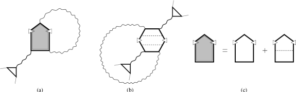
FIG. 7.: Local single–loop daughter-diagrams with one (a) or two (b) loose diffusons contributing to the non-equilibrium fluctuations of persistent current. The diagram (a) arises from the disorder average $\langle I_{1}(t)I_{2}(t^{\prime})\rangle$ and the diagram (b) arises from the disorder average $\langle I_{2}(t)I_{2}(t^{\prime})\rangle$. They are complementary to the parent-diagram of Fig. 6(a). Hikami box of the diagram (a) is detailed in (c).

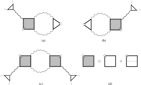
FIG. 8.: Nonlocal single–loop daughter-diagrams: the diagrams (a) and (b) arise from the disorder average of $\langle I_{1}(t)I_{2}(t^{\prime})\rangle$ while the diagram (c) arises from the disorder average $\langle I_{2}(t)I_{2}(t^{\prime})\rangle$. These are complementary to the parent-diagram of Fig. 6(b). The corresponding Hikami box (d) is also shown.

Calculating the diagrams of Fig.7 and Fig.8 and assuming $T\gg\gamma,1/\tau_{\phi}$ we neglect both dephasing and electron escape in the loop diffusons/cooperons and adopt Eq.(106) to describe them. Then summing up all the diagrams of Fig.6-8 we arrive at the expression for the disorder average $\langle I_{PC}(t)I_{PC}(t^{\prime})\rangle$ which is exactly the same as Eq.(107) with $\hat{f}^{2}(\eta)$ replaced by $\hat{f}^{2}(\eta)\,(1-\Lambda_{\eta}(t))(1-\Lambda_{\eta}(t^{\prime}))$. This leads to the ansatz Eq.(77).

In particular, for a harmonic pumping with the frequency $\omega=\tilde{\omega}E_{c}$ we obtain from Eq.(79):

$$\langle I_{n}^{2}\rangle = \frac{4C^{2}n^{2}}{\pi^{1/2}}\left(\frac{e}{\tau_{\rm D}}\right)^{2}\,\int_{0}^{\infty}\frac{dx}{x^{3/2}}e^{-n^{2}/(4x)}\,F^{2}(x),$$ (114)

where

$$F(x)=\frac{\tilde{T}}{\sinh(\pi\tilde{T}x)}\,\frac{1}{\left[1+4{\cal N}\,\sin^{2}\left(\frac{\tilde{\omega}x}{2}\right)\right]}.$$ (115)

Here we assume that the ring is connected to the electron reservoir by a passive lead [see Fig.10b] which results in a finite electron escape rate $\gamma$ and allows to reach a steady-state regime. The escape rate enters the constant ${\cal N}$ in Eq.(80) that is equal to the number of absorption/emission events for the escape time and thus describes the pumping strength.

At $T_{*}=\omega\sqrt{{\cal N}}\gg E_{c}$ the variance of persistent current fluctuations is stongly suppressed but still significantly depends on the bath temperature $T$ even if $T\ll T_{*}$ [see Fig.9].

FIG. 9.: Temperature dependence of the variance of the first harmonic of persistent current in units of $(e/\tau_{D})^{2}$: the equilibrium temperature dependence (upper curve) and two close curves (blown up by a factor of 5) for the non-equilibrium case with $T_{*}=20E_{c}$ corresponding to $\tilde{\omega}=10$, ${\cal N}=4$ and $\tilde{\omega}=2$, ${\cal N}=100$. The temperature dependence is significant in the non-equilibrium case even for $T\ll T_{*}$.

For instance at $\omega\ll E_{c}$ and $T_{*}=\omega\sqrt{{\cal N}}\gg E_{c}$ we obtain

$$\langle I_{n}^{2}\rangle\propto\left(\frac{E_{c}}{T_{*}}\right)^{4}\,\int_{0}^{\infty}\frac{dx}{x^{11/2}}e^{-n^{2}/(4x)}\,\frac{\tilde{T}^{2}}{\sinh^{2}(\pi\tilde{T}x)}$$ (116)

Eq.(116) shows the dependence on the bath temperature $T=\tilde{T}E_{c}$ which is of the same type as in the absence of pumping Eq.(110), only the magnitude of fluctuations decreases by the factor of $(E_{c}/T_{*})^{2}\ll 1$. So the overall width $T_{*}$ and the small steps in the electron energy distribution of Fig.5 manifest themselves in the variance of persistent current fluctuations.

VI dc conductance under ac pumping

In this section we consider the dc conductance in a mesoscopic system under ac pumping. This problem has been recently addressed in the work by Pedersen and Büttiker [28]. Here we neglect the electron interaction and focus on the effect of heating by the ac field. It is well known that the mesoscopic conductance fluctuations are temperature dependent and decrease when the size of the system $L\gg L_{T}$ where $L_{T}=\sqrt{D/T}$. The question we address here is whether or not the effective temperature $T_{*}$ is what should stand for the bath temperature $T$ in the expression for $L_{T}$ under ac pumping. The answer is not obvious in the geometry of an open quantum dot connected by the leads to electron reservoirs [ see Fig.10a,b]. The point is that there are several different electron energy distributions in such a problem. The electron energy distribution in each reservoir is supposed to be the equilibrium Fermi distribution with a certain chemical potential and temperature. In addition, there is the non-equilibrium electron energy distribution inside the dot under ac pumping.

We define the Landauer conductance as the linear dc current response to the difference of the chemical potentials between two different reservoirs with the same temperature [Fig.10a].

Another experimental situation corresponds to measurements of the linear dc current response to the perturbation of the system’s Hamiltonian caused by the constant electric field inside the mesoscopic system. The corresponding response function will be referred to as the Kubo conductance. It can be realized as a current response in a ring that is pierced by a magnetic flux [30] [see Fig.10b].

FIG. 10.: Experimental geometries for the Landauer (a) and Kubo (b) conductances. In the case of Landauer conductance the dc current $I_{0}$ is the response to the chemical potential difference $\mu_{1}-\mu_{2}$ between two reservoirs which enter through the Fermi-distributions of the incoming electrons. In the case of Kubo conductance the dc current $I_{0}$ is the response to the perturbation $\hat{j}E_{0}t$ of the system’s Hamiltonian. The passive lead connects the mesoscopic ring to the electron reservoir with the equilibrium distribution of electrons.

The flux is supposed to contain two parts: one is growing linearly with time and causes the dc electric field. Another one produces the high-frequency pumping.

We will show that these two cases are drastically different (the same conclusion has been reached by Vavilov and Aleiner [29]). The Landauer conductance of non-interacting electrons is insensitive to heating and depends only on the bath temperature $T$. At the same time the non-equilibrium electron energy distribution in the mesoscopic ring does matter for the Kubo conductance. In particular the mesoscopic fluctuations of the Kubo conductance should feel the effective temperature $T_{*}$ rather than the temperature of the electron reservoir $T$ which the mesoscopic ring is connected to by the passive lead.

A Landauer conductance in terms of electron Green’s functions in the time domain

In order to prove the statement on the absence of sensitivity of the Landauer conductance to heating produced by ac pumping in the dot and to see the key difference between the Landauer and the Kubo conductances we re-derive the Landauer conductance to allow for an arbitrary ac pumping. To derive the expression for the Landauer conductance in terms of the electron Green’s functions we proceed along the route used in Ref.[11].

1 Formulation of the Landauer conductance

For simplicity we consider a zero-dimensional dot described by the $N\times N$ random time-dependent matrix $H_{ij}(t)$ connected to two perfect semi-infinite ($x<0$) leads each containing $M$ channels labeled by $\alpha$. There is neither disorder nor electron interaction with each other or with an external ac field inside the leads. Therefore the matrix Green’s function $\underline{G}_{++,\alpha\beta}(t-t^{\prime},x-x^{\prime})$ of the Keldysh technique Eq.(11) for incoming electrons in the leads depends only on the difference of time and coordinates [31]. Moreover, the incoming electrons are supposed to be in equilibrium at the bath temperature $T$ and the chemical potential $\mu+\delta\mu$, where $\delta\mu=\pm U/2$ differs in sign for the leads 1 and 2. Then the Keldysh component $G_{++,\alpha\beta}^{K}(E,x-x^{\prime})$ of the incoming electron Green’s function $\underline{G}_{++,\alpha\beta}(E,x-x^{\prime})$ in the energy-coordinate representation takes the form [cf. Eq.(15)]:

$$G^{K}_{++,\alpha\beta}(E,x-x^{\prime})=\tanh\left(\frac{E-\delta\mu_{\alpha}}{2T}\right)$$ (117)

$$\times [G_{++,\alpha\beta}^{R}(E,x-x^{\prime})-G_{++,\alpha\beta}^{A}(E,x-x^{\prime})].$$ (118)

The retarded and advanced components for incoming electrons $G^{R(A)}_{++,\alpha\beta}(t-t^{\prime},x-x^{\prime})$ in the leads are given by:

$$G^{R}_{++,\alpha\beta} = i\theta(t-t^{\prime})\,\delta_{\alpha\beta}\,\delta(v_{F}(t-t^{\prime})-(x-x^{\prime}))$$ (119)

$$G^{A}_{++,\alpha\beta} = -i\theta(t^{\prime}-t)\,\delta_{\alpha\beta}\,\delta(v_{F}(t-t^{\prime})-(x-x^{\prime})).$$ (120)

Here we linearized the Schrödinger equation near the Fermi momentum and introduced right (incoming) and left (outgoing) movers $\Psi_{\pm}^{(\alpha)}(x,t)=A_{\pm}\,e^{\pm ikx-iv_{F}kt}\,e^{\pm ip_{F}x}$. Then the wave function in the leads $(x<0)$ is:

$$\Psi^{(\alpha)}(x,t)=\Psi_{+}^{(\alpha)}(x,t)+\Psi_{-}^{(\alpha)}(x,t).$$ (121)

The Schrödinger equation for electron states inside the dot $\psi_{n}(t)$ coupled to electron states in the leads $\Psi_{\pm}^{(\alpha)}(x,t)$ is taken in the form:

$$\sum_{m}[i\delta_{nm}\partial_{t}-H_{nm}(t)]\,\psi_{m}(t)=\sum_{\alpha}W^{\dagger}_{n\alpha}\,\Psi^{(\alpha)}(0,t),$$ (122)

where $W_{\alpha n}$ is the $2M\times N$ coupling matrix.

Neglecting electron-electron interaction we introduce the linear boundary conditions at $x=0$:

$$-iv_{F}\,[\,\Psi_{+}^{(\alpha)}(0,t)-\Psi_{-}^{(\alpha)}(0,t)]=\sum_{m}W_{\alpha m}\,\psi_{m}(t),$$ (123)

For massive leads with the semiclassical electron motion, electrons adiabatically turn back at $W_{\alpha m}\rightarrow 0$ acquiring only a certain phase which may be included into the definition of $\Psi_{\pm}^{(\alpha)}$.

Equations Eqs.(122),(123) generate the corresponding equations for the matrix Green’s functions:

$$\sum_{m}[i\delta_{nm}\partial_{t}-H_{nm}(t)]\,\underline{G}_{\pm,m\beta}(t,t^{\prime};x^{\prime})$$ (124)

$$= \sum_{\alpha}W^{\dagger}_{n\alpha}\,[\underline{G}_{+\pm,\alpha\beta}(t,t^{\prime};-x^{\prime})+\underline{G}_{-\pm,\alpha\beta}(t,t^{\prime};-x^{\prime})],$$ (125)

$$\sum_{m}W_{\alpha m}\,\underline{G}_{\pm,m\beta}(t,t^{\prime};x^{\prime})=-iv_{F}$$ (126)

$$\times [\,\underline{G}_{+\pm,\alpha\beta}(t,t^{\prime};-x^{\prime})-\underline{G}_{-\pm,\alpha\beta}(t,t^{\prime};-x^{\prime})],$$ (127)

where the label $+(-)$ corresponds to the incoming (outgoing) electrons in the leads and $\underline{G}_{\pm,m\beta}$ is the ‘cross’ Green’s function of an incoming (outgoing) electron in a channel $\beta$ in the leads and an electron at a site $m$ in the dot.

According to Eq.(12) the current $I_{1,2}(t)$ in the leads 1 or 2 is given by the Keldysh components $G^{K}_{++,\alpha\alpha}(t,t;0)$ and $G^{K}_{--,\alpha\alpha}(t,t;0)$ of the incoming and outgoing electrons:

$$I_{1,2}=iv_{F}\sum_{\alpha\in 1,2}[G^{K}_{++,\alpha\alpha}(t,t;0)-G^{K}_{--,\alpha\alpha}(t,t;0)].$$ (128)

2 Analytical structure of the scattering matrix

It is possible [11] to express the Keldysh component $G^{K}_{--,\alpha\beta}(t,t^{\prime};0)$ of the outgoing electrons in terms of the known Keldysh component $G^{K}_{++,\alpha\beta}(t,t^{\prime};0)$ for the incoming electrons using the time-dependent scattering matrix $S_{\alpha\beta}(t,t^{\prime})$:

$$G^{K}_{--,\alpha\beta}(t,t^{\prime};0)=$$ (129)

$$= \int dt_{1}\int dt_{2}\,S_{\alpha\gamma}(t,t_{1})\,G^{K}_{++,\gamma\delta}(t_{1}-t_{2};0)\,S^{\dagger}_{\delta\beta}(t_{2},t^{\prime}).$$ (130)

It is crucial for us that the scattering matrix $S_{\alpha\beta}(t,t^{\prime})$ involves only the retarded component ${\bf G}^{R}_{mn}(t,t^{\prime})$ of the electron Green’s function inside the dot and the Keldysh component ${\bf G}^{K}_{nm}(t,t^{\prime})$ drops out of the scattering matrix [11]:

$$S_{\alpha\beta}(t,t^{\prime})=\delta_{\alpha\beta}\,\delta(t-t^{\prime})-2iv_{F}^{-1}\,W_{\alpha n}\,{\bf G}^{R}_{nm}(t,t^{\prime})\,W^{\dagger}_{m\beta}.$$ (131)

We remind that only the Keldysh component ${\bf G}^{K}_{nm}(t,t^{\prime})$ contains an information on the electron energy distribution inside the dot. It describes the real transitions between energy levels in the dot which are constrained by the energy conservation law and the Pauli principle. In contrast to that the retarded component ${\bf G}^{R}_{mn}(t,t^{\prime})$ describes virtual transitions where no energy conservation applies and thus the energy distribution function is irrelevant.

Formally the fact that the scattering matrix is independent of ${\bf G}^{K}_{mn}(t,t^{\prime})$ follows from Eqs.(124),(126). Let us express $\underline{G}_{-+,\alpha\beta}$ through $\underline{G}_{++,\alpha\beta}$ and $\underline{G}_{+,m\beta}$ using Eq.(126) and substitute it into Eq.(124). As the result of the transformation $2\underline{G}_{++,\alpha\beta}$ appears in the r.h.s. of Eq.(124) and the matrix Hamiltonian for electrons in the dot acquires an imaginary part $H_{nm}\rightarrow H^{R}_{nm}$, where:

$$H^{R,A}_{nm}=H_{nm}\mp iv_{F}^{-1}\,(W^{\dagger}W)_{nm}.$$ (132)

According to the rules of the Keldysh technique the generic solution $G^{K}_{+,m\beta}$ to the transformed Eq.(124) involves both the combination ${\bf G}^{R}_{mn}W^{\dagger}_{n\alpha}G^{K}_{++,\alpha\beta}$ and the combination ${\bf G}^{K}_{mn}W^{\dagger}_{n\alpha}G^{A}_{++,\alpha\beta}$, where $\underline{\bf G}$ is the marix Green’s function for electrons in the dot, for instance:

$${\bf G}^{R}_{nm}(t,t^{\prime})=\left[i\partial_{t}-H^{R}(t)\right]_{nm}^{-1}.$$ (133)

However, in this particular scattering problem we have:

$$G^{A}_{++,\alpha\beta}(t,t^{\prime};x-x^{\prime}>0)=0.$$ (134)

Eq.(134) follows immediately from the $\delta$-function and the $\theta$- function structure of Eq.(120). Therefore we obtain from Eqs.(124),(126):

$$G^{K}_{-+,\alpha\beta}(t,t^{\prime};0)=\int dt_{1}S_{\alpha\gamma}(t,t_{1})G^{K}_{++,\gamma\beta}(t_{1},t^{\prime};0).$$ (135)

with $S_{\alpha\gamma}(t,t_{1})$ given by Eq.(131) which contains only the retarded component ${\bf G}^{R}_{nm}$ of the electron Green’s function in the dot.

In a similar way one can express $G^{K}_{--,\alpha\beta}(t,t^{\prime};0)$ through $G^{K}_{-+,\alpha\beta}(t,t^{\prime};0)$ using the Hermitean conjugated equations Eq.(124),(126) to finally arrive at Eq.(129).

3 Expression for the Landauer conductance

Now we substitute Eq.(129) in Eq.(128) with $S_{\alpha\beta}(t,t^{\prime})$ given by Eq.(131) to get for the linear dc response current $I_{0}=\overline{I_{\rm lin}(t)}$:

$$I_{\rm lin}(t) = -v_{F}^{-2}\,U\int dt_{1}\int dt_{2}\,[-i(t_{1}-t_{2})\,\hat{f}(t_{1}-t_{2})]$$ (136)

$$\times {\rm Tr}\left\{(1+\Lambda)W{\bf G}^{R}(t,t_{1})W^{\dagger}\Lambda W{\bf G}^{A}(t_{2},t)W^{\dagger}\right\}-$$ (137)

$$+ i(v_{F}^{-1}/2)\,U\int dt_{1}\,[-i(t_{1}-t)\,\hat{f}(t_{1}-t)]$$ (138)

$$\times {\rm Tr}\left\{(1+\Lambda)W[{\bf G}^{R}(t,t_{1})-{\bf G}^{A}(t_{1},t)]W^{\dagger}\right\},$$ (139)

where we have introduced the diagonal matrix $\Lambda$:

$$\Lambda_{\alpha\alpha}=\left\{\matrix{+1,&\alpha\in{\rm lead\;\;1}\cr-1,&\alpha\in{\rm lead\;\;2}\cr 0,&{\rm otherwise}}\right.$$ (140)

Equation Eq.(136) can be simplified using the identity:

$${\bf G}^{R}(t,t^{\prime})-{\bf G}^{A}(t,t^{\prime})=-{\bf G}^{A}\left\{[{\bf G}^{-1}]^{R}-[{\bf G}^{-1}]^{A}\right\}{\bf G}^{R}$$ (141)

$$= -2iv_{F}^{-1}\,\int dt_{1}\,{\bf G}^{A}(t,t_{1})\,W^{\dagger}W\,{\bf G}^{R}(t_{1},t^{\prime})$$ (142)

which is obtained with the help of Eq.(132).

In order to obtain the dc $I_{0}$ one has to average Eq.(136) over $t$ within the observation time ${\cal T}\rightarrow\infty$. This means an additional integration over $t$. Then using the fact that $t\hat{f}(t)$ is an even function one can replace ${\bf G}^{A}(t_{1},t)$ by ${\bf G}^{A}(t,t_{1})$ in the second term of Eq.(136). After that Eq.(141) can be applied to yield:

$$g_{\rm Land}=v_{F}^{-2}\,\int_{-{\cal T}/2}^{+{\cal T}/2}\frac{dt}{{\cal T}}\int dt_{1}\int d\eta\,[-i\eta\,\hat{f}(\eta)]$$ (143)

$$\times {\rm Tr}\left\{-W^{\dagger}(1+\Lambda)\,W{\bf G}^{R}(t,t_{1})W^{\dagger}\Lambda W{\bf G}^{A}(t_{1}+\eta,t)\right.$$ (144)

$$+ \left.W^{\dagger}W{\bf G}^{R}(t,t_{1})W^{\dagger}(1+\Lambda)W{\bf G}^{A}(t_{1}+\eta,t)\right\}.$$ (145)

Finally we assume that the $2M\times N$ coupling matrix $W_{\alpha n}$ has only 2M nonzero matrix elements, those with $\alpha=n$; all these elements are taken equal to W. Then Eq.(143) takes the form:

  

$$g_{\rm Land}=\frac{1}{2}\gamma^{2}\int dt_{1}\int d\eta\,[-i\eta\,\hat{f}(\eta)]\,M^{-2}\,{\rm Tr}\left\{\overline{{\bf G}_{12}^{R}(t,t_{1}){\bf G}_{21}^{A}(t_{1}+\eta,t)}+\overline{{\bf G}_{21}^{R}(t,t_{1}){\bf G}_{12}^{A}(t_{1}+\eta,t)}\right\},$$ (146)

where $\hat{f}(\eta)$ is the Fourier transform of $\tanh(E/2T)$; the overline denotes the average over time $t$; $\gamma=2v_{F}^{-1}|W|^{2}M$ is the electron escape rate, $M$ is the number of channels in each lead and the subscripts 1 or 2 indicate that only sites connected to the first or the second lead should be taken into account in the summation over matrix indices.

Using Eq.(141) one can [4] recast Eq.(146) as a sum of two parts $g_{\rm Land}=g_{1}+g_{2}$ where

  

$$g_{1}=\frac{i}{4}\gamma\int d\eta\,[-i\eta\,\hat{f}(\eta)]\,M^{-1}\,{\rm tr}\left\{\overline{{\bf G}^{R}(t+\eta,t)}-\overline{{\bf G}^{A}(t+\eta,t)}\right\},$$ (147)

and

$$g_{2}=\frac{1}{4}\gamma^{2}\int dt_{1}\int d\eta\,[-i\eta\,\hat{f}(\eta)]\,M^{-2}\,{\rm tr}\left\{\Lambda\overline{{\bf G}^{R}(t,t_{1})\Lambda{\bf G}^{A}(t_{1}+\eta,t)}\right\}.$$ (148)

  

In Eqs.(147),(148) the symbol ${\rm tr}$ denotes the matrix trace taken only over sites connected to leads and the matrix $\Lambda$ in Eq.(148) is given by Eq.(140).

The first contribution $g_{1}$ is proportional to the local density of states in the regions of leads. It describes the effect of electron escape in each lead separately. The second term $g_{2}$ describes the mutual effect of both leads. It is similar to the conventional term $\hat{\bf j}{\bf G}^{R}\hat{\bf j}{\bf G}^{A}$ in the Kubo conductance, since ${\rm Tr}\hat{\bf j}={\rm tr}\Lambda=0$.

B Why there are no loose diffusons in the problem of Landauer conductance under ac pumping

We stress once again that the Landauer conductance is independent of the Keldysh component of the electron Green’s function in the dot. This is already an indication that elecron kinetics inside the dot under ac pumping is irrelevant for the Landauer conductance. In particular this means that the electron energy distribution function $\hat{f}(\eta)$ in Eq.(146) is not renormalized in the way similar to Eq.(79).

Formally this follows from the difference in the structure of the retarded-advanced junctions. Let us compare the retarded-advanced junction Eq.(21) and that in Eq.(148). The difference is that Eq.(21) contains the electron interaction with the ac pumping field $\hat{{\bf r}}\partial_{t_{1}}{\bf A}(t_{1})-\hat{{\bf r}}\partial_{t_{1}}{\bf A}(t_{1}+\eta)$ or $\hat{{\bf j}}{\bf A}(t_{1})-\hat{{\bf j}}{\bf A}(t_{1}+\eta)$. At the same time Eq.(148) contains $-i\eta\Lambda\propto\Lambda\,[{\bf A}_{0}(t_{1})-{\bf A}_{0}(t_{1}+\eta)]$ which stems from the interaction with the dc field ${\bf A}_{0}(t)=-{\bf E}_{0}t$ that causes the chemical potential difference $U$. Correspondingly, the expression for the loose diffuson analogous to Eq.(72) is proportional [32] to $\Lambda_{\mu 0}=\sum_{m}\Phi_{\mu}(m)\Lambda_{mm}\Phi_{0}(m)\propto{\rm tr}\Lambda=0$ (instead of ${\bf r}_{\mu 0}$). An expansion of ${\bf G}^{R,A}$ in powers of the ac pumping field analogous to that leading to the triangle in Fig.4 does not help. Because the retarded-advanced junction in Eq.(148) does not contain the ac field the corresponding triangle is linear in the ac field and vanishes after averaging over time $t$ [cf. Eq.(78)]. Thus the loose diffuson corresponding to Eq.(148) vanishes in the same way as the one that corresponds to the conventional term $\hat{{\bf j}}{\bf G}^{R}\hat{{\bf j}}{\bf G}^{A}$ in the Kubo conductance. The structure of Eq.(147) does not allow to build the loose diffuson because it does not contain the retarded-advanced junction al all.

Since the heating effect is associated with the loose diffusons the above arguments allow one to conclude [29] that the Landauer conductance of non-interacting electrons is not sensitive to heating.

C Sensitivity of the Kubo conductance to heating

However, this is not true for the Kubo conductance which is sensitive to heating.

Consider an experimental situation shown in Fig.10b. Here the electric field $E_{0}$ is produced by the linear in time component of the magnetic flux piercing the mesoscopic ring $\phi_{0}=LA_{0}=-LE_{0}t$. The ac pumping is produced by the oscillating part of the magnetic flux $\phi_{\rm ac}(t)=A(t)L$. In the framework of the dynamical approach the steady-state regime is only reachable if the mesoscopic system is connected to the reservoir by a passive lead. It supports no net current but results in the particle exchange between the mesoscopic system and the reservoir necessary to remove heat produced by the ac pumping. Phenomenologically, the effect of the passive lead is described by the escape rate $\gamma$. This geometry corresponds exactly to the formalism developed in Sec.II and Sec.III, where

$${\cal H}_{\rm e-f}(t)={\cal H}_{0}+{\cal H}_{1}=\hat{{\bf j}}{\bf E}_{0}t-\hat{{\bf j}}{\bf A}(t).$$ (149)

Now each ray in Fig.2 represents a sum ${\cal H}_{0}+{\cal H}_{1}$. Since we are interested in the linear response to ${\cal H}_{0}$, one ray is special: it corresponds to ${\cal H}_{0}$ while all other rays correspond to ${\cal H}_{1}$. Then using Eqs.(13)-(22) one obtains $I_{0}=\overline{I_{\rm lin}(t)}=[\sigma_{1}+\sigma_{2}+\sigma_{3}]\,E_{0}$, where:

  

$$\sigma_{1}=\int dt_{1}\int d\eta\,\hat{f}(\eta)\,{\rm Tr}\left\{\hat{{\bf j}}\overline{{\bf G}^{R}(t,t_{1})\hat{{\bf j}}\,[-it_{1}]{\bf G}^{R}(t_{1},t-\eta)}-\hat{{\bf j}}\overline{{\bf G}^{A}(t+\eta,t_{1})\hat{{\bf j}}\,[-it_{1}]{\bf G}^{A}(t_{1},t)}\right\},$$ (150)

$$\sigma_{2}=\int dt_{1}\int d\eta\,[-i\eta\hat{f}(\eta)]\,{\rm Tr}\left\{\hat{{\bf j}}\overline{{\bf G}^{R}(t,t_{1})\hat{{\bf j}}{\bf G}^{A}(t_{1}+\eta,t)}\right\},$$ (151)

$$\sigma_{3}=\int dt_{1}\,{\rm Tr}\left\{\hat{{\bf j}}\overline{{\bf G}^{(a)}(t,t_{1})\hat{{\bf j}}\,[-it_{1}]{\bf G}^{A}(t_{1},t)}+\hat{{\bf j}}\overline{{\bf G}^{R}(t,t_{1})\hat{{\bf j}}\,[-it_{1}]{\bf G}^{(a)}(t_{1},t)}\right\}.$$ (152)

Here ${\bf G}^{R,A}(t,t^{\prime})$ are Green’s functions in the mesoscopic system subject to ac pumping and

$${\bf G}^{(a)}(t,t^{\prime})=\int dt^{\prime\prime}\int d\eta\,\hat{f}(\eta)\,{\bf G}^{R}(t,t^{\prime\prime}+\eta)[{\cal H}_{1}(t^{\prime\prime}+\eta)-{\cal H}_{1}(t^{\prime\prime})]{\bf G}^{A}(t^{\prime\prime},t^{\prime}).$$ (153)

  

The first two parts Eqs.(150),(151) do not allow to build the loose diffuson for exactly the same reasons as Eqs.(147),(148) for the Landauer conductance. However, the ‘anomalous’ Green’s function $G^{(a)}$ in Eq.(152) contains the retarded-advanced junction of the same structure as we discussed in Sec.IV which does allow to build the loose diffuson. This is the part where the heating effects oridinate from.

One can see the direct analogy with the situation discussed in Sec.Vb. The role played by the current $I^{(2)}$, Eq.(112), is now played by the part of conductance $\sigma_{3}$. The parent diagrams for the problem of conductance fluctuations are the usual two-diffuson and two-cooperon diagrams considered in Refs.[33]. All the daughter-diagrams with one or two additional loose diffusons can be obtained from the disorder averages $\langle\sigma_{1,2}\sigma_{3}\rangle$ and $\langle\sigma_{3}^{2}\rangle$, respectively. It is not difficult to show that all of them again lead to the renormalization of the energy distribution function given by Eq.(79).

D The difference between the Landauer and the Kubo conductance

Let us discuss the difference between the experimental situations described by the Landauer and the Kubo conductances. The principal difference between them is that the quantity we call the Landauer conductance is the linear current response to the variations of the parameters of the electron reservoirs (the chemical potential difference) while the Kubo conductance is the linear current response to the variation of the system’s Hamiltonian (the term ${\cal H}_{0}$ in Eq.(149)). We stress that the difference lies in the physical situations and not in the methods of description. For instance, the photovoltaic effect can be considered both in the framework of the scattering matrix approach [11] and in the nonlinear response approach similar to the one we used in Sec.V for the persistent current fluctuations. In both cases the result is expressed in terms of the renormalized electron energy distribution Eq.(79). The reason is that the photovoltaic current is a non-linear response to the variation of the system’s Hamitlonian (${\cal H}_{1}$ in Eq.(149)) caused by the ac pumping field which should be treated in the same way as the variation ${\cal H}_{0}$ in Eq.(149) that causes the Kubo conductance. That is why in terms of the sensitivity to heating the photovoltaic effect is similar to the Kubo conductance and drastically different from the Landauer conductance.

We note that the key difference between these two situations examplified by Fig.10a and Fig.10b is that the initial density matrix at $t=-\infty$ prior to switching on the interaction with external ac field (which is a starting point in the Keldysh formalism [13]), is already non-equilibrium in the problem of Landauer conductance [Fig.10a], since it involves two Fermi-distributions with different chemical potentials. At the same time in the situation represented by Fig.10b the initial density matrix is equilibrium.

VII Conclusion

In the present paper we have considered a general formalism of the dynamical approach to nonlinear response of mesoscopic systems. For completeness of presentation and for tutorial purposes we have shown how causality principle leads to the powerful machinery of analytical continuation [12] which is most conveniently realized in the matrix algebra of the Keldysh technique [13, 15, 14]. The principal goal of the paper was to demonstrate the capability of the dynamical approach and its apparent limitations. We have shown that the diagrammatic technique developed in Ref.[22, 23] automatically describes the electron diffusion in the energy space under the action of ac pumping. We considered few simple examples of how the renormalization of the electron energy distribution occurs due to the loose diffusons and have demonstrated its equivalence to the solution to the kinetic equation.

We have shown that the quadratic response in the closed mesoscopic systems is singular in the dynamical approach because of the singularity of the loose diffusons in the quadratic in the pump field approximation. Yet in contrast to Ref.[18] this does not lead to an infinite dc current arising under ac pumping, as the quadratic in ${\bf A}$ approximation breaks down well before the singularity develops itself. The situation is somewhat opposite to that described in Ref.[18]. The ensemble-averaged dc current does not depend on the singular loose diffusons whatsoever [19] and thus is finite anyway. The mesoscopic fluctuations of the dc current in an isolated ring are zero because the corresponding effective temperature $T_{*}\rightarrow\infty$ in the absence of dissipation or an electron escape. This clearly shows that the dynamical approach based on the ‘minimal model’ of non-interacting electrons in an impurity potential intercating with the external classical field is insufficient for describing the closed systems.

However, this model is reasonable for open mesoscopic systems connected with the electron reservoir by massive leads. We have carefully studied the case of the Landauer conductance in a quantum dot under ac pumping, since here one can see the danger of ad hoc replacement of the bare electron energy distribution by the renormalized one with the simultaneous deletion of all the diagrams with the loose diffusons. The correct diagrammatic analysis shows that the diagrams with the loose diffusons do not arise in this problem, and the electron energy distribution that enter e.g. the variance of conductance fluctuations stays unrenormalized by heating. At the same time, the same type of diagrammatic analysis shows that the variance of the Kubo conductance is sensitive to the renormalization of electron energy distribution. This sets yet another borderline between these two formulations of the problem of conductance and shows their deep physical difference and significance of the experimental geometry for conductance measurements.

Though the results presented in the paper are purely perturbative, there is a bridge to non-perturbative schemes. The obvious extension of the present theory is the time-dependent random matrix theory (TRMT) which applies to the problem of quantum dot under ac pumping. We found that in contrast to the equilibrium or the linear response theories, there are two different TRMT formulations Eq.(63) and Eq.(56), one for the adiabatic pumping with the typical frequency $\omega$ smaller than the Thouless energy $E_{c}$ and another one for the case of high frequencies $\omega\gg E_{c}$. The corresponding matrix Hamiltonians have different symmetry: they are real symmetric for the adiabatic case and contain an imaginary anti-symmetric time-dependent part (with zero time-average) in the case of high frequencies.

Another obvious extension is the functional formulation in terms of the non-linear sigma-model [34]. In this connection we note that in all field theories with the correct vacuum, the loose propagators may not arise. In the particular formulation of the non-linear sigma-model based on the Keldysh formalism the electron energy distribution is a part of the vacuum solution. However, the example of the Landauer conductance (that depends on the bare energy distribution function ) and the Kubo conductance or the photovoltaic effect [11] (that depend on the renormalized energy distribution function) shows that the vacuum could be non-unique or containing different sectors which enter in a different way in one or another observable.

Finally we mention the effect of electron-electron interaction. It seems plausible that in the presence of an electron-electron interaction the Landauer conductance will be sensitive to heating. Another effect of electron interaction is the inelastic electron scattering. In our dynamical approach we have neglected this effect at all. In open mesoscopic systems this has resulted in the electron energy distribution Eq.(79) of a very peculiar form. The characteristic feature of this distribution is that it depends not only on the effective temperature $T_{*}$ but also on the bath temperature $T\ll T_{*}$. The consequence of this two-parameter dependence takes its extreme form in the temperature dependence of the persistent current or photovoltaic current fluctuations. In particular, Eq.(116) shows how the separation of parameters occurs in the variance of the persistent current fluctuations under ac pumping. The parameter $T_{*}$ turns out to determine only the pre-factor in front of the function that depends on the bath temperature $T$. Such a behavior is only possible if electron-electron interaction is neglected. Inelastic processes due to electron-electron interaction are always favorable to the Fermi-distribution function with some effective temperature $T_{el}$. They work to diminish all the deviations from the Fermi-distribution and should certainly reduce the dependence of the persistent current fluctuations on the bath temperature. This (or similar temperature dependences for the photovoltaic effect) can be a useful tool for the experimental investigation of electron-electron interaction in an open quantum dot.

We are grateful to I.L.Aleiner, A. Kamenev and I.V.Lerner for illuminating discussions. V.I.Yudson appreciates the support from the Ministry of Education of Japan (Mombusho grant 12640338), the Russian Ministry of Science (”Nanostructures” program), and RFBR (grant No.98-02-16062), and acknowledges the hospitality of the ICTP in Trieste, where a part of the work was done.

REFERENCES

- [1] D. J. Thouless, Phys. Rev. B 27, 6083 (1983).
- [2] M. Switkes, C. M. Marcus, K. Campman, A. C. Grossard, Science 283, 1905 (1999).
- [3] T. A. Shutenko, I. L. Aleiner, and B. L. Altshuler, Phys. Rev. B 61, 10366 (2000).
- [4] M. G. Vavilov and I. L. Aleiner, Phys. Rev. B, 60, R16311 (1999).
- [5] P. Mohanty, Ann. Phys. (Leipzig) 8, 7 (1999).
- [6] V. E. Kravtsov and B. L. Altshuler, Phys. Rev. Lett. 84, 3394(2000).
- [7] P. Mohanty, E. M. Q. Jariwala, and R. A. Webb, Phys. Rev. Lett. 78, 3366(1997).
- [8] L. P. Levi, G. Dolan, J. Dunsmuir, and H. Bouchiat, Phys. Rev. Lett. 64, 2074 (1990).
- [9] V.E.Kravtsov and V.I.Yudson, Phys.Rev.Lett., 70, 210 (1993); A.G.Aronov and V.E.Kravtsov, Phys.Rev.B, 47, 13409 (1993); V.E.Kravtsov, Phys.Lett.A 172 452 (1993).
- [10] V.I. Fal’ko and D.E.Khmelnitskii, ZhETF 95, 328 (1989) [Sov. Phys. JETP 68, 186 (1989)].
- [11] M. G. Vavilov, V. Ambegaokar and I. Aleiner, cond-mat/0008469.
- [12] G. M. Eliashberg, Zh.Exp.Teor.Fiz. 61, 1254 (1971) [Sov.Phys.-JETP 34, 668 (1972)].
- [13] L. V. Keldysh, Zh. Eksp. Teor. Fiz. 47, 515 (1964)[Sov. Phys. JETP 20, 1018 (1965)].
- [14] J. Rammer and H. Smith, Rev. Mod. Phys. 58, 323 (1986).
- [15] A. I. Larkin and Yu. N. Ovchinnikov in Nonequilibrium Superconductivity, edited by D. N. Langenberg and A. I. Larkin (Elsevier, Amsterdam, 1986).
- [16] B. L. Altshuler, A. G. Aronov, and D. E. Khmelnitskii, J. Phys. C 15, 7367 (1982).
- [17] R. Raimondi, P. Schwab, C. Castellani, Phys. Rev. B 60, 5818 (1999).
- [18] P. Kopietz and A. Voelker, Superlattices and Microstructures 26, 368 (1999)
- [19] The cancellation does not hold for the ensemble-average value which for non-interacting electrons is expressed in terms of . This quantity at any finite is equal to its equilibrium value of 2, since all loose diffusons vanish at .
- [20] M. Büttiker, Y. Imry, and R. Landauer, Phys. Lett. A 96, 365 (1983).
- [21] H.-F. Cheung, E. K. Riedel, and Y. Gefen, Phys. Rev. Lett. 62,587 (1989).
- [22] L. P. Gorkov, A. I. Larkin, and D. E. Khmelnitskii, JETP Letters 30, 228 (1979).
- [23] S. Hikami, Phys. Rev. B 24, 2671 (1981).
- [24] B. L. Altshuler, V. E. Kravtsov, and I. V. Lerner, in Mesoscopic Phenomena in Solids, edited by B. L. Altshuler, P. A. Lee, and R. A. Webb (North–Holland, Amsterdam, 1991).
- [25] E.K.Riedel and F.von Oppen, Phys. Rev. B 47, 15449 (1993).
- [26] G. Montambaux, in: Quantum Fluctuations, Les Houches, Session LXIII (1995), E. Giacobino, S. Reynaud, and J. Zinn-Justin, eds., Elsevier Science 1996.
- [27] V.E.Kravtsov and V.I.Yudson, (unpublished).
- [28] M.H.Pedersen and M.Büttiker, Phys.Rev.B 58, 12993 (1998).
- [29] M.G.Vavilov and I.L.Aleiner cond-mat/0103177.
- [30] M.Büttiker, Phys.Rev.B 32, 1846 (1985).
- [31] The matrix Green’s function for the outgoing electrons still depends only on the difference of coordinates but in the presence of ac pumping inside the dot is no longer a function of the difference of time.
- [32] For the symmetric leads considered above the integral over in the region of leads is the same for both leads, so that . For non-symmetric leads the definition of is changed [4] so that the property remains valid.
- [33] B. L. Altshuler, Pis’ma Zh. Eksp. Teor. Fiz. 51, 530(1985)[JETP Lett. 41, 648(1985)];P. A. Lee and A. D. Stone, Phys. Rev. Lett. 55, 1622(1985).
- [34] A. Kamenev and A. V. Andreev, Phys. Rev. B 60, 2218 (1999).