Nonequilibrium Critical Dynamics of the 2D XY model

Abstract

The nonequilibrium critical dynamics of the 2D XY model is investigated numerically through Monte Carlo simulations and analytically in the spin-wave approximation. We focus in particular on the behaviour of the two-time response and correlation functions and show that the ageing dynamics depends on the initial conditions. The presence of critical fluctuations leads to non-trivial violations of the fluctuation-dissipation theorem apparently reminiscent of the three dimensional Edwards-Anderson spin glass model. We compute for this reason the finite-size overlap probability distribution function and find that it is related to the finite-time fluctuation-dissipation ratio obtained in the out of equilibrium dynamics, provided that the temperature is not very low.

PACS numbers: 05.70.Ln, 75.40.Gb, 75.40.Mg                                      LPENSL-TH-15/2000

Il y a du miracle dans toute coïncidence, M.Yourcenar.

]

I Introduction

One of the most interesting problems in the study of glassy systems [1] is the characterization of the nonequilibrium dynamics in terms of equilibrium phase space structure. In nonequilibrium dynamics temporal correlations do not show time translational invariance. In the so-called ageing regime the correlation function $C(t,t_{w})$ of any observable is a two-time function depending on both a waiting time $t_{w}$ and $t$, the total time. $C(t,t_{w})$ and its conjugate linear response $R(t,t_{w})$ are related in a suitable long-time limit by a generalized form of the fluctuation-dissipation-theorem (FDT) [2, 3, 4],

$$R(t,t_{w})=\frac{x(C(t,t_{w}))}{k_{\rm B}T}\frac{\partial C(t,t_{w})}{\partial t_{w}}\,.$$ (1)

The factor $x(C(t,t_{w}))$, the fluctuation-dissipation ratio (FDR), is equal to 1 at equilibrium and its departure from this value characterizes the ageing dynamics of a system out of equilibrium. A simple kind of ageing, with $x=0$, occurs for example in an Ising ferromagnet quenched from a random configuration into the ordered phase below the critical temperature [5]. Generally, glassy systems are characterized by more complex behaviour, with the FDR a non-trivial function of $t$ and $t_{w}$ [1].

In Ref. [6], Franz et al. have shown that in a certain class of systems the FDR [2] is closely related to the Parisi function which measures the distribution of overlaps between pairs of pure equilibrium states [7]. The FDR is linked to the Parisi function $P(q)$ through the relation [6]

$$x(C)=\int_{0}^{C}{\mathrm{d}}qP(q).$$ (2)

The relevance of such a kind of ‘ergodic’ result is obvious as it allows one to predict the long time value of physical observables in a non-stationary dynamical regime, in terms of static averages computed at equilibrium, i.e. using the Gibbs measure. From this equation, a complex form for $x(C)$ is related, through $P(q)$, to a system with many pure equilibrium states. The result $x=0$ for ferromagnets quenched below the critical point [5] is also consistent with it, as in this case $P(q)=\delta(q-m^{2})$. Further, it has been tested numerically with success in finite-dimensional spin glasses [8]. However, many interesting situations also arise when the technical hypothesis under which the result of Ref. [6] holds are not strictly met. This occurs for instance when the asymptotic value of the free-energy is different from that at equilibrium [2, 9, 10]. In these examples, violations of the fluctuation-dissipation theorem reminiscent of glassy systems may indeed appear even in systems with trivial Gibbs measures, at least on finite but large time-scales [11]. In this case, one may wonder whether an appropriate generalization of (2) can be envisaged.

It has been recently suggested that non-trivial FDT violations appear even in non-disordered systems such as a ferromagnet, provided they are at criticality [12, 13]. This proposition would be particularly interesting if it led to simple models with behaviour analogous to that of glassy systems, but for which we have a detailed knowledge of the microscopic excitations. In this paper we investigate this proposition by studying the nonequilibrium critical dynamics of the 2D XY model and its possible relation with the static properties.

At the critical point $T=T_{c}$, the dynamics of a ferromagnet undergoes so-called ‘critical slowing down’ [14, 15]. This is a consequence of the fact that at $T_{c}$ the equilibrium correlation length $\xi_{\rm eq}(T_{c})$, and hence the largest relaxation time, diverges [14, 15]. In particular, when a ferromagnet is quenched from a highly disordered state to the critical point $T=T_{c}$ [16], the correlation length increases with the time $t$ elapsed after the quench as $\xi(t)\sim t^{1/z}$, which defines the dynamical exponent $z$. At time $t$, only the critical fluctuations with wavelength smaller than $\xi(t)$ have equilibrated. The magnetization over a length scale $\xi(t)$ is given by $m_{\xi}(t)\sim\xi^{-\beta/\nu}\sim t^{-\beta/\nu z}$ and vanishes at long time. In the thermodynamic limit, the system does not equilibrate since the equilibrium correlation length is infinite at the critical temperature, $\xi_{\rm eq}(T_{c})=\infty$. This is rather different from the situation in which a ferromagnet is quenched below the critical temperature to $T<T_{c}$ [17]. Then, well-defined domains with finite and opposite magnetization $\pm m_{\rm eq}(T)$ appear and coarsen. At long time $t$, the system enters a scaling regime where the typical size $L(t)$ of a domain grows as $L(t)\sim t^{1/z}$, where $z$ is the dynamic critical exponent defined above [17]. This scaling holds in the regime where $\xi_{\rm eq}(T)\ll L(t)\ll L$. Here, although equilibrium is never reached in the thermodynamic limit, $L\to\infty$, the loss of equilibrium is restricted to the domain walls whose density becomes zero at long time. The thermodynamics is given by the bulk, which is in equilibrium [5].

The finite-size equilibrium fluctuations of the magnetization $m$ of a critical system extend over all the range of length scales between the lattice spacing $a$ and the system size $L$. The probability distribution function of $m$, denoted by $Q(m,L)$, scales then as $Q(m,L)\sim L^{\beta/\nu}{\cal Q}(mL^{\beta/\nu})$, where $\beta$ and $\nu$ are the usual critical exponents associated with the magnetization and the equilibrium correlation length, respectively [18]. At the critical point the scaling function ${\cal Q}$ is non-Gaussian and markedly asymmetric, with large fluctuations below the mean [18]. Hence, for finite-size critical systems a non-trivial Parisi function, which for pure ferromagnets is directly related to the magnetization distribution, is expected to occur.

In relation (2), it is understood that the left hand side is computed in the limit of large waiting times, after the thermodynamic limit is taken. The right hand side is computed in an infinite system at equilibrium. In this paper, we make the conjecture that FDT violations on a finite-time scale $t_{w}$ are governed by the Parisi function $P(q,L)$ of a system of finite-size $L$ such that $L=\xi(t_{w})$. This amounts to a finite-time, finite-size generalization of the relation (2), namely

$$x(C(t,t_{w}))=\int_{0}^{C(t,t_{w})}{\mathrm{d}}q\,P(q,\xi(t_{w})).$$ (3)

The right hand side is now computed by equilibrating a finite system.

To test this proposition, we focus on the static and dynamic properties of the 2D XY model below the Kosterlitz-Thouless transition, where the system is characterized by a line of critical points [19]. In this respect the 2D XY model is particularly interesting, since the static distribution of the order parameter fluctuations and the non-equilibrium dynamics can be analytically obtained in the spin-wave approximation. It has also the advantage that it is critical over all the low-temperature phase and therefore does not require a temperature fine-tuning in numerical simulations. Moreover, a similarity between the 2D XY model and the 3D Edwards-Anderson model has often been noticed [20]. Actually, the apparent analogy might not be completely accidental: it has been proposed that extremal statistics are relevant in disordered systems and turbulence [21], while $Q(m,L)$ in the 2D XY model is closely related to a generalized Gumbel distribution [22, 23] which also describes the power fluctuations in a confined-turbulence experiment [24].

The paper is organized as follows. In the next section, we study analytically within the spin-wave approximation the behaviour of two-time correlation and response functions as well as the FDT violations starting from a completely ordered state. In Section III, the same quantities are investigated by Monte Carlo simulations for both cases of random and ordered initial conditions. This allows one to go beyond the spin-wave approximation and see how the vortex contribution changes the dynamic scaling of two-time functions. In Section IV, we compute the static fluctuations of the spin glass order parameter in a finite size system and test relation (3). Our results are finally discussed in Section V.

II Ageing dynamics: Analytical Results

The coarsening dynamics of the 2D XY model has been largely studied both numerically and theoretically [25, 26, 27, 28, 29, 30, 31, 32, 33]. These studies have mainly focused on the coarsening process itself, rather than on the ageing properties (two-time functions and FDT violations). The only paper dealing with FDT violations in the XY model is Ref. [33], but the spin-spin autocorrelation function, together with its conjugated response function have not been studied. We shall fill the gap in this Section, making use of the formalism and results of Refs. [26, 33].

A Dynamics in the spin-wave approximation

The relaxational dynamics of the XY model can be described by a Langevin dynamics [17]

$$\frac{\partial\boldsymbol{\phi}(\boldsymbol{x},t)}{\partial t}=-\frac{\delta F[\boldsymbol{\phi}]}{\delta\boldsymbol{\phi}(\boldsymbol{x},t)}+\boldsymbol{\zeta}(\boldsymbol{x},t).$$ (4)

In this expression, $\boldsymbol{\phi}(\boldsymbol{x},t)$ is a two-component order parameter, and the free-energy functional $F[\boldsymbol{\phi}]$ is of the Ginzburg-Landau type. In the spin-wave approximation the free energy functional reads [26]

$$F[\theta]=\frac{\rho(T)}{2}\int{\mathrm{d}}^{2}\boldsymbol{x}[\boldsymbol{\nabla}\theta(\boldsymbol{x})]^{2},$$ (5)

where $\rho(T)$ is the spin-wave stiffness and the angular variable $\theta$ is related to the spin variable by $\boldsymbol{\phi}\equiv\exp(i\theta)$. In this approximation the dynamics is described by the following Langevin equation

$$\frac{\partial\theta(\boldsymbol{x},t)}{\partial t}=-\frac{\delta F[\theta]}{\delta\theta(\boldsymbol{x},t)}+\zeta(\boldsymbol{x},t).$$ (6)

In this expression, $\zeta$ represents the thermal noise. It is a random Gaussian variable with mean $\langle\zeta(\boldsymbol{x},t)\rangle=0$ and variance $\langle\zeta(\boldsymbol{x},t)\zeta(\boldsymbol{x^{\prime}},t^{\prime})\rangle=4\pi\eta(T)\rho(T)\delta(\boldsymbol{x}-\boldsymbol{x^{\prime}})\delta(t-t^{\prime})$, where $\eta(T)$ is the usual critical exponent at temperature $T$, linked to the spin-wave stiffness by the relation $2\pi\eta(T)\rho(T)=T$ [19].

To be complete, initial conditions have to be associated with this first order differential equation. Since the Hamiltonian (5) only describes the spin-wave excitations of the system, the dynamics (6) cannot be a good representation of the coarsening process following a quench from a completely disordered state. In that case vortices which are not described by the spin-wave approximation are present in the system. We therefore take as initial conditions a completely ordered configuration,

$$\theta(\boldsymbol{x},0)=\theta_{0}\,,\qquad\forall\boldsymbol{x}\,.$$ (7)

Similar initial conditions have been studied in Ref. [33], but one could generally study quenches from any temperature below the transition, as was done in Ref. [26].

The dynamics is easily solved by Fourier transforming the dynamical equation. This gives

$$\theta(\boldsymbol{k},t)=\int_{0}^{t}{\mathrm{d}}t^{\prime}e^{-k^{2}\rho(T)(t-t^{\prime})}\zeta(\boldsymbol{k},t^{\prime}),$$ (8)

where $\theta(\boldsymbol{k},t)\equiv\int{\mathrm{d}}^{2}\boldsymbol{x}\theta(\boldsymbol{x},t)e^{-i\boldsymbol{k}\cdot\boldsymbol{x}}$. The initial condition (7), which in Fourier space reads $\theta(\boldsymbol{k},0)=0$, has been used.

The spin-spin autocorrelation function is defined by

$$C(t,t_{w})\equiv\frac{1}{V}\int{\mathrm{d}}^{2}\boldsymbol{x}\langle\boldsymbol{\phi}(\boldsymbol{x},t)\cdot\boldsymbol{\phi}(\boldsymbol{x},t_{w})\rangle.$$ (9)

It can be expressed in terms of the angular variables as

$$C(t,t_{w})=\frac{1}{V}\int{\mathrm{d}}^{2}\boldsymbol{x}\langle\cos[\theta(\boldsymbol{x},t)-\theta(\boldsymbol{x},t_{w})]\rangle.$$ (10)

This quantity is easily computed by using the fact that $\theta(\boldsymbol{k},t)$ is a Gaussian variable, Eq. (8), by developing the trigonometric functions and using Wick’s theorem [34]. The correlation reads finally

$$C(t,t_{w})=\left[\frac{a^{4}}{(a^{2}+2t)(a^{2}+2t_{w})}\cdot\frac{(a^{2}+t+t_{w})^{2}}{(a^{2}+t-t_{w})^{2}}\right]^{\eta(T)/4}.$$ (11)

An ultra-violet cutoff $a$, simulating the lattice spacing has been introduced to regularize divergent expressions. This is done, for convenience, by adding a factor $\exp(-k^{2}a^{2})$ in each integration over the Fourier space.

The conjugate response function is given by

$$R(t,t_{w})\equiv\frac{1}{V}\int{\mathrm{d}}^{2}\boldsymbol{x}\frac{\delta\langle\boldsymbol{\phi}(\boldsymbol{x},t)\rangle}{\delta\boldsymbol{h}(\boldsymbol{x},t_{w})}{\Bigg{|}}_{\boldsymbol{h}=\boldsymbol{0}},$$ (12)

where the field $\boldsymbol{h}(\boldsymbol{x},t)$ is conjugated with $\boldsymbol{\phi}(\boldsymbol{x},t)$. It may also be computed in terms of the angular variables, and in a similar way one finds

$$R(t,t_{w})= \frac{1}{4\pi\rho(T)(a^{2}+t-t_{w})^{1+\eta(T)/2}}\times$$ (13)

$$\times\left[\frac{a^{4}(a^{2}+t+t_{w})^{2}}{(a^{2}+2t)(a^{2}+2t_{w})}\right]^{\eta(T)/4}$$

We compute a two-time fluctuation-dissipation ratio $X(t,t_{w})$ defined as

$$X(t,t_{w})=\frac{TR(t,t_{w})}{\frac{\partial C(t,t_{w})}{\partial t_{w}}}\,.$$ (14)

It is given by

$$X(t,t_{w})=\left[1-\frac{(a^{2}+t-t_{w})(t-t_{w})}{(a^{2}+t+t_{w})(a^{2}+2t_{w})}\right]^{-1}.$$ (15)

B Scaling behaviour

The dynamic functions $C(t,t_{w})$, $R(t,t_{w})$ and $X(t,t_{w})$ may be rewritten in the following scaling forms, for times $t-t_{w}\gg a^{2}$:

$$C(t,t_{w})= \frac{1}{(t-t_{w})^{\eta(T)/2}}\left[\frac{(1+\lambda)^{2}}{4\lambda}\right]^{\eta(T)/4},$$ (16)

$$R(t,t_{w})= \frac{1}{4\pi\rho(T)(t-t_{w})^{1+\eta(T)/2}}\left[\frac{(1+\lambda)^{2}}{4\lambda}\right]^{\eta(T)/4},$$

$$X(t,t_{w})= \left[1-\frac{(\lambda-1)^{2}}{2(1+\lambda)}\right]^{-1}\,,$$

where $\lambda\equiv t/t_{w}$. More precisely, in the time regime $a^{2}\ll t-t_{w}\ll t_{w}$, i.e. $\lambda\sim 1$,

$$C(t,t_{w})\sim \frac{1}{(t-t_{w})^{\eta(T)/2}},$$ (17)

$$R(t,t_{w})\sim \frac{1}{(t-t_{w})^{1+\eta(T)/2}},$$

$$X(t,t_{w})\sim 1.$$

This is the quasi-equilibrium regime. The dynamic functions decay at long time separations $t-t_{w}\gg t_{w}$ ($\lambda\gg 1$) as power laws

$$C(t,t_{w})\sim \frac{1}{t^{\eta(T)/4}},$$ (18)

$$R(t,t_{w})\sim \frac{1}{t^{1+\eta(T)/4}},$$

$$X(t,t_{w})= \tilde{X}(\lambda)>1.$$

The crossover between the two regimes takes place at time $t-t_{w}\sim t_{w}$. Hence, the correlation functions at different waiting times do not superpose: the system ages.

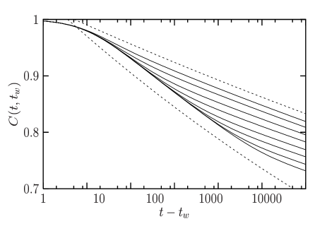
FIG. 1.: Analytical result (11) for the correlation functions for ordered initial conditions and different $t_{w}$. The dashed lines are power laws with exponents $-\eta/2$ (quasi-equilibrium part) and $-\eta/4$ (ageing part). We have chosen $a=1$, $\eta/2=0.03$, and $t_{w}=1,\,3,\,10,\cdots,\,3000$, from top to bottom.

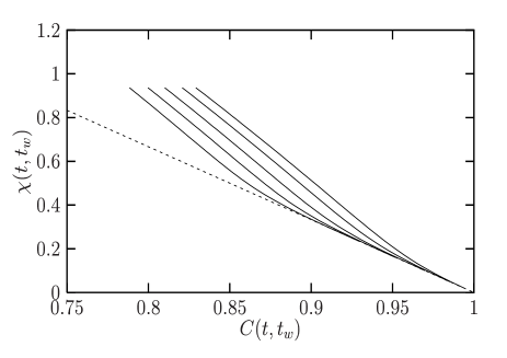
FIG. 2.: Analytical result for the parametric Susceptibility/Correlation plot, with $a=1$, $\eta/2=0.03$ and $t_{w}=1,\,3,\,10,\,30$ and 100, from top to bottom. The dashed line is the equilibrium FDT between $\chi$ and $C$.

This scaling is in complete agreement with the results obtained by Godrèche and Luck [12] for the spherical model at the critical point. Its physical interpretation is straightforward. At time $t_{w}$, fluctuations of wavelength smaller than $\xi(t_{w})$ have equilibrated, while others have not. The quasi-equilibrium regime corresponds then to equilibrium fluctuations of small wavelengths. At equilibrium, the correlation decays as $C_{\rm eq}(t)\sim t^{-2\beta/\nu z}$. For the 2D XY model [35], one has $\beta/\nu=\eta(T)/2$, $z=2$; hence the exponent describing the stationary regime of the correlation function is $-2\beta/\nu z=-\eta(T)/2$, as found in Eq. (17).

At the crossover time $t-t_{w}\sim t_{w}$, the autocorrelation has the value $C(t_{w}+t_{w},t_{w})\sim t_{w}^{-\eta(T)/2}$. It is interesting to compare this result with the case of ferromagnets quenched below $T_{c}$ where the crossover takes place for $C(t_{w}+t_{w},t_{w})\sim m_{\rm eq}(T)^{2}$. In this case the correlation function displays a plateau at the value $q_{EA}\equiv m_{\rm eq}(T)^{2}$, where $q_{EA}$ is the Edwards-Anderson parameter. There is then a clear time separation between the fast thermal fluctuations of very short wavelength (recall that $\xi_{\rm eq}(T)\ll t^{1/z}$) and the slow relaxation due to the domain wall motion. For $T=T_{c}$, there is no such distinction but only a ‘pseudo-plateau’ in the correlation, in the sense that the crossover takes place at a waiting time dependent value of the correlation. This reflects the fact that the order parameter vanishes in the thermodynamic limit.

The last regime, which takes place at a $t_{w}$-dependent time scale is the ageing regime. It is characterized by the loss of time-translation invariance and a breakdown of the FDT, $X(t,t_{w})\neq 1$. On this time scale, the decorrelation results from the growth of the correlation length. Note finally that although the response function is the product of a stationary and an ageing part, the latter is a very slowly varying function of the variable $t/t_{w}$. In a plot of $\chi(t,t_{w})$ vs $t-t_{w}$, there would be apparently no ageing in the response function.

For comparison with the numerical results of the full XY model, we show in Fig. 1 the analytical result (11) for the correlation functions, while in Fig. 2 we build the usual plot to study the FDT violations [3]. We have plotted the susceptibility $\chi(t,t_{w})\equiv\int_{t_{w}}^{t}{\mathrm{d}}t^{\prime}R(t,t^{\prime})$ as a function of $C(t,t_{w})$ parameterized by the time difference $t-t_{w}$, for different $t_{w}$. With the generalized form of the FDT, Eq. (1), the relation between $\chi$ and $C$ becomes

$$\chi(t,t_{w})= \frac{1}{T}\int_{t_{w}}^{t}{\mathrm{d}}t^{\prime}X(t,t^{\prime})\frac{\partial C(t,t^{\prime})}{\partial t^{\prime}}$$ (19)

$$= \frac{1}{T}\int_{C(t,t_{w})}^{1}{\mathrm{d}}C^{\prime}x(C^{\prime}),$$

where the second line holds when the FDR becomes a function of $C$ only. In this last case, the parametric plot reaches a master curve $\tilde{\chi}(C)$ independent of $t_{w}$, whose derivative ${\mathrm{d}}\tilde{\chi}/{\mathrm{d}}C$ is given by $x(C)$. At equilibrium, $x=1$ and $\tilde{\chi}(C)=(1-C)/T$. When the FDR is not a single variable function, only the first line of Eq. (19) can be used and the FDR $X(t,t_{w})$ is not the slope of the parametric plot. It is clear from Eqs. (16) that this happens in the 2D XY model, and a master curve $\tilde{\chi}$ is not reached.

Finally, we comment on the rather peculiar fact that in the time regime $\lambda\gg 1$ the FDR is larger than 1, which means from Eq. (19) that the susceptibility is larger than its equilibrium value, as can be seen in Fig. 2. When the system is quenched, all degrees of freedom which were equilibrated at temperature $T=0$, fall out of equilibrium at time $t=0$. As $t$ increases, ‘fast’ degrees of freedom equilibrate, while the ‘slow’ ones are still out of equilibrium. According to the interpretation of the FDR as an effective temperature [36], $x>1$ means that the slow degrees of freedom are ‘quasi-equilibrated’ at a temperature $T_{\text{eff}}\equiv T/x<T$. Applied to a quench from a high temperature state, this reasoning implies a FDR smaller than one, and the recovery of the usual case $x<1$. This argument is only qualitative, since the interpretation of FDT violations in terms of an effective temperature relies on the existence of well separated time scales, each one associated with an effective temperature; here instead there is no clear distinction between ‘slow’ and ‘fast’ degrees of freedom, since there are fluctuations of every length scales, each having its own relaxation time.

III Ageing dynamics: Monte-Carlo Results

In this section we present the results of Monte-Carlo simulations for the full XY model which allows to go beyond the spin-wave approximation. We first consider a quench from a completely ordered initial condition to check the validity of the scalings obtained in the previous Section. Then we consider a quench from a random initial condition in order to see how the vortex contribution changes the dynamical scaling and the FDT violations.

A Model and details of the simulation

The two-dimensional XY model is defined by the Hamiltonian

$$H=-\sum_{\langle i,j\rangle}\boldsymbol{\phi}_{i}\cdot\boldsymbol{\phi}_{j},$$ (20)

where the sum runs over nearest neighbors of a square lattice of linear size $L$, and the spins $\{\boldsymbol{\phi}_{j},\,j=1,\,2,\dots,\,L^{2}\}$ are bidimensional vectors of unit length. Introducing angular variables through $\boldsymbol{\phi}_{j}\equiv\exp(i\theta_{j})$, the Hamiltonian becomes

$$H=-\sum_{\langle i,j\rangle}\cos(\theta_{i}-\theta_{j}).$$ (21)

The Kosterlitz-Thouless transition temperature is located at $T_{KT}\simeq 0.89$ [37]. The model (21) is simulated by the following Monte Carlo algorithm: the angular variable $\theta_{i}$ associated to a randomly chosen site $i$ is updated to a new value $\theta_{i}^{\prime}$ randomly chosen in the interval $[-\pi,\pi]$, with probability $p=\min\left\{1,e^{-\beta\Delta E}\right\}$, where $\Delta E$ is the energy variation between the two configurations. We present results for a system of linear size $L=512$. We carefully checked that we are in a regime with $\xi(t)\ll L$.

We shall be interested in the spin-spin autocorrelation function $C(t,t_{w})$ and in its conjugated integrated response function $\chi(t,t_{w})$. The former is easily computed from

$$C(t,t_{w})=\frac{1}{L^{2}}\sum_{i=1}^{L^{2}}\langle\cos(\theta_{i}(t)-\theta_{i}(t_{w}))\rangle,$$ (22)

where the brackets denote an average over the realizations of the thermal noise. The computation of the latter is standard [5]. At time $t_{w}$, a perturbation $\Delta H=-\sum_{i}\boldsymbol{h}_{i}\cdot\boldsymbol{\phi}_{i}$ is added to the Hamiltonian. The magnetic field is random: its two components are independently drawn from a bimodal distribution $\pm h$. In the linear response regime, the integrated response function reads

$$\chi(t,t_{w})=\frac{1}{h^{2}\,L^{2}}\sum_{i=1}^{L^{2}}\overline{\langle\boldsymbol{h}_{i}\cdot\boldsymbol{\phi}_{i}\rangle},$$ (23)

where the overline means an average over the realizations of the random magnetic field. We checked that the value $h=0.04$ was small enough for the response to be linear.

B Ordered initial conditions

We investigate first the dynamic behaviour of the model (21) starting from a completely ordered initial condition. At $t=0$, the temperature is switched to $T<T_{KT}$. The evolution of the system may be followed in a series of snapshots in Fig. 3. At short times, the system is very ordered, and there is a single color in the first snapshot. As $t$ increases, fluctuations appear, and there is clearly a growing length scale in the system.

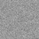
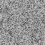
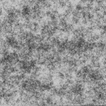
FIG. 3.: Snapshot of the domain growth in the XY model at $T=0.3$ for times $t_{w}=10^{2}$, $10^{3}$, $10^{4}$ and ordered initial conditions. The system size is $512\times 512$. The grey scale encodes the variable $\cos(\theta(\boldsymbol{x},t))$.

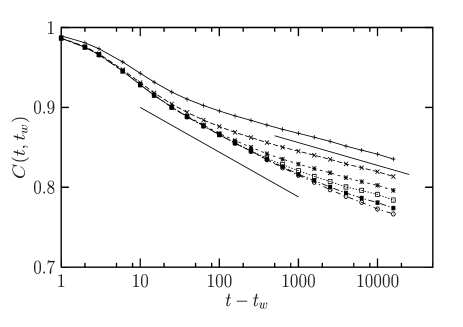
FIG. 4.: Autocorrelation function for ordered initial conditions, for waiting times $t_{w}=10$, 30, 100, 3000, 10000 (from top to bottom). The final temperature is $T=0.3$. The full lines are power laws with exponent $-\eta/2=-0.03$ and $-\eta/4=-0.015$.

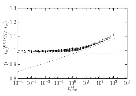
FIG. 5.: Rescaling of the autocorrelation functions of Fig. 4. The dashed lines are power laws with exponents 0 and 0.015. The rescaling is good, except for the smallest waiting time.

In Fig. 4, the autocorrelation $C(t,t_{w})$ is shown for the temperature $T=0.3$ and different waiting times $t_{w}$. The overall behaviour of $C(t,t_{w})$ is in nice agreement with the analytical results obtained in the spin-wave approximation, recall Fig. 1. As described in the previous section, there are two different regimes, depending on the time scale. For small time separation $t-t_{w}\ll t_{w}$, $C(t,t_{w})$ exhibits a stationary part, which is well represented by a power law

$$C(t,t_{w})\sim\frac{1}{(t-t_{w})^{0.03}},$$ (24)

while at long time, the different curves do not superpose: the system ages. We test the scaling (11) in Fig. 5, where we plot $(t-t_{w})^{0.03}C(t,t_{w})$ as a function of the scaling variable $t/t_{w}$. We have actually obtained the exponent 0.03 as the value insuring the best collapse of these data. This value of the exponent can be compared to the self-consistent computation of Ref. [35] which gives $\eta(T=0.3)\simeq 0.026$. It is in good agreement with its numerical estimation [37]. At $T=0.7$, we find $\eta/2=0.085$, in agreement with the numerical estimation of Ref. [37]; the self-consistent computation gives 0.069.

The parametric plot obtained numerically at $T=0.3$ for ordered initial conditions is represented in Fig. 6. It is also very similar to the analytical results of Fig. 2, confirming in particular the unusual feature of a FDR larger than 1.

The conclusion of the numerical study of ordered initial conditions is that the off-equilibrium dynamics is satisfactorily described by the spin-wave approximation. This is no longer true with random initial configurations on which we focus now.

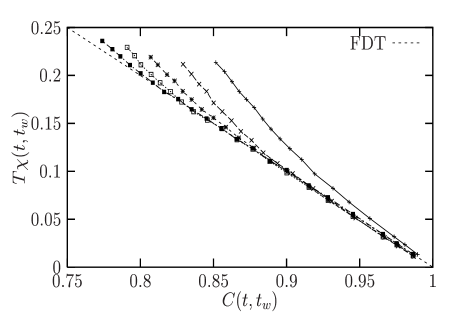
FIG. 6.: Parametric Susceptibility/Correlation plot for ordered initial conditions. The symbols are the same as in Fig. 4.

C Random initial conditions

The non-equilibrium dynamics for random initial conditions turns out to be quite different. However, our previous analytical results can be used to understand the scaling behaviour of the dynamic functions in that case too.

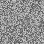
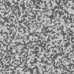
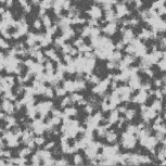
FIG. 7.: Snapshot of the domain growth in the XY model at $T=0.3$ for times $t_{w}=10$, $10^{2}$, $10^{3}$ and random initial conditions. The system size is $512\times 512$. The grey scale encodes the variable $\cos(\theta(\boldsymbol{x},t))$.

In Fig. 7 we present a series of snapshots for different times. A simple look at Figs. 7 and 3 makes the difference between the two situations very clear. The snapshots of Fig. 7 are moreover different from the ‘Schlieren patterns’ presented in $T=0$ simulations of the 2D XY model [27, 28, 31] and resulting from the presence of vortices. In the present work, vortices are also present, but they are blurred by thermal fluctuations, and do not clearly appear in the snapshots, except at $T$ close to zero.

In Fig. 8, we present the correlation function $C(t,t_{w})$ at $T=0.3$ and different waiting times $t_{w}$. The two distinct behaviours, namely a stationary part and an ageing part, are still present. The stationary part, corresponding to the equilibrium fluctuations, remains unchanged and can again be represented by the power law (24).

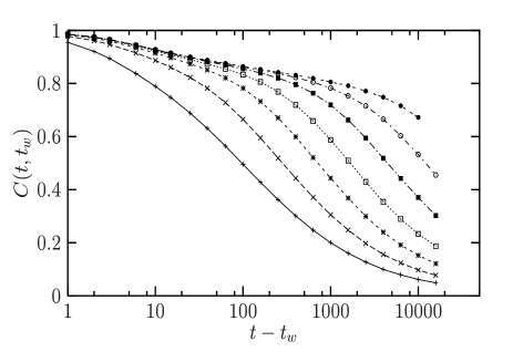
FIG. 8.: Correlation functions for random initial conditions at $T=0.3$ and waiting times $t_{w}=10$, 30, 100, 300, 1000, 3000 and 10000 from bottom to top.

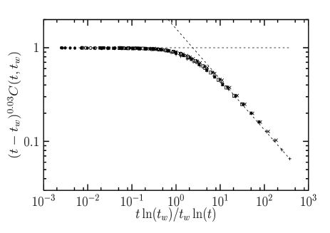
FIG. 9.: Rescaled correlation functions for random initial conditions at $T=0.3$; the data are the same as in Fig. 8. The two dashed lines are power laws with exponents 0 and -0.54.

The ageing part is different because of the presence of vortices in the system. By analogy with the previous case, we conjecture that $C(t,t_{w})$ has the scaling form

$$C(t,t_{w})=\frac{1}{(t-t_{w})^{\eta(T)/2}}\Phi\left(\frac{\xi(t)}{\xi(t_{w})}\right),$$ (25)

where $\Phi$ is a scaling function and $\xi(t)$ is the growing correlation length. Previous numerical and analytical studies have shown that an effect of the vortices is to change the growth law for the correlation length from the power law $\xi(t)\sim t^{1/z}$ to the form $\xi(t)\sim\sqrt{t/\ln t}$ [25, 27, 31]. The scaling prediction for $C(t,t_{w})$ is tested in Fig. 9 where we plot $(t-t_{w})^{0.03}C(t,t_{w})$ as a function of $\xi(t)/\xi(t_{w})$ including the logarithmic correction due to the vortices. The rescaling is very good. It is seen in particular that the long time decay is well described by a power law, i.e. $\Phi(x)\sim x^{-\lambda}$ for large $x$. At $T=0.3$, we find $\lambda=0.54$. An asymptotic power law behaviour was also found in Ref. [12] for the ferromagnetic spherical model.

It is also interesting to note that the $t/t_{w}$-scaling, usually called ‘simple ageing’ [1] and encountered for an ordered initial state, is changed to a ‘non-simple’ ageing with the scaling $t\ln t_{w}/t\ln t$ when topological defects (here vortices) are present. Although the two scalings are equivalent in the large waiting time limit, the latter is preasymptotically equivalent to a sub-ageing behaviour [38].

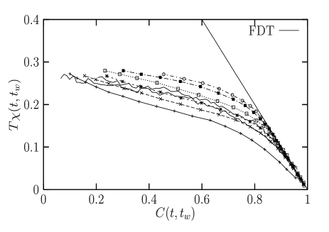
FIG. 10.: Parametric Susceptibility/correlation plot for $T=0.3$ and random initial conditions. The symbols are the same as in Fig. 8. The two full lines are similar data obtained with the 3D Edwards-Anderson model (see text).

We turn now to the FDT violations. We present in Fig. 10 the parametric plot Susceptibility/Correlation. There are still two distinct behaviours depending on the time scale. At short time separation FDT holds, whereas at long time separation a non-equilibrium regime is entered. This plot is very different from the one obtained in Fig. 2 for ordered initial conditions in the sense that the susceptibility is smaller than the value obtained from the FDT. In short, this means that $X(t,t_{w})<1$. In the qualitative picture developed above in terms of an effective temperature, this means that the fluctuations of wavelength larger than $\xi(t_{w})$ are ‘quasi-equilibrated’ at a temperature higher than the thermal bath temperature, keeping then the memory of their $T=\infty$ initial state.

It is interesting to note the close similarity of this plot with those observed in simulations of the 3D Edwards-Anderson model [8, 39, 40]. We have superposed as continuous lines the data obtained in Ref. [40].

IV The link between statics and dynamics

In this Section we compute the finite-size Parisi function and compare it with the finite-time fluctuation-dissipation ratio obtained in the previous Section.

A The Parisi function in the finite-size 2D XY model

In order to compute the Parisi function $P(q,L)$ for the 2D XY model, one has to carefully define the overlap $q$. Two different overlaps between configurations (1) and (2) may be defined, namely

$$q^{12}=\frac{1}{L^{2}}\sum_{i=1}^{L^{2}}\cos[\theta_{i}^{1}-\theta_{i}^{2}]$$ (26)

or

$$\tilde{q}^{12}=\frac{1}{L^{2}}\sum_{i=1}^{L^{2}}\cos[\theta_{i}^{1}-\psi^{1}-\theta_{i}^{2}+\psi^{2}],$$ (27)

where $\psi^{a}=N^{-1}\sum_{i}\theta_{i}^{a}$. According to the prescription of Ref. [6], the $O(2)$ symmetry of the Hamiltonian has to be taken into account. We have therefore considered the first definition. The Parisi function $P(q,L)$ can be related to the probability distribution function of the magnetization $Q(m,L)$, where

$$m=\frac{1}{N}\sum_{i=1}^{N}\cos[\theta_{i}-\psi]\,.$$ (28)

The function $Q(m,L)$ gives the magnetization fluctuations in the direction defined by the mean orientation $\psi$, which contains the physics of the critical fluctuations [23]. It has been analytically computed in Refs. [23]. The two first moments $\langle m\rangle$ and $\sigma=\sqrt{\langle m^{2}\rangle}$ of the distribution scale as [34]

$$\langle m\rangle\sim L^{-\eta(T)/2},\quad\sigma\sim T\langle m\rangle\,.$$ (29)

The temperature and size dependence of the distribution enters only these two moments, and $Q(m,L)$ takes the scaling form [23, 34]

$$Q(m,L)=\sigma^{-1}\,{\cal F}\left(\frac{m-\langle m\rangle}{\sigma}\right),$$ (30)

where ${\cal F}(x)$ is a scaling function whose functional from is well approximated by a generalized Gumbel distribution [23]:

$${\cal F}(x)=K(e^{y-e^{y}})^{\pi/2},\quad y=b(x-s),$$ (31)

where $K$, $b$ and $s$ are numerical constants ensuring the normalization of the distribution.

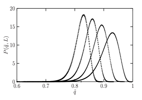
FIG. 11.: The Parisi function $P(\tilde{q},L)$ for the 2D XY model at $T=0.3$ and system sizes $L=4$, 8, 16, 32 from right to left.

From $Q(m,L)$, it is easy to obtain the critical fluctuations of the overlap in the direction defined by the mean angle $\psi$, i.e. using the definition (27), by the relation

$$P(\tilde{q},L)=\frac{1}{2\sqrt{\tilde{q}}}Q(\sqrt{\tilde{q}},L).$$ (32)

This function is displayed in Fig. 11 for different system sizes. Its scaling properties follow from those of $Q(m,L)$ [23, 34] and are typical of the fluctuations of the order parameter at a critical point [18]. The mean values scale with system size as $\langle\tilde{q}\rangle\sim L^{-2\beta/\nu}$, as do the widths of the curves. This result is expected from the hyperscaling relation between critical exponents and is compatible with a diverging susceptibility. However it is not sufficient to give a finite amplitude for the probability at $\tilde{q}=0$. As could be estimated from Fig. 11, the probability function has an exponential tail for $q$ values below the mean, leading to much larger fluctuations than for a Gaussian function, but the tail of the distribution is still immeasurably small at $\tilde{q}=0$.

When the definition (26) of the overlap is used, a finite probability is generated at $q=0$ and a distribution reminiscent of the Parisi function for spin glasses is obtained [20]. In this case the $O(2)$ symmetry is included and $P(q,L)$ takes account of the fact that the magnetization vector diffuses around the perimeter of a circle. It is obtained from $Q(m,L)$ by the relation

$$P(q,L)=\frac{2}{\pi}\int_{\sqrt{q}}^{1}{\mathrm{d}}m\frac{Q(m,L)}{\sqrt{m^{4}-q^{2}}}.$$ (33)

The result is shown in Fig. 12 for different system sizes. That the tail is the product of this diffusive motion and is not the result of critical fluctuations can be seen by considering the overlap between two rigid rotors of unit length diffusing on a circle, for which $q=|\cos\theta|,\;\;q\geq 0$ and where $\theta$ is the angle between the two rod directions: this amounts to computing $P(q,L)$ at $T=0$. In this case, $P(q,L)$ is proportional to the density of states of $\cos\theta$ on the circle and it follows easily that

$$P(q,L)={2\over{\pi}}{1\over{\sqrt{1-q^{2}}}}.$$ (34)

The intercept at $q=0$ in Fig. 12 is quite close to the above value of $2/\pi\simeq 0.64$, while the essential singularity at $q=1$ is removed by the fluctuations in length of the magnetization vector. The critical behaviour manifests itself again in the width and position of the maximum probability, which scale with system size as in Fig. 11. Apart from this scaling of the peak, one would expect the same qualitative behaviour for the low temperature phase of the 3D XY or 4D XY models, where symmetry is broken in the thermodynamic limit.

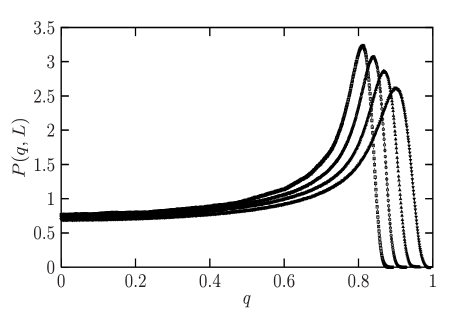
FIG. 12.: The Parisi function $P(q,L)$ for the 2D XY model at $T=0.3$ and system sizes $L=4$, 8, 16, 32 from right to left.

While this explanation of the tail in $P(q,L)$ seems rather trivial it is perhaps worth pointing out that the breaking of symmetry in an XY model provides a very simple analog for the breaking of replica symmetry in a mean field spin glass: the XY magnet contains an infinity of pure states $\alpha$ which are the points on the circle. On heating and cooling in zero field the system samples different points on the circle. It is true that these pure states are connected by a line of constant free energy around the circle and so in principle the system can change pure states without jumping free-energy barriers. However, symmetry breaking means that the diffusion constant around the circle goes to zero in the thermodynamic limit and the system never leaves its chosen pure state. Moving from one pure state to another across the circle does involve jumping a free-energy barrier in complete analogy with the spin glass. The overlap function between the pure ground states of the XY ferromagnet is therefore given by the expression (34) above. We note finally that distances between pure states of the 2D XY model on the circle do not verify the ultrametric inequality [41], and hence are not organized in the hierarchical way they are in a mean-field spin glass.

B Finite-size statics vs finite-time dynamics

We are now in position to test the relation (3) presented in the Introduction. We compare the dynamic parametric plot Susceptibility/Correlation (data of Fig. 10) at two different temperatures, $T=0.7$ and $T=0.3$, with the curves obtained through the relation (3).

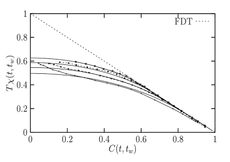
FIG. 13.: Comparison between the dynamical data and the curves built from the Parisi functions using the conjecture (3) at $T=0.7$. The linespoints are the dynamical data, while the full lines are the static data.

At $T=0.7$, we find an excellent agreement between the dynamic and static data (see Fig. 13). This strongly supports our conjecture that the dynamic behaviour can be described in terms of the static distribution of a finite-size system of linear dimension such that $L=\xi(t_{w})$. There is a small systematic deviation between the two sets of curves on the left hand side of the parametric plot. This corresponds to the limit where the total simulation time is a lot greater than $t_{w}$, which is most easily seen when $t_{w}$ is small. In the regime where $C(t,t_{w})$ is small and hence $\xi(t)\gg\xi(t_{w})$, one can no longer expect the relation (3) to be satisfied.

At much lower temperature $T=0.3$, the two sets of curve coincide in the quasi-equilibrium regime $C>q_{EA}$ and the departure point from the FDT is correctly predicted by the static data (see Fig. 14). As discussed above, this breaking point is given by $C(t_{w}+t_{w},t_{w})\sim t_{w}^{-\eta(T)/2}$, which coincides with the peak in the Parisi function $\langle q\rangle=L^{-2\beta/\nu}$, with $L=t_{w}^{1/z}$. Although the qualitative shape of the curves in the ageing regime is the same for the two sets, there is a quantitative discrepancy. This suggest that, while Eq. (3) is a correct starting point, the analytic $P(q,L)$ that we have calculated is not in this case quantitatively accurate.

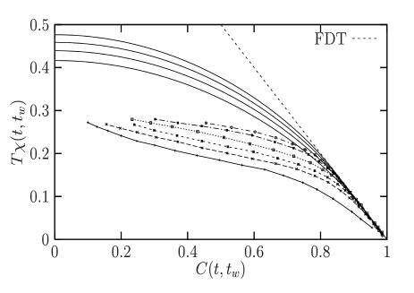
FIG. 14.: Comparison between the dynamical data and the curves built from the Parisi functions using the conjecture (3) at $T=0.3$. The linespoints are the dynamical data, while the full lines are the static data.

Indeed, in deriving this function we have explicitly neglected vortices which play a crucial role in the transition from order to disorder in the 2D XY model [19]. Since vortices are present during the coarsening process, one should consider their contribution to the static fluctuations. We do not know precisely how this has to be done, for instance we do not know what density and what vortex correlation to introduce. However, it is clear that the presence of defects can dramatically alter the shape of the function $P(q,L)$. As an illustration, we have calculated numerically $P(q,L)$ in the presence of a pinned defect. We have slaved a single spin in the opposite direction to its left neighbour and found that the tail at small $q$ is considerably reduced.

As a first step in investigating the effect of vortices, we show in Fig. 15 vortex configurations at the same waiting time, $t_{w}=10^{3}$, for $T=0.3$ and $T=0.7$. While the number of vortices is of the same order (474 for $T=0.3$ and 602 for $T=0.7$), their correlations are clearly different. At low temperature, the vortices of opposite charge are essentially uncorrelated, while at higher temperature, the majority of vortices are in closely bound pairs. This is because the diffusion of vortices is more efficient at higher temperature and so their natural tendency to form pairs is largely satisfied. The effect of a free vortex in the system is much more dramatic than a vortex pair [19]. In Fig. 15, there are far more free vortices at the lower temperature and hence one can expect that the static analysis in the absence of vortices describes more accurately the situation at $T=0.7$ than at $T=0.3$. This is consistent with our observations in Figs. 13 and 14.

FIG. 15.: Vortex configurations at time $t_{w}=10^{3}$ after a quench from a random initial condition to a temperature $T=0.3$ (above) and $T=0.7$ (below). Antivortices are represented by squares, vortices by plus symbols.

V Discussion

We have studied in this work the nonequilibrium critical dynamics of the 2D XY model and its relation with static properties. We have investigated the ageing behaviour of the system by looking at two-time dynamical functions and by considering quenches from random and ordered initial states to temperatures below the Kosterlitz-Thouless transition. We have then shown that the finite-time violations of the FDT are related to the finite-size equilibrium Parisi function. We discuss now some consequences of our results.

A first important feature is the scaling (25) of the spin-spin autocorrelation function. Figure 8 shows that the behaviour of $C(t,t_{w})$ is, at first sight, very similar to the usual additive decomposition between a stationary and an ageing part [1]. We have seen that, at a critical point, this decomposition is instead multiplicative. Interestingly, the same scaling is observed in numerical simulations of the 3D Edwards-Anderson model [42, 43]. It is indeed notoriously difficult to obtain the value of the Edwards-Anderson parameter $q_{EA}$, the plateau in the correlation function, in 3D Ising spin glasses [42]. This similarity means that the dynamics of 3D spin glasses is influenced, at least at short time, by the presence of a critical point.

This multiplicative decomposition has also consequences in the scaling behaviour of the response function. In the case of a quench in a ferromagnetic phase, the susceptibility $\chi(t,t_{w})$ can be decomposed into a ‘bulk’ and an ‘interface’ contribution [5]. The bulk contribution accounts for the equilibrium fluctuations inside the domains, while the interface contribution accounts for the domain wall response. Since their density vanishes at long time, so does their response function. This is not true at the critical point, where there are no clearly well defined ‘domains’: on a length scale $\xi(t)$, the ‘bulk’ is composed of critical fluctuations, a self-similar structure composed of domains within domains [14, 15, 18]. The direct consequence is that in a parametric Susceptibility/Correlation plot, no master curve $\tilde{\chi}(C)$ (as predicted by the dynamical mean-field theory) can ever be reached. The difference is irrelevant for the Ising spin chain at $T=0$, since there is no stationary part at all [12, 13].

We have conjectured a finite-time, finite-size generalization of the relation (2) in Eq. (3) and shown that it works in the present model provided that the temperature is not very low. We wish to mention that the conjecture (3) has been implicitly used by Marinari et al. in Ref. [8]. These authors have indeed shown that dynamic and static data for a 3D spin glass perfectly overlap, using the relation (3) with $t_{w}=10^{5}$ and $L=16$. Since $P(q,L)$ still depends on the size $L$ for $L=16$, and the $\chi$ vs $C$ plot still depends on $t_{w}$ at $t_{w}=10^{5}$ (because of the scaling (25)), the coincidence of the two sets of curves necessarily results from Eq. (3). It is interesting to note that this correspondance provides a direct measure of the dynamic correlation length $\xi(t)$.

As the temperature decreases, the agreement between the static and dynamic data is not as good because the density of free vortices increases. This is consistent with the results for the Ising chain at $T=0$ [13], where Eq. (2) has been used to deduce from the dynamic FDT violations a static ‘Parisi function’. The latter is not linked to the $T=0$ fluctuations of the spin glass order parameter which are trivial [44]. Rather, the dynamic behaviour has been shown to be entirely controlled by the domain walls. It would be interesting to see if a similar feature occurs at low temperature in the 3D Edwards-Anderson model.

Since the ageing dynamics of the 2D XY model closely resembles that of more complex systems, it is important to understand why this is so. We believe that the main ingredient for this behaviour is the presence of the critical fluctuations. After a quench, magnetic fluctuations of wave vectors between $k\sim 1/a$ and $k\sim 1/L$ try to develop in a system of size $L$ and lattice spacing $a$. At time $t_{w}$, only the fluctuations with $k\gtrsim t_{w}^{-1/z}$ are equilibrated, while those with $k\lesssim t_{w}^{-1/z}$ are out of equilibrium, the smallest $k$ being very far away from the equilibrium. As a result, the decay of the autocorrelation function is dictated by the growth of the correlation length which gives the $\xi(t)/\xi(t_{w})$-scaling of Eq. (25). Hence, this decay takes place in a single time scale. However, the coexistence of multiple length scales, each having its own relaxation time, implies FDT violations described by the smooth parametric plots of Fig. 10. The coexistence of a single time scale in the ageing regime together with a smooth $\chi$ vs $C$ plot arises naturally within this critical scenario. This feature, observed in 3D and 4D spin glasses  [8, 39, 42, 43], has no interpretation within the mean-field dynamical theory, where multiple effective temperatures are necessarily associated with multiple time scales [1, 3, 4, 40].

The relevance of multiple length scales in the ageing dynamics of spin glasses has been emphasized by Bouchaud [45]. The example of the 2D XY model has shown that these length scales account well for the scaling properties of two-time dynamical functions and FDT violations. However, a necessary ingredient to explain more refined experimental results, such as the ‘rejuvenation and memory’ effects [46], lies in the role played by the temperature [45]. In this picture, based on the behaviour of elastic objects pinned by disorder, the relaxation time $t(\ell)$ associated with a length scale $\ell$ scales as $t(\ell)\propto\exp\left[\Upsilon(T)\ell^{\theta}/T\right]$, in the notations of Ref. [45]. In the case of the 2D XY model the scaling is instead $t(\ell)\sim\ell^{z}$, independently of the temperature $T$. This means that such a model will not be able to capture subtle temperature-cycling effects. In this respect, it would be interesting to combine the modified domain growth approach recently proposed by Yoshino et al. [47] with nonequilibrium critical dynamics.

REFERENCES

- [1] J.-P. Bouchaud, L. F. Cugliandolo, J. Kurchan and M. Mézard in Spin Glasses and Random Fields, Ed.: A. P. Young (World Scientific, Singapore, 1998).
- [2] L. F. Cugliandolo and J. Kurchan, Phys. Rev. Lett. 71, 173 (1993).
- [3] L. F. Cugliandolo and J. Kurchan, J. Phys. A 27 (1994) 5749; Philos. Mag. B 71, 501 (1995).
- [4] S. Franz and M. Mézard, Europhys. Lett. 26, 209 (1994); Physica A 210, 48 (1994).
- [5] A. Barrat, Phys. Rev. E 57, 3629 (1998); L. Berthier, J.-L. Barrat and J. Kurchan, Eur. Phys. J. B 11, 635 (1999); L. F. Cugliandolo and D. S. Dean, J. Phys. A 28, 4213 (1995); S. A. Cannas, D. A. Stariolo and F. A. Tamarit, preprint cond-mat/0010319; L. Berthier, Eur. Phys. J. B 17, 689 (2000). D. A. Stariolo and S. A. Cannas, Phys. Rev. B 60, 3013 (1999); G. Parisi, F. Ricci-Tersenghi and J. J. Ruiz-Lorenzo, Eur. Phys. J. B 11, 317 (1999).
- [6] S. Franz, M. Mézard, G. Parisi and L. Peliti, Phys. Rev. Lett. 81, 1758 (1998); J. Stat. Phys. 97, 459 (1999).
- [7] G. Parisi, Phys. Rev. Lett. 50, 1946 (1983).
- [8] E. Marinari, G. Parisi, F. Ricci-Tersenghi and J. J. Ruiz-Lorenzo, J. Phys. A 31, 2611 (1998).
- [9] J. Zarzicki, Glasses and th Vitreous State (Cambridge University Press, Cambridge, 1991).
- [10] L. C. E. Struik, Physical Aging in Amorphous Polymers and Other materials, (Elsevier, Houston, 1978).
- [11] M. Sellitto, Eur. Phys. J. B 4, 135 (1998).
- [12] C. Godrèche and J.M. Luck, J. Phys. A: Math. Gen. 33, 1151 (2000); J. Phys. A: Math. Gen. 33, 9141 (2000).
- [13] E. Lippiello and M. Zannetti, Phys. Rev. E 61, 3369 (2000); F. Corberi, E. Lippiello and M. Zannetti, preprint cond-mat/0007021.
- [14] P. C. Hohenberg and B. I. Halperin, Rev. Mod. Phys. 49, 435 (1977).
- [15] S. K. Ma, Modern Theory of Critical phenomena, (Benjamin, New York, 1976).
- [16] H. K. Janssen, B. Schaub and B. Schmittmann, Z. Phys. B 73, 539 (1989).
- [17] A. J. Bray, Adv. Phys. 43, 357 (1994).
- [18] K. Binder in Computational Methods in Field Theory, Eds.: H. Gauslever and C. B. Lang (Springer-Verlag, Berlin, 1992); K. Binder, Z. Phys. B 43, 119 (1981).
- [19] J. M. Kosterlitz and D. J. Thouless, J. Phys. C 6, 1181 (1973).
- [20] D. Iñiguez, E. Marinari, G. Parisi and J. J. Ruiz-Lorenzo, J. Phys. A: Math. Gen. 30, 7337 (1997).
- [21] J.-P. Bouchaud and M. Mézard, J. Phys. A 30, 7997 (1997).
- [22] S.T. Bramwell, K. Christensen, J.-Y. Fortin, P.C.W. Holdsworth, H.J. Jensen, S. Lise, J. López, M. Nicodemi, J.-F. Pinton, and M. Sellitto, Phys. Rev. Lett. 84, 3744 (2000).
- [23] S.T. Bramwell, J.-Y. Fortin, P.C.W. Holdsworth, S. Peysson, B. Portelli, J.-F. Pinton, and M. Sellitto, preprint cond-mat/0008093, to appear in Phys. Rev. E (March 2001).
- [24] S.T. Bramwell, P.C.W. Holdsworth and J.-F. Pinton, Nature 396 552 (1998).
- [25] A. J. Bray, A. J. Briant and D. K. Jervis, Phys. Rev. Lett. 84, 1503 (2000); A. J. Bray, Phys. Rev. E 62, 103 (2000).
- [26] A. D. Rutenberg and A. J. Bray, Phys. Rev. E 51, R1641 (1995).
- [27] F. Rojas and A. D. Rutenberg, Phys. Rev. E 60, 212 (1999).
- [28] X. Leoncini, A.D. Verga and S. Ruffo, Phys. Rev. E 57, 6377 (1998).
- [29] M. Mondello and N. Goldenfeld, Phys. Rev. A 42, 5865 (1990).
- [30] J.-R. Lee, S. J. Lee and B. Kim, Phys. Rev. E, 52, 1550 (1995).
- [31] B. Yurke, A. N. Pargellis, T. Kovacs and D. A. Huse, Phys. Rev. E 47, 1525 (1993).
- [32] G. F. Mazenko and R. A. Wickham, Phys. Rev. E 57, 2539 (1998); Phys. Rev. E 55, 5113 (1997).
- [33] L. F. Cugliandolo, J. Kurchan and G. Parisi, J. Phys. I (France) 4, 1641 (1994).
- [34] P. Archambault, S. T. Bramwell and P. C. W. Holdsworth, J. Phys. A: Math. Gen. 30, 8363 (1997).
- [35] V. L. Pokrovsky and G. V. Uimin, Phys. Lett. A 45, 467 (1973).
- [36] L. F. Cugliandolo, J. Kurchan and L. Peliti, Phys. Rev. E 55, 3898 (1997).
- [37] R. Gupta and C. F. Baillie, Phys. Rev. B 45, 2883 (1992).
- [38] É. Vincent, J. Hammann, M. Ocio, J.-Ph. Bouchaud and L. F. Cugliandolo, in Complex behaviour of glassy systems, Ed.: M. Rubi (Springer Verlag, Berlin, 1997). P. Nordblad and P. Svendlidh in Spin Glasses and Random Fields, Ed.: A. P. Young (World Scientific, Singapore, 1998).
- [39] J.-O. Andersson, J. Mattsson and P. Svedlindh, Phys. Rev. B 46, 8297 (1992); S. Franz and H. Rieger, J. Stat. Phys. 79, 749 (1995); E. Marinari, G. Parisi, F. Ricci-Tersenghi and J. J. Ruiz-Lorenzo, J. Phys. A 33, 2373 (2000).
- [40] L. Berthier, J.-L. Barrat and J. Kurchan, Phys. Rev. E 63, 0106105 (2001).
- [41] M. Mézard, G. Parisi and M. A. Virasoro, Spin Glass Theory and Beyond (World Scientific, Singapore, 1987).
- [42] E. Marinari, G. Parisi and J. J. Ruiz-Lorenzo in Spin Glasses and Random Fields, Ed.: A.P. Young (World Scientific, Singapore, 1998).
- [43] J. Kisker, L. Santen, M. Schreckenberg and H. Rieger, Phys. Rev. B 53, 6418 (1996).
- [44] The probability distribution of the magnetization may be easily computed through recursive methods, see R. Mélin, Ann. Phys. Fr. 22, 233 (1997); R. Mélin, J. C. Anglès d’Auriac, P. Chandra and B. Douçot, J. Phys. A 29 5773 (1996).
- [45] J.-P. Bouchaud in Soft and fragile matter, nonequilibrium dynamics, metastability and flow, Ed.: M. E. Cates and M. R. Evans (Institute of Physics Publishing, Bristol, 2000); preprint cond-mat/9910387.
- [46] K. Jonason, É. Vincent, J. Hammann, J.-P. Bouchaud and P. Nordblad, Phys. Rev. Lett. 81, 3243 (1998).
- [47] H. Yoshino, A. Lemaître and J.-P. Bouchaud, preprint cond-mat/0009152.