Degree Distributions of Growing Networks

Abstract

The in-degree and out-degree distributions of a growing network model are determined. The in-degree is the number of incoming links to a given node (and vice versa for out-degree). The network is built by (i) creation of new nodes which each immediately attach to a pre-existing node, and (ii) creation of new links between pre-existing nodes. This process naturally generates correlated in- and out-degree distributions. When the node and link creation rates are linear functions of node degree, these distributions exhibit distinct power-law forms. By tuning the parameters in these rates to reasonable values, exponents which agree with those of the web graph are obtained.

PACS numbers: 02.50.Cw, 05.40.-a, 05.50.+q, 87.18.Sn

The world-wide web (WWW) is a rapidly evolving network which now contains nearly $10^{9}$ nodes. Much recent effort has been devoted to characterizing the underlying directed graph formed by these nodes and their connecting hyperlinks – the so-called “web” graph[1, 2, 3, 4]. In parallel with these developments, a variety of growing network models have recently been introduced and studied[5, 6, 7, 8, 9, 10, 11, 12, 13, 14]. These model networks are built by sequentially adding both nodes and links in a manner which mimics the evolution of real network systems, with the WWW being the most obvious example.

One fundamental characteristic of any graph is the number of links at a node – the node degree. The growing network models cited above predict that the distribution of node degree has a power law form for growth rules in which the probability that a newly-created node attaches to a pre-existing node increases linearly with the degree of the “target” node[5, 6, 7, 8]. This power law behavior strongly contrasts with the Poisson degree distribution of the classical random graphs[15], where links are randomly created between any pair of pre-existing nodes in the network.

FIG. 1.: A node with in-degree $i=4$, out-degree $j=5$, and total degree 9.

Since web links are directed, the total degree of a node may naturally be resolved into the in-degree – the number of incoming links to a node, and out-degree – the number of outgoing links from a node (Fig. 1). While the total node degree and its distribution are now reasonably understood [5, 6, 7, 8, 11], little is known about the joint distribution of in-degrees and out-degrees, as well as their correlation. Empirical measurements of the web indicate that in-degree and out-degree distributions exhibit power-law behaviors with different exponents[2, 3, 4]. In this Letter, we solve for the joint distribution in a simple growing network model. We are able to reproduce the observed in-degree and out-degree distributions of the web as well as find correlations between in- and out-degrees of each node.

Our model represents an extension of growing network models with node and link creation[13, 14] to incorporate link directionality. The network growth occurs by two distinct processes (Fig. 2):

• With probability $p$, a new node is introduced and it immediately attaches to one of the earlier target nodes in the network. The attachment probability depends only on the in-degree of the target.

• With probability $q=1-p$, a new link is created between already existing nodes. The choices of the originating and target nodes depend on the out-degree of the originating node and the in-degree of the target node.

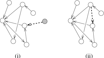
FIG. 2.: Illustration of the growth processes in the growing network model: (i) node creation and immediate attachment, and (ii) link creation. In (i) the new node is shaded, while in both (i) and (ii) the new link is dashed.

If only process (i) was allowed, the out-degree of each node would be one by construction. Process (ii) has been shown to drive a transition in the network structure[14]. We shall further show that this general model gives a non-trivial out-degree distribution which is distinct from the in-degree distribution.

We begin our analysis by determining the average node degree; this can be done without specification of the attachment and link creation probabilities. Let $N(t)$ be the total number of nodes in the network, and let $I(t)$ and $J(t)$ be the total in-degree and out-degree, respectively. According to the two basic growth processes enumerated above, at each time step these degrees evolve according to one of the following two possibilities

$$(N,I,J)\to\cases{(N+1,I+1,J+1)&probability $p$,\cr(N,I+1,J+1)&probability $q$.}$$ (1)

That is, with probability $p$ a new node and new directed link are created (Fig. 2) so that the number of nodes and both node degrees increase by one. Conversely, with probability $q$ a new directed link is created and the node degrees each increase by one, while the total number of nodes is unchanged. As a result,

$$N(t)=pt,\qquad I(t)=J(t)=t,$$ (2)

from which we immediately conclude that the average in- and out-degrees, ${\cal D}_{\rm in}\equiv I(t)/N(t)$ and ${\cal D}_{\rm out}\equiv J(t)/N(t)$, are both time independent and equal to $1/p$.

To determine the joint degree distributions, we need to specify: (i) the attachment rate $A(i,j)$, defined as the probability that a newly-introduced node links to an existing node with $i$ incoming and $j$ outgoing links, and (ii) the creation rate $C(i_{1},j_{1}|i_{2},j_{2})$, defined as the probability of adding a new link from a $(i_{1},j_{1})$ node to a $(i_{2},j_{2})$ node. We restrict the form of these rates to those which we naturally expect to occur in systems such as the web graph. First, we assume that the attachment rate depends only on the in-degree of the target node, $A(i,j)=A_{i}$. We also assume that the link creation rate depends only on the out-degree of the node from which it emanates and the in-degree of the target node, that is, $C(i_{1},j_{1}|i_{2},j_{2})=C(j_{1},i_{2})$.

On general grounds, the attachment and creation rates $A_{i}$ and $C(j,i)$ should be non-decreasing functions of $i$ and $j$. For example, a web-page designer is more likely to construct hyperlinks to well-known pages rather than to obscure pages. Similarly, a web page with many outgoing hyperlinks is more likely to create even more hyperlinks. We have found that the degree distributions exhibit qualitatively different behaviors depending on whether the asymptotic dependence of the rates $A_{i}$ and $C(j,i)$ on both $i$ and $j$ grow slower than linearly, linearly, or faster than linearly. The first and last cases lead to either rapidly decaying degree distributions or to the dominance of a single node; this same behavior was already found for the total node degree[7, 11]. The most interesting behavior arises for asymptotically linear rates, and we focus on this class of models in our investigations.

Specifically, we consider the model with attachment and creation rates which are shifted linear functions in all indices (linear-bilinear rates)

$$A_{i}=i+\lambda,\qquad C(j,i)=(i+\lambda)(j+\mu).$$ (3)

An intuitively natural feature of this model is that both the attachment and creation rates have the same dependence on the popularity of the target node. The parameters $\lambda$ and $\mu$ in the rates of Eq. (3) must obey the constraints $\lambda>0$ and $\mu>-1$ to ensure that the corresponding rates are positive for all permissible values of in- and out-degrees, $i\geq 0$ and $j\geq 1$.

As the network grows, the joint degree distribution, $N_{ij}(t)$, defined as the average number of nodes with $i$ incoming and $j$ outgoing links, builds up. To solve for $N_{ij}(t)$, we shall use the rate equation approach, which has recently been applied to simpler versions of growing networks[7, 8, 11]. When the attachment and creation rates are given by Eq. (3), the degree distribution $N_{ij}(t)$ evolves according to the rate equations

$${dN_{ij}\over dt} = (p+q)\left[{(i-1+\lambda)N_{i-1,j}-(i+\lambda)N_{ij}\over I+\lambda N}\right]$$ (4)

$$+ q\left[{(j-1+\mu)N_{i,j-1}-(j+\mu)N_{ij}\over J+\mu N}\right]+p\,\delta_{i0}\delta_{j1}.$$ (5)

The first group of terms on the right-hand side account for the changes in the in-degree of target nodes. These changes arise by simultaneous creation of a new node and link (with probability $p$) or by creation of a new link only (with probability $q$). For example, the creation of a link to a node with in-degree $i$ leads to a loss in the number of such nodes. This occurs with rate $(p+q)(i+\lambda)N_{ij}$, divided by the appropriate normalization factor $\sum_{i,j}(i+\lambda)N_{ij}=I+\lambda N$. The factor $p+q=1$ in Eq. (4) has been written to make explicit the two types of relevant processes. Similarly, the terms in the second group of terms accounts for changes in the out-degree. These occur due to the creation of new links between already existing nodes – hence the prefactor $q$. The last term accounts for the continuous introduction of new nodes with no incoming links and one outgoing link. As a useful self-consistency check, we can easily verify that the total number of nodes, $N=\sum_{i,j}N_{ij}$, obeys $\dot{N}=p$, in agreement with Eq. (2). In the same spirit, the total in- and out-degrees, $I=\sum_{i,j}iN_{ij}$ and $J=\sum_{i,j}jN_{ij}$, obey $\dot{I}=\dot{J}=1$.

By solving the first few of Eqs. (4), it is clear that the $N_{ij}$ grow linearly with time. Accordingly, we substitute $N_{ij}(t)=t\,n_{ij}$, as well as $N=pt$ and $I=J=t$, into Eqs. (4) to yield a recursion relation for $n_{ij}$. Using the shorthand notations,

$$a=q\,{1+p\lambda\over 1+p\mu}\quad{\rm and}\quad b=1+(1+p)\lambda,$$

the recursion relation for $n_{ij}$ simplifies to

$$[i+a(j+\mu)+b]n_{ij} = (i-1+\lambda)n_{i-1,j}$$ (6)

$$+ a(j-1+\mu)n_{i,j-1}$$ (7)

$$+ p(1+p\lambda)\delta_{i0}\delta_{j1}.$$ (8)

We first consider the in-degree and out-degree distributions, ${\cal I}_{i}(t)=\sum_{j}N_{ij}(t)$ and ${\cal O}_{j}(t)=\sum_{i}N_{ij}(t)$. Because of the linear time dependence of the nodes degrees, we write ${\cal I}_{i}(t)=t\,I_{i}$ and ${\cal O}_{j}(t)=t\,O_{j}$. The densities $I_{i}$ and $O_{j}$ satisfy

$$(i+b)I_{i} = (i-1+\lambda)I_{i-1}+p(1+p\lambda)\delta_{i0},$$ (9)

$$\left(j+{1\over q}+{\mu\over q}\right)O_{j} = (j-1+\mu)O_{j-1}+p{1+p\mu\over q}\delta_{j1},$$ (10)

respectively. The solution to these recursion formulae may be expressed in terms of the following ratios of gamma functions

$$I_{i}=I_{0}\,{\Gamma(i+\lambda)\,\Gamma(b+1)\over\Gamma(i+b+1)\,\Gamma(\lambda)},$$ (11)

with $I_{0}=p(1+p\lambda)/b$, and

$$O_{j}=O_{1}\,{\Gamma(j+\mu)\,\,\Gamma(2+q^{-1}+\mu q^{-1})\over\Gamma(j+1+q^{-1}+\mu q^{-1})\,\Gamma(1+\mu)},$$ (12)

with $O_{1}=p(1+p\mu)/(1+q+\mu)$.

From the asymptotics of the gamma function, the asymptotic behavior of the in- and out-degree distributions have the power law forms,

$$I_{i}\sim i^{-\nu_{\rm in}},\qquad\nu_{\rm in} = 2+p\lambda,$$ (13)

$$O_{j}\sim j^{-\nu_{\rm out}},\qquad\nu_{\rm out} = 1+q^{-1}+\mu pq^{-1}.$$ (14)

These exponents for the degree distributions constitute one of our primary results. Note that $\nu_{\rm in}$ depends on $\lambda$ (an in-degree feature) while $\nu_{\rm out}$ depends on $\mu$ (an out-degree feature). Notice also that both the exponents are greater than 2.

We can also solve the recursion relation (6) for $n_{ij}$ when $i$ or $j$ is small. For example, we can express $n_{i1}$ as the ratio of two gamma functions. Then we can express $n_{i2}$ as the sum of two such ratios, etc. While there appears to be no simple general expression for the joint distribution, we can extract the limiting behaviors of $n_{ij}$ when $i$ or $j$ is large. We find

$$n_{ij}\sim\cases{i^{-\xi_{\rm in}}\,j^{\mu},&$1\ll j\ll i$;\cr j^{-\xi_{\rm out}}\,i^{\lambda-1},&$1\ll i\ll j$;}$$ (15)

with

$$\xi_{\rm in} = \nu_{\rm in}+{q\over p}\,{(\nu_{\rm in}-1)(\nu_{\rm out}-2)\over\nu_{\rm out}-1}$$ (16)

$$\xi_{\rm out} = \nu_{\rm out}+{1\over p}\,{(\nu_{\rm out}-1)(\nu_{\rm in}-2)\over\nu_{\rm in}-1}.$$ (17)

Thus the in- and out-degrees of a node are correlated – otherwise, we would have $n_{ij}=I_{i}O_{j}\sim i^{-\nu_{\rm in}}j^{-\nu_{\rm out}}$. This correlation between node degrees is our second basic result.

The analytical form of the joint distribution greatly simplifies when $\nu_{\rm in}=\nu_{\rm out}$, corresponding to $a=1$ and $\mu+b=2\lambda$. In this region of the parameter space, the recursion relation (6) reduces to

$$(i+j+2\lambda)n_{ij} = (i-1+\lambda)n_{i-1,j}$$ (18)

$$+ (j-1+\mu)n_{i,j-1}$$ (19)

$$+ p(1+p\lambda)\delta_{i0}\delta_{j1}.$$ (20)

Equation (18) is simpler than the general recursion (6) since the node degrees $i$ and $j$ now appear with equal prefactors. This feature allows us to transform Eq. (18) into a constant-coefficient recursion relation. Indeed, the substitution

$$n_{ij}={\Gamma(i+\lambda)\,\Gamma(j+\mu)\over\Gamma(i+j+2\lambda+1)}\,\,m_{ij}$$ (21)

reduces (18) to

$$m_{ij}=m_{i-1,j}+m_{i,j-1}+\gamma\,\delta_{i0}\delta_{j1},$$ (22)

with $\gamma=p(1+p\lambda)\,{\Gamma(1+2\lambda)/(\Gamma(\lambda)\,\Gamma(\mu+1))}$. We solve Eq. (22) by the generating function technique. Multiplying Eq. (22) by $x^{i}y^{j}$ and summing over all $i\geq 0,j\geq 1$ yields

$${\mathcal{M}}(x,y)\equiv\sum_{i=0}^{\infty}\sum_{j=1}^{\infty}m_{ij}x^{i}y^{j}={\gamma y\over 1-x-y}.$$ (23)

Expanding this latter expression we obtain

$$m_{ij}=\gamma\,\,{\Gamma(i+j)\over\Gamma(i+1)\,\Gamma(j)}.$$ (24)

Combining Eqs. (21) and (24) gives the joint in- and out-degree distribution

$$n_{ij}=\gamma\,\,{\Gamma(i+\lambda)\,\Gamma(j+\mu)\,\Gamma(i+j)\over\Gamma(i+1)\,\Gamma(j)\,\Gamma(i+j+2\lambda+1)}.$$ (25)

In analogy to Eq. (15), this joint distribution reduces to

$$n_{ij}=\gamma\,{i^{\lambda-1}j^{\mu}\over(i+j)^{2\lambda+1}}.$$ (26)

in the limit $i\to\infty$ and $j\to\infty$.

Another manifestation of the correlation in the degree distribution becomes evident by fixing the in-degree $i$ and allowing the out-degree $j$ to vary. We find that $n_{ij}$ reaches a maximum value when $j=i\mu/[2+(1+p)\lambda]$ (here we consider large $i$ and assume that $\mu>0$). Correspondingly, the average out-degree always scales linearly with the in-degree, $\langle j\rangle=i(\mu+1)/[(1+p)\lambda]$ (here the coefficient is always positive). Thus popular nodes – those with large in-degree – also tend to have large out-degrees. A dual property also holds: Nodes with large out-degree – those where many links originate – also tend to be popular.

Let us now compare our predictions with empirical observations for the world-wide web. The relevant results for the node degrees are[4]

$$\nu_{\rm in}\approx 2.1,\quad\nu_{\rm out}\approx 2.7,\quad{\cal D}_{\rm in}={\cal D}_{\rm out}\approx 7.5,$$ (27)

Setting the observed value ${\cal D}_{\rm in}={\cal D}_{\rm out}=7.5$ to $p^{-1}$ (see the discussion following Eq. (2)) we see that the predictions (13)–(14) match the observed values of the in- and out-degree exponents when $\lambda=0.75$ and $\mu=3.55$, respectively. With these parameter values we also have $\xi_{\rm in}\approx 5.0$ and $\xi_{\rm out}\approx 3.9$. Empirical measurements of these exponents would provide a definitive test of our model.

We have also investigated a simplified model with node creation rate $A_{i}=i+\lambda$, as above, but with link creation rate $C(j,i)=j+\mu$, which does not depend on the popularity of the target node $i$ (linear-linear rates). For this model, the rate equations for the evolution of the number of nodes with degrees $(i,j)$ have a similar structure to Eqs. (4) and they can be solved by the same approach as that given for the network with linear-bilinear growth rates. We find that the in- and out-degree distributions again have power-law forms. Moreover, the out-degree exponent is still given by Eq. (13), while the value of the in-degree exponent is now $\nu_{\rm in}=1+\lambda+p^{-1}$. If we set $p^{-1}=7.5$ to reproduce the correct average degree of the web graph, we see that $\nu_{\rm in}$ must be larger than 8.5. Similarly the linear-linear model with $A_{i}=i+\lambda$ and $C(j,i)=i+\mu$ gives a power-law in-degree distribution but the exponential out-degree distribution $O_{j}=p^{2}q^{j-1}$. Therefore linear-linear rate models cannot match empirical observations from the web.

Parenthetically, we can also solve completely the growing network with both constant node creation rate and constant link creation rate, $A_{i}=1$ and $C(j,i)=1$. While not necessarily a realistic model, it provides a useful exactly solvable case. By following the basic steps of the rate equation approach, we find the joint distribution

$$n_{ij}={p^{2}q^{j-1}\over{2^{i+j}}}\,\,{\Gamma(i+j)\over\Gamma(i+1)\Gamma(j)},$$ (28)

from which we deduce the in- and out-degree distributions: $I_{i}=p^{2}/(1+p)^{i+1}$ and $O_{j}=p^{2}q^{j-1}$. Again, the in- and out-degrees of a node are correlated.

In summary, we have studied a growing network model which incorporates: (i) node creation and immediate attachment to a pre-existing node, and (ii) link creation between pre-existing nodes. The combination of these two processes naturally leads to non-trivial in-degree and out-degree distributions. We computed many structural properties of the resulting network by solving the rate equations for the evolution of the number of nodes with given in- and out-degree. For link attachment rate linear in the target node degree and also link creation rate linear in the degrees of the two end nodes, power-law in- and out-degree distributions are dynamically generated. By choosing the parameters of the growth rates in a natural manner these exponents can be brought into accord with recent measurements of the web. Within this class of models, the linear-bilinear growth rates appears to be a viable candidate for describing the link structure of the web graph. The model also predicts power-law behavior when e.g., the in-degree is fixed and the out-degree varies. Significant correlations between the in- and out-degrees of a node develop spontaneously, in agreement with everyday experience. Quantitative measurements of correlations in the web graph would test our model and help construct a more realistic model of the world-wide web.

We are grateful for financial support of this work from NSF grant DMR9978902 and ARO grant DAAD19-99-1-0173 (PLK and SR), and a grant from the EPSRC (GJR).

REFERENCES

- [1] B. A. Huberman, P. L. T. Pirolli, J. E. Pitkow, and R. Lukose, Science 280, 95 (1998); S. M. Maurer and B. A. Huberman, nlin.CD/0003041.
- [2] J. Kleinberg, R. Kumar, P. Raghavan, S. Rajagopalan, and A. Tomkins, in: Proceedings of the International Conference on Combinatorics and Computing, Lecture Notes in Computer Science, Vol. 1627 (Springer-Verlag, Berlin, 1999).
- [3] S. R. Kumar, P. Raghavan, S. Rajagopalan, and A. Tomkins, in: Proceedings of the 25th Very Large Databases Conference, Edinburgh, Scotland, 1999 (Morgan Kaufman, Orlando, FL, 1999).
- [4] A. Broder, R. Kumar, F. Maghoul, P. Raghavan, S. Rajagopalan, R. Stata, A. Tomkins, and J. Wiener, Computer Networks 33, 309 (2000).
- [5] A. L. Barabási and R. Albert, Science 286, 509 (1999).
- [6] S. N. Dorogovtsev and J. F. F. Mendes, Phys. Rev. E 62, 1842 (2000).
- [7] P. L. Krapivsky, S. Redner, and F. Leyvraz, Phys. Rev. Lett. 85, 4629 (2000).
- [8] S. N. Dorogovtsev, J. F. F. Mendes, and A. N. Samukhin, Phys. Rev. Lett. 85, 4633 (2000).
- [9] M. E. J. Newman, S. H. Strogatz, and D. J. Watts, cond-mat/0007235.
- [10] G. Bianconi and A. L. Barabási, cond-mat/0011029.
- [11] P. L. Krapivsky and S. Redner, Phys. Rev. E 63, xxxx (2001) [cond-mat/0011094].
- [12] B. Tadić, Physica A 293, 273 (2001).
- [13] The earliest network model was proposed by H. A. Simon, Biometrica 42, 425 (1955) to describe word frequency; see also S. Bornholdt and H. Ebel, cond-mat/0008465.
- [14] R. Albert and A.-L. Barabási, Phys. Rev. Lett. 85, 5234 (2000); S. N. Dorogovtsev and J. F. F. Mendes, Europhys. Lett. 52, 33 (2000).
- [15] B. Bollobás, Random Graphs (Academic Press, London, 1985); S. Janson, T. Luczak, and A. Rucinski, Random Graphs (Wiley, New York, 2000).