[

Rapid algorithm for identifying backbones in the two-dimensional percolation model

Abstract

We present a rapid algorithm for identifying the current-carrying backbone in the percolation model. It applies to general two-dimensional graphs with open boundary conditions. Complemented by the modified Hoshen-Kopelman cluster labeling algorithm, our algorithm identifies dangling parts using their local properties. For planar graphs, it finds the backbone almost four times as fast as Tarjan’s depth-first-search algorithm, and uses the memory of the same size as the modified Hoshen-Kopelman algorithm. Comparison with other algorithms for backbone identification is addressed.

PACS numbers: 64.60.Ak, 02.70.-c, 05.10.-a

]

The percolation model describes a system consisting of randomly distributed “conducting” cells and “isolating” cells [2]. When the density of the conducting cells exceeds a threshold value $p_{\rm c}$, a cluster of connected conducting cells spans the system. This model has become one of the most extensively studied statistical models because of its simplicity and its often surprising applicability. Its relevance to physics includes, for example, the metal-insulator transition observed in disordered systems [3, 4]. Numerical simulation is an important means in the solution of the model. For a complex system, which can be originated from the complexity of its geometry or the mechanism underlying the random distribution function, numerical simulation seems to be a unique method available. To get rid off severe statistical fluctuations brought by disorder in the percolation model, numerical calculations, in general, need to be done over a large number of large scale ensembles. Finding rapid algorithms is thus an interesting topic in this field [5, 6, 7, 8, 9, 10, 11, 12, 13, 14, 15, 16, 17].

The critical behavior of percolation is well understood. Because of its relationship to the one-state Potts model [2], all critical exponents that have thermal analogue are exactly known for the dimension $d=2$. Those having no thermal analogue are usually estimated by numerical work. The most important of these are the backbone fractal dimension and the conductivity exponent. The backbone is defined as the subset of the spanning cluster that carries current when a potential difference is applied between two sides of the system. Far away from $p_{\rm c}$, the conductivity of the system can be accurately calculated within the effective-medium theory [3, 18]; otherwise, numerical studies are needed. The calculation of the conductivity on the current-carrying backbone is considerably faster than on the spanning cluster [13, 15] because the density of the backbone in the spanning cluster substantially decreases as the system approaches to $p_{\rm c}$ [19]. Backbone identification is thus a necessary step before estimating the conductivity using the Lobb-Frank algorithm [12] or the multigrid algorithm [15, 16].

The purpose of this paper is to present a fast algorithm for $d=2$ backbone identification. The backbone is called the set of biconnected nodes in computer science. For general graphs, heretofore the fastest algorithm to identify it is Tarjan’s depth-first-search algorithm [8] which runs in time $O(N)$ for a graph of $N$ nodes, provided the number of edges meeting at each node is finite. For $d=2$ planar graphs, our algorithm is almost four times as fast as Tarjan’s algorithm. We emphasize here that our algorithm applies to general $d=2$ graphs with open boundary conditions. There are other algorithms for backbone identification [6, 7, 9, 11, 13]. We will first describe our algorithm and then compare it with these known algorithms.

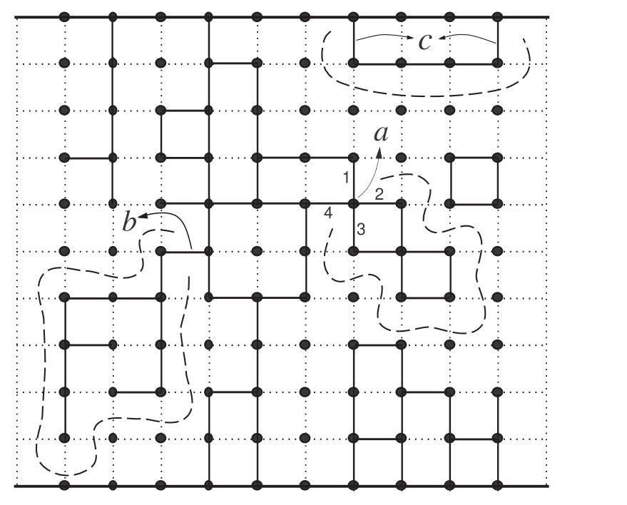
Below we give the definitions of all terminologies involved and illustrate them in a square lattice having $L$ sites horizontally and $L+1$ sites vertically (see Figure 1). Between neighboring sites we insert a bond that is taken to be open with an independent probability $p$, or closed with probability $1-p$. Obviously, here is defined the percolation model for bonds [20]. Open lateral boundary conditions are assumed, whereas all bonds locating at the top and the bottom are set open. A potential difference is applied between the top and the bottom. Two neighboring sites are connected to each other if the bond between them is open. The spanning cluster is the set of sites if there is a path of open bonds from each of them to the bottom and to the top. The spanning cluster consists of the current-carrying backbone and non-current-carrying dangling parts. There are three kinds of dangling parts of the spanning cluster: dangling ends, dangling arcs, and dangling loops. A dangling end is connected to the spanning cluster by only one open bond (e.g., $b$ in Figure 1); A dangling arc disconnects with the top (bottom) but is connected to the bottom (top) by at least two open bonds (e.g., $c$’s in Figure 1); A dangling loop is connected by at least two open bonds to only one site of the spanning cluster (e.g., $a$ in Figure 1). Here we name this site a dangling-loop-connecting site, which is called an articulation node in computer science. After all dangling parts are removed, the remainder of the spanning cluster is the backbone.

Our algorithm is based on Jordan’s curve theorem: Suppose there is a loop in a two-dimensional graph, then the area inside the loop disconnects with the area outside, and vise versa.

To make use of the theorem, we introduce the concept of plaquette that is an as small as possible area enclosed by a loop of bonds which can be either open or closed. For example, any one of the smallest square areas in Figure 1. We define that two nearest neighboring plaquettes are connected if the bond between them is closed. Note that the definition of connectedness for plaquettes is opposite to that for sites. Jordan’s curve theorem tells us that any dangling part must be enclosed by a loop of connected plaquettes if it is split from the spanning cluster. Hence, by use of the connectedness of plaquettes, we are able to identify dangling parts according to the following three corollaries of the theorem, which describe the local properties of the three kinds of dangling parts, respectively. We will directly use them to design our algorithm.

Corollary 1. An open bond connects a dangling end to the spanning cluster if and only if two plaquettes beside the bond are connected. For example, $b$ in Figure 1.

Corollary 2. If two non-neighboring plaquettes nearest neighboring the top (bottom) are connected, all sites that are connected to the top (bottom) by the bonds between the two plaquettes belong to dangling arcs. For example, $c$ in Figure 1.

Corollary 3. Let all dangling ends and arcs have been removed. Site $a$ is a dangling-loop-connecting site if and only if (i) $a$ connects at least four open bonds, referred to as bonds 1,2,3,4, and (ii) among its neighboring plaquettes, some between two of the four bonds (e.g., bonds 1 and 2) is connected by a path of plaquettes to some others between the other two bonds (i.e., bonds 3 and 4). For example, $a$ in Figure 1. $a$’s northern, eastern, southern, and western open bonds correspond to bonds 1, 2, 3, 4, respectively. $a$’s northeast plaquette which is between bonds 1 and 2 is connected by a path of plaquettes to $a$’s southwest plaquette which is between bonds 3 and 4. Note that here bonds 1 and 4 belong to the backbone, bonds 2 and 3 belong to a dangling loop.

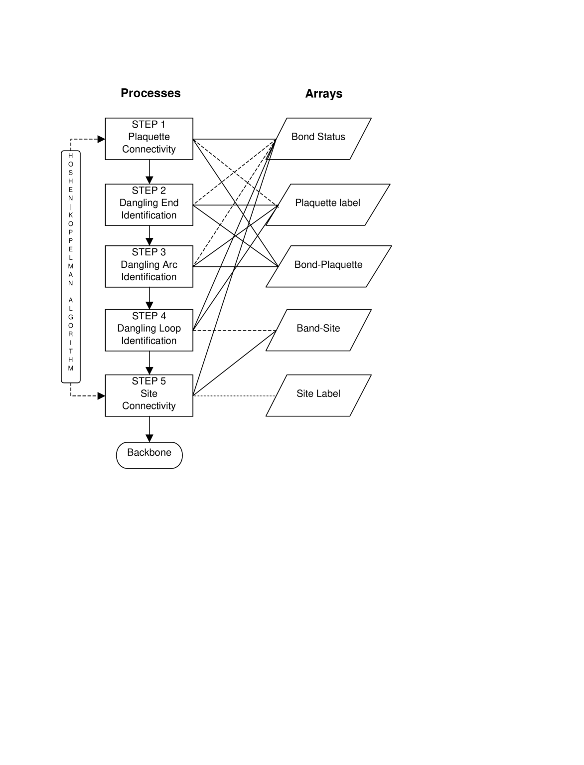
Now let us describe the procedure of our algorithm. In accordance with open lateral boundary conditions, the left (right) plaquettes of the leftmost (rightmost) column of vertical bonds are set to be the same, respectively, as shown in Figure 1. The algorithm is carried out as follows (see Figure 2).

Step 1. Compute the connectedness of plaquettes. If the leftmost plaquette is connected to the rightmost plaquette by a path of plaquettes, the spanning cluster does not exist [21].

Step 2 for identifying dangling ends. Sweep the bond graph to close any bond whose two-side plaquettes have the same label. This is the application of Corollary 1.

Step 3 for identifying dangling arcs. If two plaquettes neighboring the top (or the bottom) have the same label, then close all bonds between the two plaquettes. This is the application of Corollary 2.

Step 4 for identifying dangling loops. We look for dangling-loop-connecting sites ($a$) using Corollary 3. That is, $a$ connects four open bonds, referred to as bonds 1,2,3,4, and a plaquette between bond 1 and 2 has the same label as a plaquette between bond 3 and 4. Note that $a$’s themselves belong to the backbone. We use the following trick to split dangling loops: We create a new site $a^{\prime}$ and let bonds 2 and 3 be connected to $a^{\prime}$ instead of $a$. As a result, the subgraph connected to bonds 2 and 3 is disconnected to that connected to bonds 1 and 4.

Step 5. Compute the connectedness of sites including those newly created sites ($a^{\prime}$). The resultant spanning cluster is exactly the backbone.

In this paper, the connectedness of plaquettes or sites is calculated by using the modified Hoshen-Kopelman cluster-labeling algorithm [5, 15]. The data structure of this algorithm includes a bond status array that records the status of any bond [22], a site label array that records the label of any site (connected sites will have the same label), and a bond-site array that records two end sites of any bond. Our algorithm needs two extra arrays to record the information of plaquettes. One is a plaquette label array that records the label of any plaquette (connected plaquettes will have the same label), the other is a bond-plaquette array that records two side plaquettes of any bond. Given this data structure, we can compute both the connectedness of sites and the connectedness of plaquettes. The processes of the algorithm and the usage of the arrays are summarized in Figure 2. Only the bond status array is used in all steps. It is clear that if the memory is the bottle-neck of calculations, the bond-site array and the bond-plaquette array can occupy the same memory, so can the site label array and the plaquette array. The reasons are (i) they are not used simultaneously and (ii) they are used sequentially. The bond-plaquette array is used in Step 1-3 while the bond-site array is used in Step 4-5. The plaquette label array is used in Step 1-4 while the site label array is used in Step 5.

Figure 3 shows one of the simplest $d=2$ nonplanar graphs: a square lattice with both nearest neighboring (nn) bonds and next nearest neighboring (nnn) bonds. This type of nonplanar graphs is important because it is often used to mimic the effects of higher dimensionality [16]. Here a plaquette is a smallest triangular area. While a nn bond still has two side plaquettes, a nnn bond has four which are divided into two pairs by another nnn bond. If any pair of side plaquettes of a nnn bond have the same label, the nnn bond can be closed in Step 2. The number of bonds (plaquettes) in this case is twice (four times) as large as that in the corresponding planar square lattice with nn bonds only.

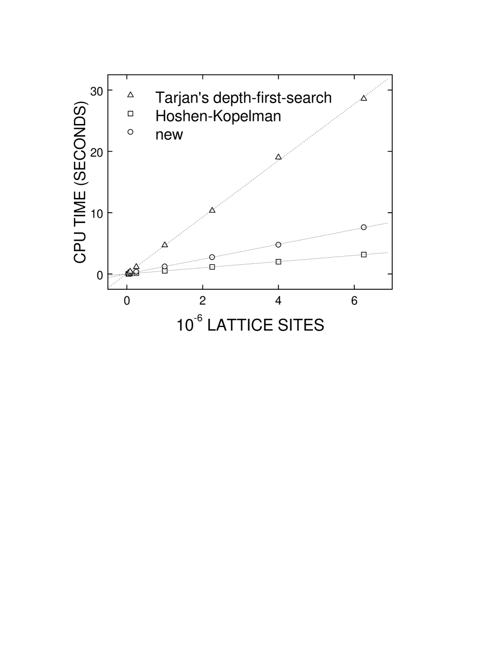
The efficiency of our algorithm is demonstrated in Figure 4 for square lattices with nn bonds only, where the central-processing-unit (CPU) time needed for the simulation is plotted versus the number of sites. We consider bond percolation at $p=p^{\rm(b)}_{\rm c}=0.5$ [4] and site percolation [20] at $p=p^{\rm(s)}_{\rm c}=0.592745(2)$ [23]. The results are obtained by averaging over 1000 configurations [22] for linear size $L=100,200,300,500,1000,1500,2000,2500$, respectively. Results for systems of larger size and more configurations will be reported soon. The calculations are carried out on a Pentium II/233 processor with Red Hat Linux release 4.2 operating system and GNU project F77 Compiler (v0.5.18). As shown in Figure 4, the dotted lines are our fits to the data for three algorithms. Their slopes are 0.51, 1.21, and 4.62 for the modified Hoshen-Kopelman algorithm, our new algorithm, and Tarjan’s depth-first-search algorithm, respectively. All the three algorithms run in time proportional to the system size. The total time needed to find the backbone is about twice as many as that to compute the connected cluster, since we use the modified Hoshen-Kopelman algorithm twice in the former and once in the latter. The present algorithm finds the current-carrying backbone almost four times as fast as Tarjan’s depth-first-search algorithm. Note that in our algorithm finding the backbone is not subject to finding the spanning cluster first. An advantage of the new algorithm is that it is easy to program and maintain because it involves only three local properties of dangling parts and uses the well-known modified Hoshen-Kopelman algorithm. The codes of the algorithm are available from us.

There are other algorithms for backbone identification [6, 7, 9, 11, 17]. A brief review of them was recently given in Ref. [13]. Here we make a comparison between ours and these known algorithm. The traditionally used algorithm by physicists is the burning algorithm [6, 7], which is at least for large $N$ much slower than Tarjan’s algorithm [13]. The matching algorithm with complexity slight larger than $N$ [$O(N^{1.07})$ for $d=2$] was used recently in literature [9]. For strictly planar graphs, the hull-generating algorithm is even faster [10, 11]. This algorithm has the same asymptotic complexity as Tarjan’s algorithm, but it is roughly twice as fast and uses about half of the memory, since it needs one data structure less and needs only one pass through all sites, instead of two passes in Tarjan’s algorithm [13]. For planar graphs, our algorithm is almost four times as fast as Tarjan’s algorithm and uses the memory of the same size as the modified Hoshen-Kopelman algorithm. For site percolation [20], a modified version of our algorithm uses the memory of even smaller size where the bond-site array and the bond-plaquette array are discarded [17]. Since the hull-generating algorithm, Tarjan’s, and ours have the same asymptotic complexity, their difference in speed is determined by the complexity of inner operations. Note that the identification of the backbone or the spanning cluster involves the global properties of sites. Our algorithm has an advantage such that it is able to identify dangling parts using their local properties complemented by the most efficient algorithm computing the connectedness of sites, which is currently the modified Hoshen-Kopelman algorithm. The modified Hoshen-Kopelman algorithm was originally used to identify the spanning cluster [5]. Because of its simplicity, the geometrical properties of the spanning cluster have been numerically studied on very large systems containing as much as $10^{11}$ sites [5]. Therefore, the inner operations of our algorithm are simpler than those of Tarjan’s and hull-generating. It should be made clear that the algorithms of Tarjan, matching, and burning can be used for arbitrary graphs; the hull-generating algorithm is valid for strictly planar graphs only; ours applies to general $d=2$ graphs with open literal boundary conditions, and thus has a wider range of application than the hull-generating algorithm.

The exact finding of the spanning cluster and the backbone enables us to calculate some scaling exponents for percolation. The order parameter of percolation is $P_{\infty}$, the ratio of the sites in the spanning cluster to all sites in the system. Correspondingly, we define $Q_{\infty}$, the ratio of the sites in the backbone to all sites in the system. These quantities scale with linear size $L$ as

$$P_{\infty}(L)\sim L^{-\beta/\nu},\hskip 7.11317ptQ_{\infty}(L)\sim L^{-q/\nu},\hskip 7.11317pt{\rm for}\,\,L\rightarrow\infty$$ (1)

where $\beta$, $q$, and $\nu$ are the critical exponents of $P_{\infty}$, $Q_{\infty}$, and the correlation length, respectively.

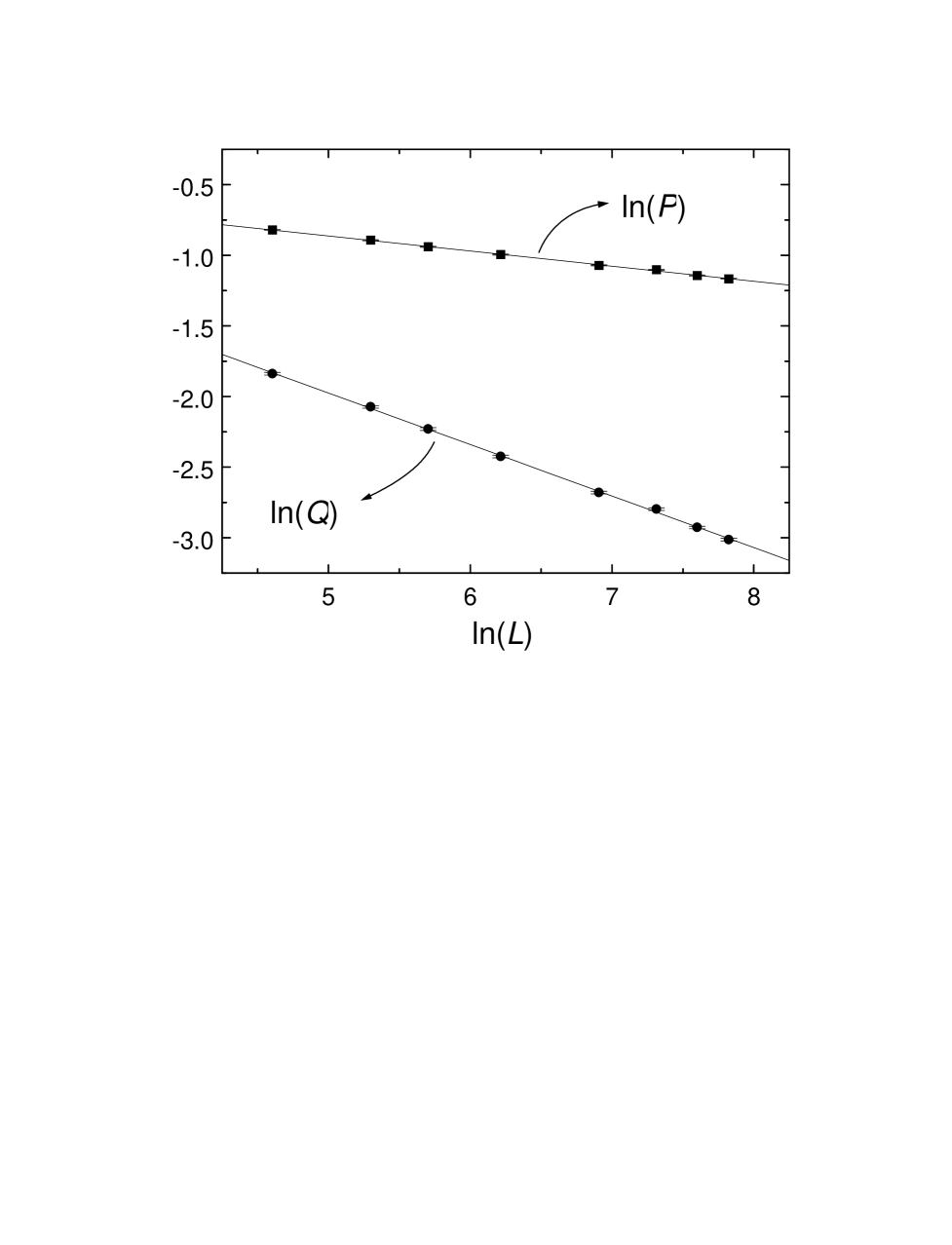
We calculate these scaling exponents in our Monte Carlo runs. Note that the following numerics are listed for demonstration because we have not calculated them on a world-record-breaking number of world-record-breaking scale lattices. The largest size considered here is $L=2500$ with 1000 configurations. Results for $L_{\rm max}=4096$ with 198470 configurations were reported in Ref. [13]. Calculations for systems of larger size and more configurations are in progress. The data are plotted in Figure 5 with very small standard errors of the mean. The lines shown in the log-log plot are the results of the weighted-least-squares fits, and yield the value $\beta/\nu=0.1068\pm 0.0013$ (close to the exact result $\beta/\nu=5/48$ [2, 5]), and $q/\nu=0.3647\pm 0.0039$. The calculated exponents satisfy the Chayes’ exponent inequalities [19]:

$$2\beta\leq q\leq t,$$ (2)

where $t$ is the exponent of conductivity (the best estimate for two-dimensional systems known to us is $t/\nu=0.9745\pm 0.0015$ [24]). The critical behavior of the backbone is consistently closer to that of the conductivity than that of the spanning cluster. Since $Q_{\infty}/P_{\infty}$ vanishes as $p\to p_{\rm c}$, the unknowns in the calculation of conductivity on the backbone is considerably less than those on the spanning cluster. As a result, the calculation of electronic conductivity on the backbone has considerably less statistical fluctuation and much reduced critical slowing down than on the spanning cluster [15].

Summarizing, we present a fast algorithm for identifying percolation backbones in general two-dimensional graphs with open boundary conditions. Complemented by the modified Hoshen-Kopelman algorithm, our algorithm identifies dangling parts using their local properties. For planar graphs, our algorithm is by far the fastest algorithm for backbone identification: it finds the backbone almost four times as fast as Tarjan’s depth-first-search algorithm, and uses the memory of the same size as the modified Hoshen-Kopelman algorithm.

We thank Paul Bastiaansen for providing us with the code of Tarjan’s depth-first-search algorithm implemented by J. Goodman (Ref. [15]) and M. E. J. Newman for pointing out the original hull-generating algorithm (Ref. [10]) and his recent work (Ref. [14]). We are grateful to our referees for their useful suggestions and pointing out recent important work done on the problem of percolation backbones (Ref. [6, 7, 9, 11, 13]). W.G.Y. was supported by the China Postdoctoral Science Foundation and the Shanghai Postdoctoral Science Foundation, and is supported by CUHK 4288/00P 2160148. R.T. was supported by the National Natural Science Foundation of China (No. 19774020), the foundation of Educational Ministry of China (No. 99024610), and Shanghai Research Center of Applied Physics.

FIG. 1.: An illustration of percolation on a square lattice of linear size $L=10$: site (filled circle), open bond (solid line), closed bond (dotted line), plaquette (smallest square area). $a$ is a dangling-loop-connecting site, $b$ is an open bond connecting a dangling end, and $c$ are open bonds belonging to a dangling arc. Dashed lines are some paths of connected plaquettes enclosing some dangling parts.

FIG. 2.: Flowchart of our algorithm. A line between an array (parallelogram) and a process (rectangle) indicates that the array is used in the process. If the line is dashed, the array changes in the process.

FIG. 3.: A square lattice of linear size $L=2$ with crossing bonds ($\overline{ac}$ and $\overline{bd}$). Filled circles $a,b,c,d$ denote sites. The smallest trianglular areas $1,2,3,4$ denote plaquettes. Bond $\overline{ac}$ has two pairs of side plaquettes [$(1,2)$ and $(3,4)$]. Bond $\overline{bd}$ has two pairs of side plaquettes [$(1,4)$ and $(2,3)$]. If any pair of side plaquettes of a crossing bond have the same label, the crossing bond can be closed.

FIG. 4.: CPU time of three algorithms for bond percolation at $p=p^{\rm(b)}_{\rm c}=0.5$. The dotted lines are our fits to the data. Their slopes are 0.51, 1.21, and 4.62 for the modified Hoshen-Kopelman algorithm, the new algorithm, and Tarjan’s depth-first-search algorithm, respectively.

FIG. 5.: Log-Log plot of $Q_{\infty}$ and $P_{\infty}$ for site percolation at $p=p^{\rm(s)}_{\rm c}=0.5927$. The dotted lines are the results of our weighted-least-squares fits against the functions $Q_{\infty}(L)=aL^{-q/\nu}$ and $P_{\infty}=bL^{-\beta/\nu}$, giving values of $q/\nu=0.3647\pm 0.0039$ and $\beta/\nu=0.1068\pm 0.0013$.

REFERENCES

- [1] Permanent electronic address: wgyin@yahoo.com.
- [2] D. Stauffer and A. Aharony, Introduction to Percolation Theory, 2nd edition (Taylor & Francis, Philadelphia, DA, 1994).
- [3] S. Kirkpatrick, Rev. Mod. Phys. 45, 574 (1973).
- [4] J. W. Essam, in: Phase Transitions and Critical Phenomena, Vol. 2, ed. C. Domb and M. S. Green (Academic, New York, 1972) pp. 218.
- [5] J. Hoshen and R. Kopelman, Phys. Rev. B 14, 3438 (1976); H. Nakanishi and H. E. Stanley, ibid. 22, 2466 (1980); A. Margolina, H. Nakanishi, D. Stauffer, and H. E. Stanley, J. Phy. A 17, 1683 (1984); D. C. Rapaport, J. Stat. Phys. 66, 679 (1992); H. Gould and J. Tobochnik, An Introduction to Computer Simulation Methods (Addison-Wesley, Reading, MA, 1988), Part 2, pp. 397-443; pp. 637-645.
- [6] M. D. Rintoul and H. Nakanishi, J. Phys. A 27, 5445 (1994); ibid. 25, L945 (1994).
- [7] H. J. Herrmann, D. C. Hong, H. E. Stanley, J. Phys. A 17, L261 (1984); H. J. Herrmann and H. E. Stanley, ibid. 21, L829 (1988); S. Roux and A. Hansen, ibid. 20, L1281 (1987); M. Porto, A. Bunde, S. Havlin, and H. E. Roman, Phys. Rev. E 56, 1667 (1997).
- [8] R. Tarjan, SIAM J. Comput. 1, 146 (1972); A. V. Aho, J. E. Hopcroft, and J. D. Ullman, The Design and Analysis of Computer Algorithms (Addison-Wesley, Reading, MA, 1974) pp. 176-187.
- [9] C. Moukarzel, Int. J. Mod. Phys. C 9, 887 (1998).
- [10] R. M. Ziff, P. T. Cummings, and G. Stell, J. Phys. A 17, 3009 (1984).
- [11] P. Grassberger, J. Phys. A 25, 5475 (1992).
- [12] C. J. Lobb and D. J. Frank, Phys. Rev. B 30, 4090 (1984); ibid. 37, 302 (1988).
- [13] P. Grassberger, Physica A 262, 251 (1999).
- [14] M. E. J. Newman and R. M. Ziff, Phys. Rev. Lett. 85, 4104 (2000).
- [15] R. G. Edwards, J. Goodman, and A. D. Sokal, Phys. Rev. Lett. 61, 1333 (1988); J. Ruge and K. Stuben, in Multigrid Methods, edited by S. F. McCormick (SIAM, Philadelphia, 1987).
- [16] P. Bastiaansen and H. Knops, J. Phys. A 30, 1791 (1997).
- [17] Wei-Guo Yin and Ruibao Tao, Physica B 279, 84 (2000).
- [18] Wei-Guo Yin and Ruibao Tao, Phys. Rev. B 62, 550 (2000).
- [19] J. T. Chayes and L. Chayes, Phys. Rev. Lett. 56, 1619 (1986); Comm. Math. Phys. 105, 133 (1986).
- [20] Percolation, of course, can be defined for sites. In this case, each site is taken to be occupied with probability or vacant with probability , and a bond is open if and only if both its end sites are occupied. But in the language of graph theory bond percolation is more general because the graphs created by site percolation are induced subgraphs of the lattice.
- [21] It is not true for percolation with periodic lateral boundary conditions.
- [22] Configurations are produced by randomly producing the bond status array: and . Open bonds appear with an independent probability .
- [23] R. M. Ziff and B. Sapoval, J. Phys. A 19, L1169 (1986).
- [24] J. M. Normand, H. J. Herrmann, and M. Hajjar, J. Stat. Phys. 52, 441 (1988).