Theory of spin wave excitations of metallic A-type antiferromagnetic manganites

Abstract

The spin dynamics of the metallic A-type antiferromagnetic manganites is studied. An effective nearest-neighbour Heisenberg spin wave dispersion is derived from the double exchange model taking into account the superexchange interaction between the core spins. The result of inelastic neutron scattering experiment on ${\rm Nd}_{0.45}{\rm Sr}_{0.55}{\rm Mn}{\rm O}_{3}$ is qualitatively reproduced. Comparing theory with experimental data two main parameters of the model: nearest-neighbour electron transfer amplitude and superexchange coupling between the core spins are estimated.

Interest in the doped manganese oxides with perovskite structure ${\rm R}_{1-x}{\rm B}_{x}{\rm MnO}_{3}$ (where ${\rm R}$ is trivalent rare–earth and ${\rm B}$ is divalent alkaline ion, respectively) has revived since the discovery of colossal magnetoresistance (CMR) in those compounds.[2]

Extensive experimental study of the doped manganites has revealed unusual microscopical structures of spin–, charge–, and orbital–ordered states.[3] At different doping concentration a full range of magnetically ordered states such as antiferromagnetic (AFM) insulator, ferromagnetic (FM) metal and charge ordered (CO) insulator have been observed. The importance of the charge, spin as well as orbital[4] and lattice [5] degrees of freedom and of interplay between them has now been well established.

In the ideal undistorted perovskite structure ${\rm Mn}$ ions are surrounded by six oxygen ions, and form a simple cubic lattice with the trivalent rare-earth ion sitting in the center of the cube. The six oxygen ions, ${\rm O}^{2-}$, forming the octahedra give rise to the crystal field potential that removes the degeneracy of $d$ orbital of manganese. As a result $d$ level is splitted into $t_{2g}$ triplet ($d_{xy}$, $d_{xz}$, and $d_{yz}$) and $e_{g}$ doublet ($d_{3z^{2}-r^{2}}$, and $d_{x^{2}-y^{2}}$). The orbitals $d_{3z^{2}-r^{2}}$, and $d_{x^{2}-y^{2}}$ are degenerate and since they point toward the ${\rm O}^{2-}$ ions they have higher energy then the $t_{2g}$ orbitals. The $t_{2g}$ electrons are strongly coupled by intra-atomic Hund’s coupling in the high spin state $S=3/2$, and remain localized even in doped compounds. The $e_{g}$ electrons are subject to strong Hund’s coupling with the core spin, they are localized in the undoped compounds (one $e_{g}$ electron per manganese ion) due to the strong intra-atomic Coulomb repulsion.

The reference undoped compound ${\rm La}{\rm Mn}{\rm O}_{3}$ is a Mott insulator with a spin $S=2$, and orbital degrees of freedom. Spins are ordered ferromagnetically in $(x,y)$ plane and antiferromagnetically in $z$ direction (so-called A-type AFM state).[6, 7] The orbitals are also ordered: in-plane directional orbitals $d_{3x^{2}-r^{2}}$ and $d_{3y^{2}-r^{2}}$ alternate in $(x,y)$ plane and are stacked in $z$ direction. This leads to the distortion of local surrounding of the Jahn-Teller (JT) active ${\rm Mn}$ ion, rezulting in elongation of ${\rm Mn}{\rm O}_{6}$ octahedra along $x$ ($y$) direction which has been observed experimentally.[8]

Upon doping of the parent compounds the $e_{g}$-electrons become mobile using oxygen’s $p$-orbitals as a bridge between ${\rm Mn}$ ions and the strong on-site Hund’s coupling drives core spins to align parallel forming the metallic FM ground state. The double exchange (DE) interaction[9] that mediates the ferromagnetic coupling between the core spins is the key ingredient in a appropriate interpretation of the phase diagram at the doping range $0.2<x<0.5$ where FM metallic behavior is observed.

Close to the half-doping ($x\sim 0.5$) the phase diagram becomes more subtle. The narrow band manganites (low $T_{\rm c}$ compounds) exhibit a charge ordered state close to the commensurate filling. This CO state is characterized by an alternating ${\rm Mn}^{3+}$ and ${\rm Mn}^{4}$ ions arrangement in the $(x,y)$ plane with charge stacking in $z$-direction. In addition, these systems show $d_{3x^{2}-r^{2}}$/$d_{3y^{2}-r^{2}}$ orbital ordering. In CO state these systems exhibit an insulating behavior with a very peculiar form of AFM spin ordering at low temperature. The observed magnetic structure is a CE-type and consists of quasi one-dimensional ferromagnetic zig-zag chains coupled antiferromagnetically.[6] A direct evidence of the CE charge/spin ordered state in half-doped manganites has been provided by the electron diffraction for ${\rm La}_{0.5}{\rm Ca}_{0.5}{\rm MnO}_{3}$.[10] Similar observations have also been reported for ${\rm Pr}_{0.5}{\rm Ca}_{0.5}{\rm MnO}_{3}$.[11, 12] All these compounds show paramagnetic insulating states at high temperature with predominant FM fluctuations.[11] Upon lowering the temperature the charge correlations together with orbital correlation develops. The FM fluctuations are first suppressed at charge/orbital ordering temperature $T_{\rm o}$ and completely disappear at the AFM ordering temperature $T_{\rm N}$.[11] And finally, at $T<T_{\rm N}$ a CE charge/spin/orbital ordered state is established.

It is clear that all the degrees of freedom involved in the formation of ground state are strongly coupled at commensurate doping. Then the symmetry of the ground state is dictated by the competition between the hopping driven ferromagnetic exchange, antiferromagnetic superexchange (SE), electrostatic and lattice elastic energies. This competition has been studied in detail to interpret the rather complicated CE spin/charge/orbital ordered state observed in half-doped manganites.[7, 13, 14]

In the moderately narrow band system ${\rm Nd}_{0.5}{\rm Sr}_{0.5}{\rm MnO}_{3}$[15] and ${\rm Pr}_{0.5}{\rm Sr}_{0.5}{\rm MnO}_{3}$[16] CO state has been observed in very narrow band region of ${\rm Sr}$ concentration around $x\sim 0.5$.

However, in a recent experimental study of ${\rm Pr}_{0.5}{\rm Sr}_{0.5}{\rm MnO}_{3}$ and ${\rm Nd}_{0.45}{\rm Sr}_{0.55}{\rm MnO}_{3}$ it was found[17] that instead of the well known CE charge/spin/orbital ordered state both systems show A-type AFM order in the ground state with uniform $d_{x^{2}-y^{2}}$ orbital order and no clear sign of the charge ordering. The A-type AFM order has been also confirmed by the large anisotropy in resistivity and spin wave measurements.[18]

This finding is consistent with recently obtained mean–field phase digram of two–orbital double–exchange model.[14] It was shown that A-type AFM state and charge ordering do not coexist. The A-type spin ordering is unstable against the formation CE-type magnetic structure when charge ordering is introduced in the system. In the CO state the carrier kinetic energy and hence double exchange energy are suppressed, and the CE spin/charge ordered state is more favorable due to the additional gain in energy by modulating the FM bonds in basal plane and generating a ”dimerization”–like gap at the Fermi surface due to a staggered factor in electron hopping amplitude.

In the present paper we propose the spin wave theory of such an A-type metallic state. We show that the spin wave excitation spectrum derived in the leading order of $1/S$ expansion of the double exchange model in A-type metallic state reproduces the spin wave dispersion relation observed recently in the inelastic neutron scattering experiment on ${\rm Nd}_{0.45}{\rm Sr}_{0.55}{\rm MnO}_{3}$.[18] Fitting theory to the experimental data gives an estimate of effective transfer integral, as well as the AFM superexchange coupling between the $t_{2g}$ core spins.

In the A-type AFM state electrons are confined in the basal plane due to the large Hund’s coupling. Since the transfer integral between $d_{x^{2}-y^{2}}$ orbitals is largest in the $(x,y)$ plane, the low energy eigen state of two orbital tight–binding Hamiltonian has mainly $d_{x^{2}-y^{2}}$ character. Hence there exists an anisotropy in orbital occupation, even in the absence of JT coupling. Including JT effect will lead to a farther increase of the anisotropy and the splitting between $d_{x^{2}-y^{2}}$ and $d_{3z^{2}-r^{2}}$ levels. Therefore, in our model we retain only the relevant $d_{x^{2}-y^{2}}$ orbital, and also assume that all the other degrees of freedom are integrated out to give effective model parameters. We start with the Hamiltonian:

$$H = -t\sum_{\langle ij\rangle\parallel,\sigma}\left[d_{i\sigma}^{\dagger}d_{j\sigma}+H.c.\right]-\mu\sum_{i}n_{i}$$ (1)

$$- J_{\rm H}\sum_{i}{\bf S}_{i}{\bf\sigma}_{i}+J\sum_{\langle ij\rangle}{\bf S}_{i}{\bf S}_{j}.$$ (2)

The first term in Eq.(2) describes an electron hopping between the the nearest neighbor (NN) Mn-ions in $(x,y)$ plane, with $t$ being the transfer amplitude between $d_{x^{2}-y^{2}}$ orbitals. The second term describes the Hund’s coupling between the spins of localized $t_{2g}$- electrons ${\bf S}_{i}$ and the itinerant $e_{g}$ electrons with spin ${\bf\sigma}_{i}$. The superexchange interaction of localized spins between the NN sites is given by $J$, $n_{i}$ is the particle number operator and $\mu$ is the chemical potential.

Next step is to introduce two sublattices $A$ and $B$ with spin up and down for the alternating in $z$-direction plains in A-type AFM state. Then we can expand the core spin operators by the Holstein-Primakoff transformation as follows:

$$S_{i}^{+}=\left\{\begin{array}[]{ll}\sqrt{2S}\alpha_{i}&\textrm{if $i\in A$}\\ \sqrt{2S}\beta_{i}^{\dagger}&\textrm{if $i\in B$}\\ \end{array}\right.~{},\;\;S_{i}^{-}=\left\{\begin{array}[]{ll}\sqrt{2S}\alpha_{i}^{\dagger}&\textrm{if $i\in A$}\\ \sqrt{2S}\beta_{i}&\textrm{if $i\in B$}\\ \end{array}\right.~{},$$

$$S_{i}^{z}=\left\{\begin{array}[]{ll}S-\alpha_{i}^{\dagger}\alpha_{i}&\textrm{if $i\in A$}\\ -S+\beta_{i}^{\dagger}\beta{i}&\textrm{if $i\in B$}\\ \end{array}\right.~{}.$$ (5)

By substituting expressions (5) into the Hamiltonian (2) and keeping the terms contributing to leading order in $1/S$ expansion we obtain the following Hamiltonian in the momentum space $H=H_{\text{el}}+H_{\text{sw}}+H_{\text{int}},$ where $H_{\text{el}}$ and $H_{\text{sw}}$ describe the charge and spin degrees of freedom, respectively and interaction among them are given by $H_{\text{int}}$:

$$H_{\text{el}} = \sum_{{\bf k}\sigma}\epsilon_{{\bf k}\sigma}\left[a_{{\bf k}\sigma}^{\dagger}a_{{\bf k}\sigma}+b_{{\bf k}\bar{\sigma}}^{\dagger}b_{{\bf k}\bar{\sigma}}\right],$$ (6)

$$H_{\text{sw}} = \sum_{\bf q}\left[\omega_{0,{\bf q}}\left(\alpha_{\bf q}^{\dagger}\alpha_{\bf q}+\beta_{\bf q}^{\dagger}\beta_{\bf q}\right)+\left(\Omega_{{\bf q}}\alpha_{\bf q}^{\dagger}\beta_{-{\bf q}}^{\dagger}+\text{H.c.}\right)\right],$$ (7)

$$H_{\text{int}} = -\frac{J_{\rm H}\sqrt{S}}{\sqrt{2N}}\sum_{{\bf k,\bf q}}\left[a_{{\bf k}\uparrow}^{\dagger}a_{{\bf k}+{\bf q}\downarrow}\alpha_{\bf q}^{\dagger}+b_{{\bf k}\downarrow}^{\dagger}b_{{\bf k}+{\bf q}\uparrow}\beta_{\bf q}^{\dagger}+\text{H.c.}\right]$$ (8)

where $a_{{\bf k}\sigma}$ and $b_{{\bf k}\sigma}$ stands for the electrons on $A$ and $B$ sublattice, respectively, $\epsilon_{{\bf k},\uparrow(\downarrow)}=-4t\gamma_{\parallel{\bf k}}\mp J_{\text{H}}S/2-\mu$ is the electron dispersion in $(x,y)$ plane including Zeeman splitting, $\gamma_{\parallel{\bf k}}=1/2(\cos k_{x}+\cos k_{y})$, $\omega_{0,{\bf q}}=J_{\text{H}}m+2JS-4JS(1-\gamma_{\parallel{\bf q}})$, $\Omega_{\bf q}=JS(1+e^{-2iq_{z}})$, and $m=1/2(n_{a,\uparrow}-n_{a,\downarrow})=-1/2(n_{b,\uparrow}-n_{b,\downarrow})$ is the magnetization of electron subsystem. In the state with fully polarized FM planes considered here $m=n/2$ with $n$ being the electron density.

The spin wave part of the Hamiltonian $H_{\text{sw}}$ (6) is diagonalized by the standard Bogoliubov transformation

$$\alpha_{\bf q}=e^{-iq_{z}}[u_{{\bf q}}\hat{\alpha}_{\bf q}+v_{{\bf q}}\hat{\beta}^{\dagger}_{\bf-q}],\;\beta_{-{\bf q}}^{\dagger}=-v_{{\bf q}}\hat{\alpha}_{\bf q}+u_{{\bf q}}\hat{\beta}^{\dagger}_{\bf-q}$$ (9)

bringing it into the form

$$H_{\text{sw}}=\sum_{\bf q}\omega_{{\bf q}}\left[\hat{\alpha}^{\dagger}_{\bf q}\hat{\alpha}_{\bf q}+\hat{\beta}^{\dagger}_{\bf q}\hat{\beta}_{\bf q}\right].$$ (10)

The eigen–frequency $\omega_{{\bf q}}$ and the coherence factors are given by

$$u_{{\bf q}} = \frac{1}{\sqrt{2}}\left[1+\frac{\omega_{0,{\bf q}}}{\omega_{{\bf q}}}\right]^{1/2},\;v_{{\bf q}}=\frac{1}{\sqrt{2}}\left[1-\frac{\omega_{0,{\bf q}}}{\omega_{{\bf q}}}\right]^{1/2},$$ (11)

$$\omega_{{\bf q}} = \sqrt{\omega_{0,{\bf q}}^{2}-|\Omega_{{\bf q}}|^{2}}.$$ (12)

Next we introduce the Fourier transformed retarded matrix Green function (GF) for magnons ${\mathsf{D}}_{{\bf q},\omega}=\ll{\mathsf{A}}_{{\bf q}}|{\mathsf{A}}_{{\bf q}}^{\dagger}\gg_{\omega}$ where, ${\mathsf{A}}_{{\bf q}}$ is the two–component operator and $A_{{\bf q}}^{\dagger}=(\alpha_{{\bf q}}^{\dagger},\;\beta_{-{\bf q}})$. The components of $\cal{D}_{{\bf q},\omega}$ are however related among each-other by symmetry relations and hereafter we consider the diagonal (normal) $(\cal D)$ and non-diagonal (anomalous) $(\hat{\cal D})$ components, expressing them in terms of the self-energy operators via the Dyson-Beliaev equation

$${\cal D}_{{\bf q},\omega} = \frac{\omega+\omega_{\bf q}+\Sigma_{{\bf q},-\omega}}{{D}_{{\bf q},{\omega}}}~{},\;\;\;\hat{\cal D}_{{\bf q},\omega}=\frac{-\hat{\Sigma}_{{\bf q},\omega}}{{D}_{{\bf q},{\omega}}}~{},$$ (13)

where the following notations has been introduced:

$${D}_{{\bf q},{\omega}} = [\omega-{\cal A}_{{\bf q},\omega}]^{2}-[\omega_{\bf q}+S_{{\bf q},\omega}^{-}][\omega_{\bf q}+S_{{\bf q},\omega}^{+}]~{},$$ (14)

$${\cal A}_{{\bf q},\omega} = \frac{\Sigma_{{\bf q},\omega}-\Sigma_{{\bf q},-\omega}}{2},\;{\cal S}_{{\bf q},\omega}^{-}=\frac{\Sigma_{{\bf q},\omega}+\Sigma_{{\bf q},-\omega}-2\hat{\Sigma}_{{\bf q},\omega}}{2},$$ (15)

$${\cal S}_{{\bf q},\omega}^{+} = \frac{\Sigma_{{\bf q},\omega}+\Sigma_{{\bf q},-\omega}+2\hat{\Sigma}_{{\bf q},\omega}}{2}~{}.$$ (16)

Here $\Sigma_{{\bf q},\omega}$ and $\hat{\Sigma}_{{\bf q},\omega}$ are normal and anomalous components of magnons self-energy due to the coupling with electrons, ${\cal A}_{{\bf q},\omega}$ is an antisymmetric function in $\omega$, while ${\cal S}_{{\bf q},\omega}$ and $\hat{\Sigma}_{{\bf q},\omega}$ are symmetric functions of $\omega$.

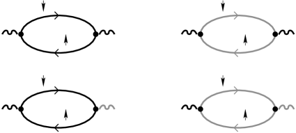
FIG. 1.: Graphical representation of the normal and anomalous components of the spin wave self-energy. The black and gray straight (wavy) lines stand for the electron (spin wave) propagators on $A$ and $B$ sublattices, respectively.

In the leading order of $1/S$ expansion, the self-energy operators ($\Sigma$ and $\hat{\Sigma}$) are given by the particle-hole bubble diagrams shown in Fig. 2. The black and gray lines stand for the electron propagators on $A$ and $B$ sublattices, respectively. The upper (lower) graphs corresponds to the normal (anomalous) component of the magnons self-energy. The anomalous part of the self-energy couples degenerate $\alpha$ and $\beta$ magnons denoted by black and gray wavy lines, respectively. The dot represents the magnon-fermion vertex, analytical form of which is easily obtained by reexpressing the interaction term of the Hamiltonian (6) in terms of transformed magnon operators. The above introduced dynamical quantities (14) have the following analytical expression:

$${\cal A}_{{\bf q},\omega} = \frac{J_{\text{H}}^{2}S}{2N}\sum_{{\bf k}}\frac{[n_{{\bf k}\uparrow}-n_{{\bf k+q}\downarrow}]\omega}{\omega^{2}-[\epsilon_{{\bf k+q}\downarrow}-\epsilon_{{\bf k}\uparrow}]^{2}}~{},$$ (17)

$${\cal S}_{{\bf q},\omega}^{\pm} = \frac{J_{\text{H}}^{2}S[u_{\bf q}\pm v_{\bf q}]^{2}}{2N}\sum_{{\bf k}}\frac{[n_{{\bf k}\uparrow}-n_{{\bf k+q}\downarrow}][\epsilon_{{\bf k+q}\downarrow}-\epsilon_{{\bf k}\uparrow}]}{\omega^{2}-[\epsilon_{{\bf k+q}\downarrow}-\epsilon_{{\bf k}\uparrow}]^{2}}~{},$$ (18)

where $n_{{\bf k}\sigma}=[e^{\epsilon_{{\bf k}\sigma}}+1]^{-1}$ is the Fermi distribution function.

The renormalized spin wave spectrum, arising from the second order self-energy corrections, are given by the poles of the magnons Green’s function (13), or equivalently by the zeros of ${D}_{{\bf q},{\omega}}$ (14). Assuming the large Hund’s coupling $J_{\text{H}}\gg t$, and expanding the self-energies up to leading order in $t/J_{H}$ the spin wave spectrum can be written as:

$${\tilde{\omega}}_{{\bf q}}=2S\sqrt{[J+2J_{\text{F}}(1-\gamma_{\parallel{\bf q}})]^{2}-J^{2}\gamma_{\perp{\bf q}}^{2}}~{},$$ (19)

where $\gamma_{\perp{\bf k}}=\cos k_{z}$ and the effective ferromagnetic exchange energy is given by

$$J_{\text{F}}=J_{\text{DE}}-J,\;\;\text{with}\;\;J_{\text{DE}}=t\langle a_{i\uparrow}^{\dagger}a_{j\uparrow}\rangle/(2S^{2})$$ (20)

being the double-exchange energy given by kinetic energy of electrons.

FIG. 2.: The spin wave dispersion of ${\rm Pr}_{0.5}{\rm Sr}_{0.5}{\rm Mn}{\rm O}_{3}$ from Ref.17 (the full circles and squares stand for ${\bf q}\parallel(1,0,0)$ and ${\bf q}\parallel(0,0,1)$, respectively). The solid curves represents fitting by Eq.19 including the anisotropy gap.

The obtained spin wave spectrum (19) corresponds to that of nearest-neighbor Heisenberg model with intraplane ferromagnetic exchange integral $J_{\text{F}}$ and antiferromagnetic interplane coupling $J$. The correspondence between spin dynamics in the FM phase of DE model and in effective NN Heisenberg model exist at quasi-classical level (i.e. leading order in $1/S$ expansion) and has been studied in Refs.[19].

The long wave-length behavior of the spin-wave dispersion is given by

$${\tilde{\omega}}_{{\bf q}}\propto\left\{\begin{array}[]{ll}C_{\parallel}q&\textrm{for ${\bf q}\parallel(1,0,0)$}\\ C_{\perp}q&\textrm{for ${\bf q}\parallel(0,0,1)$}\\ \end{array}\right.$$ (23)

where $C_{\parallel}=2S\sqrt{JJ_{\text{F}}}$ and $C_{\perp}=2SJ$ are intra– and inter–plane spin wave stiffness, respectively. Here we note, that long wave-length behavior of spin wave spectrum within the FM planes reduces to sound-like dispersion unlike the $q^{2}$ behavior inherent for isotropic ferromagnets.

Fig. 2 shows a fit of inelastic neutron scattering experiment for ${\rm Nd}_{0.45}{\rm Sr}_{0.55}{\rm Mn}{\rm O}_{3}$ from Ref.[18] using the obtained spin wave spectrum (19) including the phenomenological anisotropy gap ${\Delta}$. The full circles and squares stand for the experimental data in $(1,0,0)$ and $(0,0,1)$ direction respectively. As has already been pointed out in Ref.[18], the best fit is obtained for a intralayer FM exchange $4J_{\text{F}}S\simeq 32\text{meV}$, interlayer AFM exchange $2JS\simeq 10\text{meV}$, and $\Delta\simeq 0.26\text{meV}$. At $x=0.55$ NN correlation function $\langle a_{i\uparrow}^{\dagger}a_{j\uparrow}\rangle=0.2$ and from Eq.20 one obtains following estimates for $d_{x^{2}-y^{2}}$ transfer integral $t\simeq 0.195\text{eV}$ and AFM superexchange coupling $J\simeq 3.3\text{meV}$.

To summarize, the spin wave dispersion in A-type AFM state of the double exchange model is derived tacking into account the superexchange interaction between the core spins. The result of inelastic neutron scattering experiment on ${\rm Nd}_{0.45}{\rm Sr}_{0.55}{\rm Mn}{\rm O}_{3}$ is qualitatively reproduced. Comparison of theory with experimental data gives the estimates of two main parameters of the model: nearest-neighbor electron transfer amplitude $t$ and superexchange coupling between the core spins $J$. While the present estimate of AFM superexchange strength $J\simeq 3.3\text{meV}$ coincides with that widely used in the literature, [20] it is factor 4 times larger then SE integral estimated form the Neel temperature of the end compound ${\rm CaMnO}_{3}$ leading to $J\simeq 0.8\text{meV}$.[21] In ${\rm Sr}$ doped compounds the both $e_{g}$ and $t_{2g}$ ${\rm Mn}-{\rm O}$ transfer amplitudes ($t_{e}$ and $t_{g}$) are higher than that in ${\rm Ca}$ doped compounds due to the different ionic radii of these element leading to different ${\rm Mn}-{\rm O}$ distance and ${\rm Mn}-{\rm O}-{\rm Mn}$ bond angle. The AFM SE exchange is given by the forth power of the transfer amplitude $t_{e}^{4}$ ($t_{g}^{4}$) and hence a small increase of the latter might give a larger value of SE strength in Sr-doped compounds. This increase of magnetic frustration due to the increase of AFM SE strength going from ${\rm Sr}$ to ${\rm Ca}$ doped compounds has been also observed experimentally [22].

The authors acknowledge the kind hospitality at the Max-Plank Institute f$\ddot{\rm u}$r Physik komplexer Systeme, where the the present work has been carried out. Financial support by the INTAS Program, Grants No 97-0963 and No 97-11066, are also acknowledged. One of the authors (G.J.) is partly supported by the programme SCOPES of the Swiss National Science Foundation and the Federal Department of Foreign Affairs. G.J. would like to thank Nic Shannon and Victor Yu. Yushankhai for useful discussions.

REFERENCES

- [1] Permanent Address: Institute of Physics, Georgian Academy of Sciences, Tbilisi, Georgia.
- [2] R. von Helmolt, J. Wecker, B. Holzapfel, L. Schultz, and K. Samwer, Phys. Rev. Lett. 71, 2331 (1993); S. Jin, T. H. Tiefel, M. McCormack, R. A. Fastnacht, R Ramesh, and L. H. Chen, Science 264, 413 (1994).
- [3] For a review, see, for example, Colossal Magnetoresistive Oxides, edited by Y.Tokura (Gordon & Breach, New York, (2000), and references therein.
- [4] Y. Tokura, and N. Nagaosa, Science 288, 462 (2000).
- [5] A. J. Millis, P. B. Littlewood, and B. I. Shraiman, Phys. Rev. Lett. 74, 5144 (1995).
- [6] E. O. Wollan, W. C. Koehler, Phys. Rev. B. 100, 545, (1955).
- [7] J. B. Goodenough, Phys Rev. 100, 564 (1955).
- [8] J. Rodríguez-Carvajal, M. Hennion, F. Moussa, A. H. Moudden, L. Pinsard, and A. Revcolevschi, Phys. Rev. B 57, R3189 (1998); Y. Murakami, J. P. Hill, D. Gibbs, M. Blume, I. Koyama, M. Tanaka, H. Kawata, T. Arima, Y. Tokura, K. Hirota, and Y. Endoh, Phys. Rev. Lett. 81, 582 (1998).
- [9] C. Zener, Phys. Rev. 82, 403 (1951); P. W. Anderson, H. Hasegawa, Phys. Rev. 100, 675 (1955); P. G. de Gennes, Phys. Rev. 118, 141 (1960).
- [10] C.H. Chen and S.-W. Cheong, Phys. Rev. Lett. 76, 4042, (1996).
- [11] R. Kajimoto, T. Kakeshita, Y. Oohara, H. Yoshizawa, Y. Tomioka and Y.Tokura, Physica B 241-243, 436 (1998).
- [12] M. v. Zimmermann, J. P. Hill, Doon Gibbs, M. Blume, D. Casa, B. Keimer, Y. Murakami, Y. Tomioka, and Y. Tokura, Phys. Rev. Lett. 83, 4782 (1999).
- [13] I.Soloviev and K. Terakura, Phys. Rev. Lett. 83, 2825, (1999); J. van der Brink, G.Khaliulin and D.I.Khomskii, ibid. 83, 5118, (1999); S. Yunoki, T. Hotta and E. Dagotto, ibid 84, 3714 (2000).
- [14] G. Jackeli, N. B. Perkins, and N. M. Plakida, Phys. Rev. B 62, 372 (2000).
- [15] H. Kuwahara , Y. Tomioka, A. Asamitsu, Y. Morimoto, and Y.Tokura, Science 270, 961, (1995).
- [16] K. Knizek, Z.Jirak, E. Pollert, F. Zounova, S. Vratislav, J. Solid State Chem. 100, 292 (1992).
- [17] H. Kawano, R. Kajimoto, H. Yoshizawa, Y. Tomioka, Y. Kuwahara, and Y. Tokura, Phys. Rev. Lett. 78, 4253, (1997).
- [18] H. Yoshizawa, H. Kawano, J. A. Fernandez-Baca, H. Kuwahara, Y. Tokura, Phys. Rev. B bf 58, R571 (1998).
- [19] N. Kubo and N. Ohata, J. Phys. Soc. Jpn. 33, 21 (1972); N. Furukawa, J. Phys. Soc. Jpn. 63, 3214 (1994); N. B. Perkins and N. M. Plakida, Theor. Math. Phys. 120,1182 (1999); The next order-corrections in the expansion to the spin wave dynamics of DE model has been recently discussed by D. Golosov, Phys. Rev. Lett. 84, 3974 (2000); N. Shannon and A. V. Chubukov cond-mat/0011390 (unpublished).
- [20] S. K. Mishra, R. Pandit, and S. Satpathy, J. Phys.: Condens. Matter 11, 8561 (1999). For a recent review see: A. M. Oles, M. Cuoco, N. B. Perkins, AIP Conf. Proc. 527, 226 (New York 2000); E. Dagotto, T. Hotta, A. Moreo, cond-mat/0012179 (to be published in Phys. Rep.).
- [21] A. J. Millis, Phys. Rev. B 55, 6405 (1997).
- [22] J. L. García-Mnoz, J. Fomtcuberta, B. Martínez, A. Seffar, S. Piol, and X. Obradors, Phys. Rev. B 55, R668 (1997).