The $\pm J$ Spin Glass: Effects of Ground State Degeneracy

Abstract

We perform Monte Carlo simulations of the Ising spin glass at low temperature in three dimensions with a $\pm J$ distribution of couplings. Our results display crossover scaling between $T=0$ behavior, where the order parameter distribution $P(q)$ becomes trivial for $L\to\infty$, and finite-$T$ behavior, where the non-trivial part of $P(q)$ has a much weaker dependence on $L$, and is possibly size independent.

]

I Introduction

Several papers[1, 2, 3, 4] have recently studied the Ising spin glass in three dimensions with a Gaussian distribution of bonds at low and zero temperature. From data obtained on small sizes these papers deduce that the order parameter distribution function, $P(q)$, is non-trivial at finite-$T$, i.e. in addition to two peaks, symmetric about $q=0$, there is also a continuous part between the peaks whose weight does not decrease with size[5]. This indicates the existence of a nontrivial energy landscape, i.e. of macroscopic excitations, involving a finite fraction of the system, that cost a finite energy in the thermodynamic limit. This aspect of the results is consistent with the replica symmetry breaking picture of Parisi[6]. By contrast, the droplet theory[7, 8] predicts that the weight in the continuous part of the distribution should vanish like $L^{-\theta}$ as the (linear) size of the system $L$ increases, where $\theta$ is a positive exponent. In both theories, because the ground state is unique (apart from inverting all the spins), it follows that the weight in the “tail” of the distribution tends to zero (proportional to $T$) as $T\to 0$ and the positions of the peaks tend to $\pm 1$. The purpose of this paper is to see how these results are modified for a spin glass with a bimodal distribution (also called the $\pm J$ distribution), where the interactions have values $\pm 1$, where there is a large ground state degeneracy and a finite ground state entropy per spin.

One might possibly imagine that, since the system with the $\pm J$ distribution has a finite ground state entropy, its behavior at zero temperature would be similar to that of a model with continuous distribution at finite-$T$. If this were true then, according to the numerical results,[1, 2, 3, 4] $P(q)$ would be non-trivial at $T=0$ whereas according to the droplet theory $P(q)$ would be trivial.

However, this notion has been contested by Krzakala and Martin[9] (referred to henceforth as KM) who argue that entropy effects cause one “valley” in the $T=0$ energy landscape of the $\pm J$ model to dominate and consequently the weight in the tail vanishes like $L^{-\lambda}$, where $\lambda$ is a positive exponent (discussed below), even if the energy landscape is non-trivial. At finite-$T$, KM argue that the weight is finite for large $L$, so, by implication, there must be a crossover at some scale $L_{c}(T)$ from the $L^{-\lambda}$ behavior for $L<L_{c}(T)$ to a value independent of $L$ at larger sizes. One can also generalize the KM argument to the droplet model, in which case there is still a crossover, between $L^{-(\lambda+\theta)}$ behavior at smaller $L$ and $L^{-\theta}$ behavior at larger $L$. Overall, in the KM scenario, the only difference between the continuous and the $\pm J$ distributions for $L\gg L_{c}(T)$ is that the position of the peaks in $P(q)$ are different for $T\to 0$. Denoting the peak positions by $\pm q_{0}$, then one has $q_{0}<1$ for the $\pm J$ distribution whereas $q_{0}$ = 1 for a continuous distribution.

Here we display, we believe for the first time, the crossover between $T=0$ and finite-$T$ behaviors. Further motivation for our work is to clarify conflicting results for ground state properties. Berg et al.[10] used a multicanonical Monte Carlo technique to determine $P(q)$ at $T=0$ finding results consistent with trivial behavior with $\lambda=0.72\pm 0.12$ (but also not ruling out the possibility of nontrivial behavior). Hartmann[11] used a genetic optimization algorithm finding initially a nontrivial $P(q)$, but the results were biased[12] because the degenerate ground states were not sampled with equal probability. Subsequently Hartmann[13] developed an improved method and found a trivial $P(q)$ with $\lambda=1.25\pm 0.05$, and suggested that this supports the droplet picture. Very recently Hatano and Gubernatis[14] (referred to as HG) have performed a “bi-variate multi-canonical” Monte Carlo study, finding that $P(0)$ drops dramatically at low-$T$ as $L$ increases. Though they do not extract the exponent $\lambda$, from the figures in their paper, it appears that $\lambda$ is significantly larger than Hartmann’s value. They too argue that their results provide evidence for the droplet picture. However, Marinari et al.[15] have recently claimed, on the basis of their own simulations, that the results of HG are not equilibrated and their conclusions are therefore invalid. Finally, recent work[16] finds a nontrivial energy landscape and also, apparently, a nontrivial $P(q)$ at $T=0$. It therefore seems useful to try to decide between these different results. Our data at the lowest temperatures imply a trivial $P(q)$ at $T=0$ and our estimate for $\lambda$ is consistent with that of Berg et al.[10] but not with that of Hartmann[13] or HG.

The Hamiltonian is given by

$${\cal H}=-\sum_{\langle i,j\rangle}J_{ij}S_{i}S_{j},$$ (1)

where the sites $i$ lie on a simple cubic lattice in dimension $d=3$ with $N=L^{3}$ sites ($L\leq 10$), $S_{i}=\pm 1$, and the $J_{ij}$ are nearest-neighbor interactions taking values $\pm 1$ with equal probability. We do not apply the constraint $\sum_{\langle i,j\rangle}J_{ij}=0$, which is imposed in some related work. However, we expect that the crossover from $T=0$ to finite-$T$ behavior will be similar in the two models. Periodic boundary conditions are applied. We focus on the distribution of the spin overlap, $q$, where

$$q={1\over N}\sum_{i=1}^{N}S_{i}^{(1)}S_{i}^{(2)},$$ (2)

in which “$(1)$” and “$(2)$” refer to two independent copies (replicas) of the system with identical bonds.

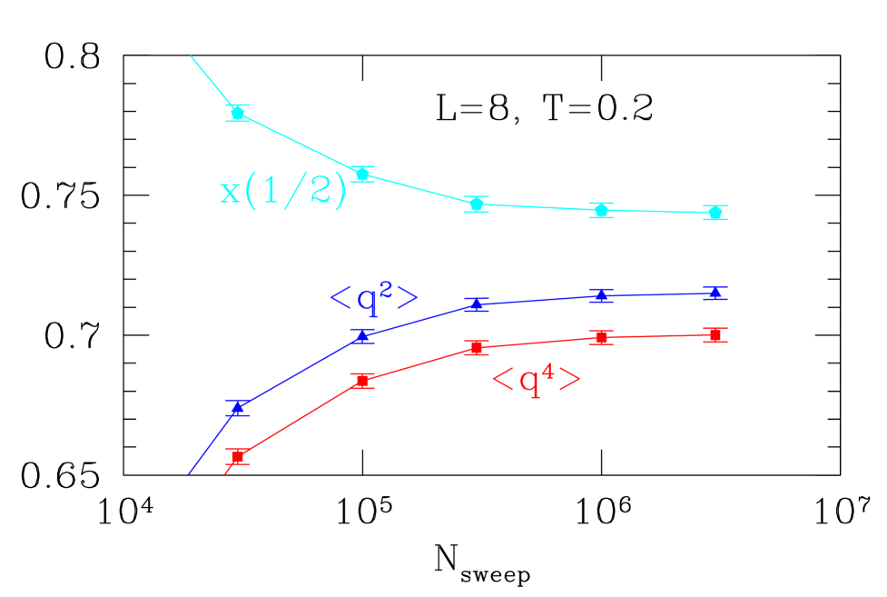
FIG. 1.: An equilibration plot for $L=8,T=0.20$, for the second and fourth moment of $P(q)$, and for $x(1/2)$, the average of $P(q)$ over the interval $|q|\leq 1/2$. For better viewing, the data for $\langle q^{4}\rangle$ and $x(1/2)$ have been shifted upwards by 0.14 and 0.67, respectively. For each value of $N_{sweep}$, the averages were measured over the last $N_{sweep}/3$ MC sweeps.

Simulations of spin glasses at very low temperatures are now possible, at least for modest sizes, using the parallel tempering Monte Carlo method[17, 18], where one simulates replicas of the system at $N_{T}$ different temperatures. Here, we need two copies of the system at each temperature to calculate $q$, so we actually run 2 sets of $N_{T}$ replicas. We also gain a large speed-up by using multispin coding[19] to store each spin or bond as a single bit rather than a whole word.

In earlier work[3] for the Gaussian distribution we were able to use a special relationship between certain variables to check for equilibration, but this is not applicable here. We therefore investigate whether various quantities have become independent of simulation time when plotted on a logarithmic scale. Fig. 1 shows an example for $L=8,T=0.20$ indicating that the data seems to have saturated.

L	$N_{\mathrm{samp}}$	$N_{\mathrm{sweep}}$	$N_{T}$	$T_{min}$
4	9600	$10^{5}$	15	0.05
6	6400	$10^{6}$	15	0.05
8	3904(∗)	3 $\times 10^{6}$	21	0.2
10	1408	$10^{7}$	19	0.35

TABLE I.: Parameters of the simulations. $N_{\mathrm{samp}}$ is the number of samples (i.e. sets of bonds), $N_{\mathrm{sweep}}$ is the total number of sweeps simulated for each of the $2N_{T}$ replicas for a single sample, $N_{T}$ is the number of temperatures used in the parallel tempering method, and $T_{min}$ is the lowest temperature simulated. ^(∗) $N_{\mathrm{samp}}$=6336 for $L=8$ and $T\geq 0.35$.

In Table I, we show the simulation parameters. The lowest temperature simulated, $T_{min}$, has to be compared with[20] $T_{c}\approx 1.15$. For each size the largest temperature is 2.0. The set of temperatures is determined by requiring that the acceptance ratio for global moves is 0.3 or larger.

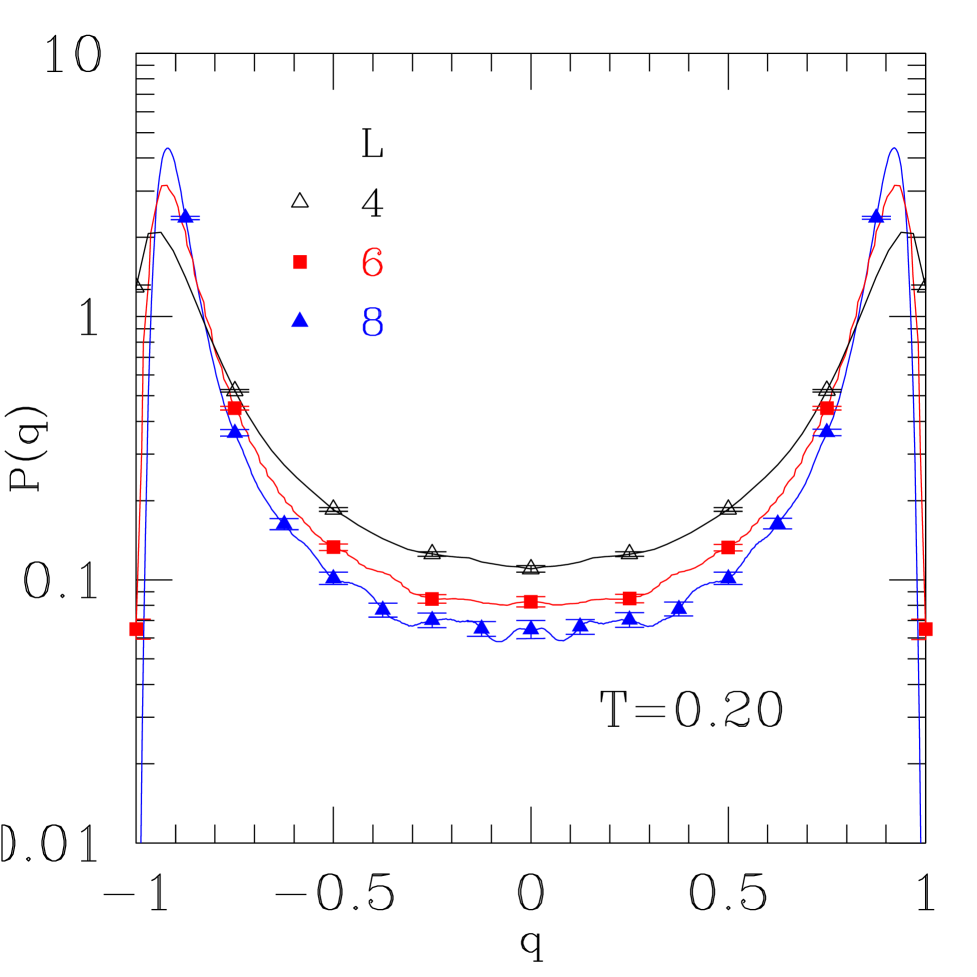
FIG. 2.: Data for the overlap distribution $P(q)$ at $T=0.20$. The vertical scale is logarithmic to better make visible the peak at large $q$ and the tail down to $q=0$. We only display some of the data points as symbols, for clarity, but the lines connect all the data points. This accounts for the curvature between neighboring symbols.

Figs. 2 and 3 show data for $P(q)$ for different sizes at $T=0.2$ and $T=0.35$. One can see that the weight in the tail tends to decrease initially with increasing $L$, especially at lower $T$, but for $T=0.35$ the data seems to saturate at larger $L$. For $T=0.5$ (not displayed) the weight in the tail saturates already at $L=4$. This can be seen more clearly in Fig. 4, which shows $x(1/2)$ as a function of $L$ for different temperatures, where $x(q)=\int_{-q}^{q}P(q^{\prime})dq^{\prime}$ so $x(1/2)$ is the average of $P(q)$ from $-1/2$ to $1/2$. We give data for $x(1/2)$ rather than $P(0)$ because the statistics are better and also so we can compare directly with other work. For $L=4$ and $L=6$, the data at $T=0.05$, not showed in Fig. 4, are superimposed to the data at $T=0.2$, indicating that we have reached the true $T=0$ behavior. For $L=8$, the data at $T=0.2$ may be one or two standard deviations larger than the $T=0$ value. Furthermore, the average energy at $T=0.2$ agrees with the ground state results by Pal[21]. From a power law fit of the data in Fig. 4 at $T=0.2$ we estimate

$$\lambda=0.9\pm 0.1\,.$$ (3)

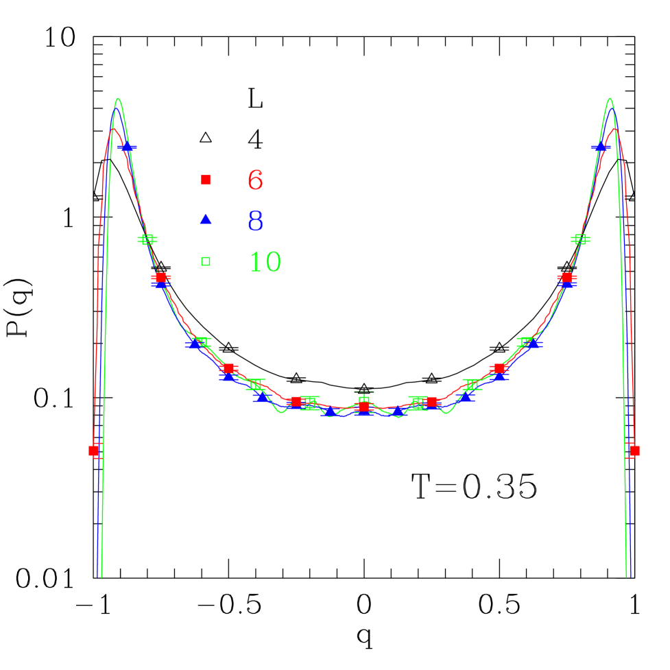
FIG. 3.: Same as for Fig. 2 but at $T=0.35$.

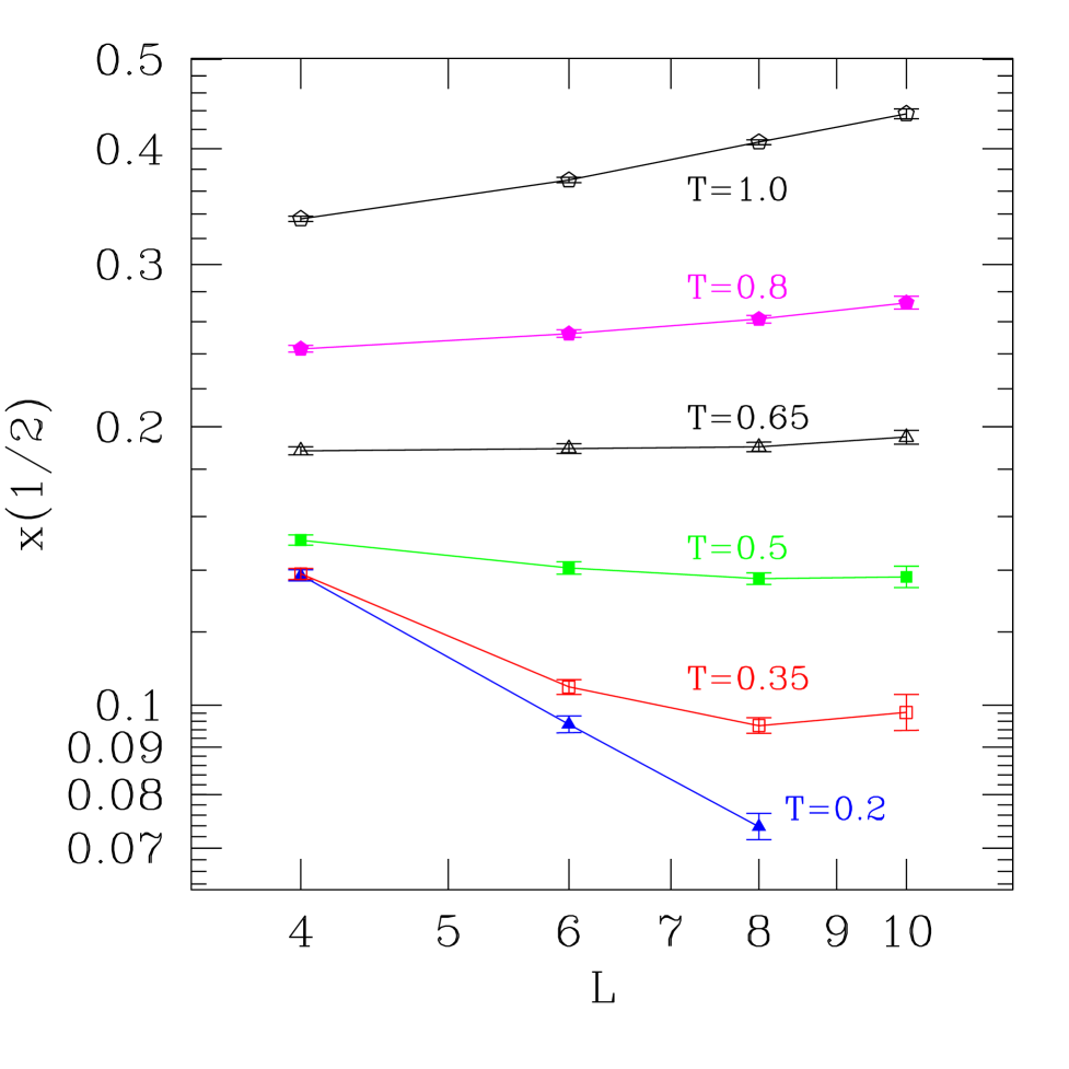
FIG. 4.: Log-log plot of $x(1/2)$, the average of $P(q)$ over $|q|\leq 1/2$, against $L$.

Generalizing the KM argument to a scenario described by an exponent $\theta$, we expect that at finite-$T$ there will be a crossover between the $L^{-(\lambda+\theta)}$ behavior for $L$ smaller than some length scale $L_{c}(T)$, and the $L^{-\theta}$ behavior (or, for $\theta=0$, an $L$-independent value proportional to $T$), at scales larger than $L_{c}(T)$. In the more general case, assuming scaling one has $L_{c}(T)\sim T^{-1/\lambda}$ and

$$x(1/2)=TL^{-\theta}f(LT^{1/\lambda}),$$ (4)

where $f$ is a scaling function.

A scaling plot appropriate to this behavior, for $\theta=0$ and $\lambda=0.9$, is shown in Fig. 5, where one can see that the data collapse fairly well. The data in Fig. 4 increase with increasing $L$ for $T\geq 0.8$, due to the vicinity of $T_{c}$, where $x(1/2)\sim L^{\beta/\nu}$ and[20] $\beta/\nu\simeq 0.3$. One may therefore argue[22] that the observed saturation between $T=0.35$ and $T=0.65$ is a finite size effect and that at larger sizes there will be a second crossover to the $L^{-\theta}$ behavior. We cannot exclude this possibility, though we note that $T=0.35$ is quite far from $T_{c}$ and that a scaling plot as in Fig. 5 but with $\theta=0.2$ is significantly worse.

Hartmann[13] computed $x(1/2)$ as a function of $L$ at zero temperature and found that a power law fits well the data with an exponent $\lambda=1.25\pm 0.05$, which disagrees with our estimate. Our value for $\lambda$ does, however, agree with that of Berg et al.[10] who find $\lambda=0.72\pm 0.12$. In addition, our raw data for $x(1/2)$ is consistent with (though more accurate than) that of Berg et al.[10], but is inconsistent with that of Hartmann[13] for $L>4$. For example, for $L=6$ we find $x(1/2)=0.095\pm 0.002$, while Hartmann finds $x(1/2)=0.083\pm 0.005$. We note however that Hartmann’s method, unlike (properly equilibrated) Monte Carlo simulations, is not guaranteed to sample all the ground states with equal probability.

Our results for $P(q)$ at low-T are also in marked disagreement with HG. For example, HG report a $P(q)$ which is lower than $0.03$ in the interval $|q|\leq 0.1$ for $L=8$ and $T=0.3$, while our average of $P(q)$ over this interval is between $0.066\pm 0.004$ (our value at $T=0.275$) and $0.081\pm 0.004$ (our value $T=0.35$). HG observe a pronounced decrease of $P(q)$ with $L$ even at $T=0.5$, where our data clearly saturate. We also computed the Binder cumulant, which agrees with Ref. [15] but disagrees with HG. This suggests that the simulations of HG are not correctly equilibrated, as discussed in detail in Ref. [15].

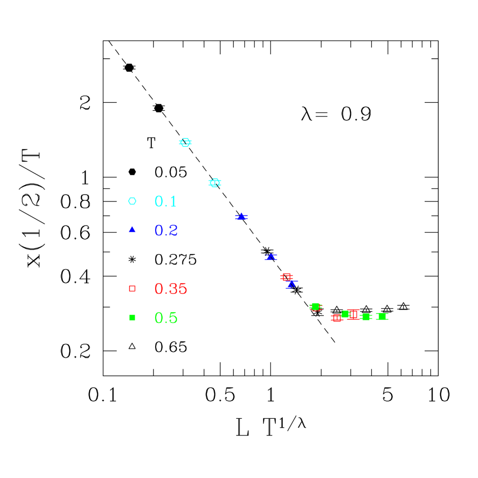
FIG. 5.: The scaling behavior of $x(1/2)$ expected from Eq. (4) with $\theta=0$. For $L\gg L_{c}(T)\sim T^{-1/\lambda}$, $x(1/2)$ is independent of size, while for $L\ll L_{c}(T),x(1/2)$ varies as $L^{-\lambda}$. The dashed line has a slope of $-0.9$.

KM give arguments that $\lambda$ should equal $d_{s}/2$ where $d_{s}$ is the fractal dimension of the surface of the large-scale low-energy excitations which give rise to a nontrivial energy landscape. However, one expects that $d_{s}\geq d-1$ which is barely satisfied by the estimate in Eq. (3) which corresponds to $d_{s}=1.8\pm 0.2$. Furthermore, for the Gaussian distribution, $d_{s}$ is significantly larger than this value. For example, Ref. [2] finds $d_{s}=2.58\pm 0.02$. While it is possible that $d_{s}$ could be different for the Gaussian and $\pm J$ models, our results suggest that $\lambda\neq d_{s}/2$, and that there may be corrections to the argument of KM.

To conclude, results from simulations on small sizes indicate that the order parameter distribution of the $\pm J$ Ising spin glass is trivial at $T=0$ but, at least for quite small sizes, is nontrivial at finite-$T$ in agreement with the conclusions of KM. We have also demonstrated crossover scaling between the zero-$T$ and finite-$T$ behaviors. We expect similar results in other models with a discrete disorder distribution, and indeed this is what we find in preliminary unpublished data for the $\pm J$ Ising spin glass in $d=4$. Whether these conclusions are still valid in the thermodynamic limit remains an open question. However, we emphasize, quite generally, that a trivial $P(q)$ at $T=0$ does not, in itself, imply evidence for the droplet model since this is also expected if $P(q)$ is nontrivial at finite-$T$, as pointed out by KM.

After this work was submitted we received a paper by Hed et al.[23], in which, based on a different analysis from ours, they claim that $P(q)$ is non-trivial at $T=0$.

This work was supported by the National Science Foundation under grant DMR 0086287. The numerical calculations were made possible by a grant of time from the National Partnership for Advanced Computational Infrastructure. We should also like to thank A. Hartmann for helpful correspondence.

REFERENCES

- [1] F. Krzakala and O. C. Martin, Phys. Rev. Lett. 85, 3013 (2000), cond-mat/0002055
- [2] M. Palassini and A. P. Young, Phys. Rev. Lett. 85, 3017 (2000), cond-mat/0002134.
- [3] H. G. Katzgraber, M. Palassini and A. P. Young, cond-mat/0007113.
- [4] E. Marinari and G. Parisi, cond-mat/0007493.
- [5] We make no comments here as to whether these conclusions will still be valid in the thermodynamic limit.
- [6] G. Parisi, Phys. Rev. Lett. 43, 1754 (1979); J. Phys. A 13, 1101, 1887, L115 (1980); Phys. Rev. Lett. 50, 1946 (1983).
- [7] D. S. Fisher and D. A. Huse, J. Phys. A. 20 L997 (1987); D. A. Huse and D. S. Fisher, J. Phys. A. 20 L1005 (1987); D. S. Fisher and D. A. Huse, Phys. Rev. B 38 386 (1988).
- [8] A. J. Bray and M. A. Moore, in Heidelberg Colloquium on Glassy Dynamics and Optimization, L. Van Hemmen and I. Morgenstern eds. (Springer-Verlag, Heidelberg, 1986).
- [9] F. Krzakala and O. C. Martin, cond-mat/0010010 (referred to as KM).
- [10] B. A. Berg, U. E. Hansmann and T. Celik, Phys. Rev. B 50, 16444 (1994).
- [11] A. K. Hartmann, Europhys. Lett. 40, 429 (1997).
- [12] A. Sandvik, Europhys. Lett. 45, 745 (1999).
- [13] A. K. Hartmann, Euro. Phys. Jour. B 13 539 (2000).
- [14] N. Hatano and J. E. Gubernatis, cond-mat/0008115 (referred to as HG).
- [15] E. Marinari, G. Parisi, F. Ricci-Tersenghi and F. Zuliani, cond-mat/0011039.
- [16] G. Hed, A. K. Hartmann, D. Stauffer and E. Domany, cond-mat/0007356.
- [17] K. Hukushima and K. Nemoto, J. Phys. Soc. Japan 65, 1604 (1996).
- [18] E. Marinari, Advances in Computer Simulation, edited by J. Kertész and Imre Kondor (Springer-Verlag, Berlin 1998), p. 50, (cond-mat/9612010).
- [19] N. Kawashima, N. Ito and Y. Kanada, Int. J. Mod. Phys. C 4, 525 (1993).
- [20] H. G. Ballesteros et al., cond-mat/0006211; M. Palassini and S. Caracciolo, Phys. Rev. Lett. 82, 5128 (1999); N. Kawashima and A. P. Young, Phys. Rev. B 53, R484 (1996); B. A. Berg and W. Janke, Phys. Rev. Lett. 80, 4771 (1998).
- [21] K. F. Pal, Physica A 223, 283 (1996).
- [22] M.A. Moore, H. Bokil and B. Drossel, Phys. Rev. Lett. 81, 4252 (1998); B. Drossel, H. Bokil, M.A. Moore and A.J. Bray, Eur. Phys. J. B 13, 369 (2000); H. Bokil, B. Drossel and M.A. Moore, Phys. Rev. B 62, 946 (2000).
- [23] G. Hed, A. K. Hartmann, and E. Domany, cond-mat/0012451.