Spin Tunneling in Molecular Magnets

Abstract

We study spin tunneling in magnetic molecules, with special reference to Fe₈. The article aims to give a pedagogical discussion of what is meant by the tunneling of a spin, and how tunneling amplitudes or energy level splittings may be calculated using path integral and discrete phase integral methods. In the case of Fe₈, an issue of great interest is the oscillatory tunnel splittings as a function of applied magnetic field that have recently been observed. These oscillations are due to the occurrence of diabolical points in the magnetic field space. It is shown how this effect comes about in both the path-integral and the discrete phase integral methods. In the former it arises due to the presence of a Berry-like phase in the action, which gives rise to an interference between tunneling trajectories. In the latter, it arises due to the presence of further neighbor terms in the recursion relation for the energy eigenfunction. These terms give rise to turning points which have no analog in the one-dimensional continuum quasiclassical method. Explicit results are obtained for the location of the diabolical points in Fe₈.

I Introduction

Tunneling is a basic way in which the difference between quantum and classical mechanics manifests itself, and even though the simplest examples of tunneling were studied right after the birth of quantum mechanics, there are many other aspects of tunneling that are still the subject of active research today. It is generally quite difficult to calculate tunnel splittings in many particle systems, and even for one particle, the step from one to two spatial dimensions presents significant challenges and surprises [2, 3].

In this article, I shall study the tunneling of a single spin degree of freedom. This is yet another instance where the statement of the problem is very simple, yet the earliest study of which I am aware dates to 1978[4], a half-century after the founding of modern quantum theory.

From the point of view of this volume, the greatest interest in spin tunneling lies in the possibility of observing meso or macroscopic quantum phenomena (MQP) in magnetic particles and related systems, as first proposed in the late 1980’s [5, 6]. The range of activity over the next half-decade is well represented in a workshop proceedings [7]. After preliminary investigation, small magnetic particles appear to be attractive candidates for MQP, since for diameters $\sim 50$ Å, and typical anisotropy constants, the tunneling rates appear to be moderately large. However, in contrast to the situation that prevails in the SQUID systems (for which, see the article by Han in this volume), it turns out that the classical dynamics of the net magnetic moment of a small particle is not fully understood theoretically, especially with regard to dissipation. On the experimental side, the characterization and reproducible fabrication of very small particles is still rather difficult, and at present even the measurement and modeling of the classical dynamics is not a fully solved problem. Wernsdorfer’s article in this volume gives a good sense of the issues involved. It is this author’s opinion (which is not necessarily shared widely), that unless the classical dynamics is fully understood, theoretical analyses are not likely to be pertinent, and the interpretation of experiments will be uncertain.

In the last few years, however, a much more fruitful avenue for the spin tunneling has opened up in the area of large magnetic molecules. Several dozen molecules are presently under study, but the two that have yielded the most fruitful results are Mn₁₂ and Fe₈. In this author’s view, which is again not necessarily held by the majority of workers in the field, the hysteresis phenomena seen in Mn₁₂ to date[8, 9, 10] (c.f. review by Friedman in this volume) are not due to spin tunneling alone, but reflect a much richer and more complex many-body effect originating in the spin-phonon interaction [11, 12]. In the case of Fe₈, however, there is unambiguous evidence of spin tunneling in the form of an oscillatory magnetic field dependence of the tunnel splitting, as seen by Wernsdorfer and Sessoli [13]. This dependence is highly systematic, and not easy to obtain by accident, so as an experimental signature it is very robust. Theoretically, these oscillations represent a very interesting difference between spin and massive particles. This difference can be attributed almost tautologically to the difference in the commutation relations. A much more visual representation of the difference is provided by the difference in path integrals between these systems. The spin path integral contains a kinetic term which has the properties of a Berry phase, which can give rise to interference between different spin trajectories [14, 15]. The oscillations are a result of such an interference effect, and were in fact predicted theoretically without knowing of the relevance of the work to Fe₈ [16]. Very briefly, here is how the effect arises. The classical state of a spin is defined by giving its orientation ${\bf{\hat{n}}}$, and the paths lie on the surface of a unit sphere. The sum over paths is dominated by least action paths, or instantons. For certain field orientations, one finds that there are two such least action paths that wind around ${\bf H}$ in opposite directions (Fig. 1). The real part $S_{R}$ of the Euclidean action is equal for both paths, but the imaginary parts differ, giving rise to a relative phase equal to the Berry phase for the closed loop formed by the two paths. This Berry-phase is proportional to the area $\Omega$ of the loop. Thus, the splitting $\Delta$ is given by

$$\Delta\propto\exp(-S_{R})\cos\Phi,$$ (1)

where $\Phi=J\Omega/2$, with $J$ being the magnitude of the spin. As the field is increased, the minima between which the instantons run move toward each other, and the area $\Omega$ shrinks. Whenever $\Phi$ passes through an odd multiple of $\pi/2$, $\Delta$ vanishes. In Fig. 1, we also show the result of a direct numerical computation of $\Delta$ as a function of $H$ for the model Hamiltonian used in Ref. [16], showing that the effect is real.

FIG. 1.: Interfering instanton trajectories, and numerically computed $-10\leftrightarrow+10$ tunnel splitting for a model for Fe₈ with ${\bf H}\|{\bf{\hat{x}}}$.

However, a proper discussion of spin path integrals requires the development of a fair amount of calculational machinery, which is not part of the standard repertoire of most physicists despite having been around for almost 25 years [17, 18]. Indeed, in discussions with non-experts this author has found that several more elementary issues need to be clarified first. Further, path integrals are just one way to calculate tunnel splittings. In analogy with massive particles, there is also a phase integral or WKB method [19, 20, 21, 22, 23, 24] that can be applied to spin. For some calculational purposes, this is in fact superior to the path integral approach. Unfortunately, this method is also not standard textbook material, and while it involves far more elementary mathematics than the path integrals do, again, a fair amount of machinery must be developed before it can be used efficiently.

In this article, I shall (among other things) try and give a simple treatment of both the path integral and discrete phase integral methods. In order to orient this discussion, however, it is first necessary to go back and ask what we mean by spin tunneling to begin with. To this end, let us consider the toy Hamiltonian

$${\cal H}_{\rm toy}=k_{1}J_{x}^{2}+k_{2}J_{y}^{2},$$ (2)

with $k_{1}>k_{2}>0$. ${\bf J}$ is a dimensionless spin operator with the usual commutation rules:

$$[J_{i},J_{j}]=i\epsilon_{ijk}J_{k}.$$ (3)

The first step is to understand the classical version of this problem. What is the configuration space, the phase space, how are the classical dynamics to be defined, and what are the classical states between which tunneling will take place when quantum mechanics is turned on? To answer these questions, we first note that a classical angular momentum (which we also denote by ${\bf J}$) obeys the Poisson brackets

$$\{J_{i},J_{j}\}_{\rm PB}=\epsilon_{ijk}J_{k}.$$ (4)

Thus we can regard Eq. (2) as a classical Hamiltonian (with the dimensions of ${\bf J}$ and the $k$’s suitably readjusted), which defines the dynamics of the vector ${\bf J}$ through the Poisson brackets (4):

$${d{\bf J}\over dt}=\{{\bf J},{\cal H}\}_{\rm PB}=-{\bf J}\times{\partial{\cal H}\over\partial{\bf J}}.$$ (5)

In fact, it is clear that (5) is a general prescription applicable to any Hamiltonian that is a function of the components of ${\bf J}$ only. An immediate consequence of Eq. (5) is that

$${d\over dt}{\bf J}\cdot{\bf J}=-2{\bf J}\cdot\left({\bf J}\times{\partial{\cal H}\over\partial{\bf J}}\right)=0,$$ (6)

so $|{\bf J}|$ is a constant of the motion, and configurations are completely specified by giving the orientation ${\bf{\hat{J}}}={\bf J}/|{\bf J}|$, and the configuration space is the unit sphere. At the same time, once ${\bf{\hat{J}}}$ is specified at any given time $t=0$, Eq. (5) allows us to find it uniquely at any later time $t>0$, as it is a first order differential equation for ${\bf{\hat{J}}}$. Thus the unit sphere is a carrier manifold in the language of modern classical mechanics, and it is also the phase space. In other words, for spin, configuration and phase space are one and the same.

If we interpret Eq. (2) as a classical Hamiltonian, then the classical energy minima arise when ${\bf J}=\pm J{\bf{\hat{z}}}$. These minima are degenerate. When the problem is made quantum mechanical, these two classical states will appear as two energy eigenstates with a small tunneling induced splitting. The problem can be approached in two stages. First of all, classical states with definite values of ${\bf J}$ go over into quantum mechanical states in which ${\bf J}$ automatically has a spread since the components of ${\bf J}$ do not commute. The states with ${\bf J}=\pm J{\bf{\hat{z}}}$ will acquire a zero point spread $\langle J_{x}^{2}\rangle\sim\langle J_{y}^{2}\rangle\sim J$. (One can easily find these states by solving and quantizing the equations of motion in the harmonic approximation. This is completely equivalent to the Holstein-Primakoff procedure.) In the second stage, tunneling mixes these states.

With this preamble, we can pose the basic question. What is the tunnel splitting for a Hamiltonian such as (2) which has two (or more) degenerate classical minima? In the course of answering this question, other questions arise fairly quickly. For example, from a purely theoretical or mathematical perspective, what are the associated wave functions? What are the splittings between excited pairs of levels? The answers to these can be sought at varying levels of rigour and quantitative accuracy. From the perspective of making contact with experiments, one may want to know the influence of various perturbations and “dirt effects”. Here, an important distinction needs to be made between static and dynamic perturbations. For static perturbations, the problem reduces to finding the matrix elements of various operators between the tunneling states. The number of important operators in any system is generally not large, so this type of question can be moved over into the theory column in some sense. For time dependent perturbations, two further subclasses need to be recognized. If the time dependence is of the c-number type, i.e. due to a time-varying external field, the problem can be reduced to either a standard NMR type, or to a Landau-Zener-Stückelberg type. If the perturbation is due to other dynamical degrees of freedom, however, the problem is much harder, and is in fact conceptually the same as that in investigations of dissipation and decoherence in MQP. The range of possibilities here is quite large in general, but in molecular magnetic systems one has the advantage of knowing the relevant environmental degrees of freedom with a high level of confidence, which greatly aids in theoretical modeling.

In this article, we shall largely be concerned with the theoretical aspects of the problem. For specificity, we will focus on the Fe₈ system, but the methodology is completely general. In Sec. II, we will review the salient features of the Fe₈ system, and discuss the results of the Wernsdorfer and Sessoli experiment, with emphasis on the oscillatory field dependence and vanishing of the tunnel splitting. We will compare these results with numerical studies of the simplest model Hamiltonian for Fe₈, consider the points where the splittings vanish in light of general quantum mechanical theorems about degeneracy, and see that these points form a very rich pattern in the magnetic field space.

In Sec. III, we will turn to the spin-coherent-state path integral approach. These path integrals are much more delicate than the Feynman integral for a massive particle, and the mathematical subtleties of the semi-classical limit are still being researched. We will sidestep these points, and concentrate on the Berry phase and the quenching condition for the special case where the magnetic field is along the hard magnetic axis of the molecule [16]. This is the simplest case, and corresponds to a symmetric double well problem. When the field is not along the hard or easy exes, the problem does not have any symmetry, and instanton calculations, though possible, are quite involved. More quantitative calculations can be done with comparatively greater ease using a discrete phase integral (or WKB) method. We will discuss the basic idea behind this method, and then show how this method can be used to find tunnel splittings for Fe₈ for all orientations of magnetic field [25, 26, 27, 28].

II The Fe₈ system

A Summary of experimental facts and spin model

The molecule Fe₈ (proper chemical formula: [Fe₈O₂(OH)₁₂(tacn)₆]⁸⁺) is magnetic, and

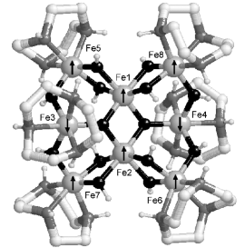
FIG. 2.: The Fe₈ molecule.

forms good single crystals. It has an approximate D₂ symmetry (see Fig. 2). In its lowest state, it is found to have a total spin of 10, arising from competing antiferromagnetic interactions between the Fe³⁺ ions within a molecule. Spin-orbit and spin-spin interactions destroy complete rotational invariance, and give rise to an anisotropy with respect to the crystal lattice directions. A variety of experimental techniques (electron spin resonance, ac susceptibility, magnetic relaxation, Mössbauer spectroscopy, neutron scattering) indicates [29, 30, 31, 32, 33] that a single molecule can be described by the Hamiltonian

$${\cal H}_{0}=k_{1}J_{x}^{2}+k_{2}J_{y}^{2}-g\mu_{B}{\bf J}\cdot{\bf H},$$ (7)

with $J=10$, $k_{1}\approx 0.33\$K, and $k_{2}\approx 0.22\$K. In addition, there are much weaker higher order anisotropies. The leading fourth order anisotropy correction is

$${\cal H}_{4}=-k_{4}(J_{+}^{4}+J_{-}^{4}),$$ (8)

with $k_{4}\approx 2.9\times 10^{-5}\$K [13]. The anisotropy energy is equivalent to a field of $\sim 2.5\$T. The $g$ factor is very close to 2.

In writing the Hamiltonian for the eight coupled Fe³⁺ spins in terms of a single total spin ${\bf J}$ as we have done, the chief assumption is that other spin multiplets are well separated in energy from the ground multiplet. It is very hard to do first principles calculations of the intramolecular, interionic exchange parameters, and even when one can do this, it is very hard to diagonalize the resulting Heisenberg exchange Hamiltonian. EPR experiments do not show any evidence of other multiplets, and so while a definite number is not known, it is not unreasonable to guess that other multiplets will be separated from the $J=10$ ground multiplet by at least tens of Kelvin. Especially for the tunneling, the other multiplets can be safely ignored.

Let us also briefly discuss environmental degrees of freedom which have been left out of the description (7), and their interaction with the spin. First, different molecules may interact with each other. However, the Fe₈ molecule is very large, and in the solid, so is the intermolecular separation. The primary interaction between molecules is dipolar (there is no intermolecular exchange, in particular), and the dipolar field on any molecule is about 100 Oe [34], much weaker than the intramolecular anisotropy field. Second, there is a spin-phonon interaction, which as in the case of Mn₁₂, is responsible for the moderate to high temperature magnetization relaxation [31], and the dramatic hysteresis loop steps [32] seen in this molecule too. At low temperatures, however, very few phonons are present in equilibrium, and to a first approximation they may be neglected. This is especially so for the tunneling phenomena we will consider in this article. Third, the atomic spins couple to the nuclear spins–the hyperfine interaction. The biggest such coupling comes from magnetic nuclei in the magnetic species. For iron, the only isotope with a magnetic nucleus is ⁵⁷Fe, with a natural abundance of 2-2.5%. Thus, about 75% of the molecules have no nuclear spin in the magnetic species at all, and for those that do, the hyperfine field seen by the electronic spin is about 10-100 Oe. If we average the hyperfine field, and lump this along with the dipolar field in the form of an inhomogeneous field, we get a distribution with a width of about 200 Oe [34], far smaller than the anisotropy field. (Alternatively, we could say that the energy scales associated with dipolar plus hyperfine interactions and the magnetic anisotropy are 0.2 K and 25 K, respectively.) This approximation omits the dynamical aspects of the nuclear spins, which are expected to give rise to a small unquenching of the spin tunneling, i.e., make the transition probability nonzero. Thus, this aspect of the problem is potentially important for a detailed understanding of the Wernsdorfer-Sessoli data, as is the distribution of dipolar and hyperfine fields.

In the rest of this article, we shall only study the pure spin problem described by Eq. (7) and (8). Further, for the most part, we shall ignore the fourth order correction (8). This term is important in that even though it is a small correction to the energy of any state, it significantly modifies the location of the points in the magnetic field space where the splitting vanishes. For the conceptual problem of understanding why we get a vanishing splitting in the first place, however, it is sufficient to study only ${\cal H}_{0}$. We shall discuss the effects of including ${\cal H}_{4}$ is Sec. II D briefly.

B Tunneling states and the Landau-Zener-Stuc̈kelberg process

If ${\bf H}=0$, ${\cal H}_{0}$ is exactly the toy model of Sec. I, and there are two degenerate energy minima at $\pm{\bf{\hat{z}}}$. If ${\bf H}\neq 0$, but still in the xy plane, the classical minima move off the $\pm{\bf{\hat{z}}}$ directions but continue to be degenerate. One way to understand the tunneling between these directions is to rewrite Eq. (7) after subtracting out a constant term $k_{2}{\bf J}\cdot{\bf J}=k_{2}J(J+1)$, and explicitly putting $H_{z}=0$. This yields

$${\cal H}=-k_{2}J_{z}^{2}+(k_{1}-k_{2})J_{x}^{2}-g\mu_{B}(J_{x}H_{x}+J_{y}H_{y}).$$ (9)

Let us now regard the last three terms as perturbations that give rise to transitions between various Zeeman levels or eigenstates of $J_{z}$. As usual, we denote the $J_{z}$ value by $m$. The $J_{x}^{2}$ term gives rise to $\Delta m=2$ transitions, and thus mixes $m=-10$ with $m=+10$ via the $-8$, $-6$, $\ldots$, $+8$ states. The $H_{x}$ and $H_{y}$ terms give rise to $\Delta m=1$ transitions, and mix $m=-10$ with $+10$ via all intermediate levels $-9$ to $+9$ (see Fig. 3a). This picture allows us to think of spin tunneling in direct analogy with a particle tunneling through an energy barrier. It is further obvious that if we also apply a field along the $z$ direction so as to tune the energies of the $-10$ and $+9$ states to resonance, we can also think of tunneling between these states. More generally, we can consider tunneling between a state with $m=m_{i}$ on the negative $m$ side and $m=m_{f}$ on the positive $m$ side.

FIG. 3.: (a) Zeeman levels of Fe₈, showing $\Delta m=1$ (solid lines) and $\Delta m=2$ (dashed lines) transitions. (b) The Landau-Zener-Stückelberg process.

At this point, it is appropriate to ask if the tunnel splitting is big enough to measure experimentally. Although one of the main goals of this article is to understand such splittings analytically, let us temporarily cheat and diagonalize the $21\times 21$ Hamiltonian matrix numerically with the experimental numbers for $k_{1}$ and $k_{2}$. When this is done, we find that the splitting, $\Delta\sim 10^{-8}$ K. We now recall that the bias or departure from degeneracy between the $m=\pm 10$ states caused by the dipolar and hyperfine fields, which we denote by $\epsilon$, is about 0.1 K, which is enormous compared to $\Delta$. Hence, left to itself, a spin will have almost no chance of tunneling at all. To see this, consider a two level Hamiltonian

$$\left(\begin{array}[]{cc}\epsilon&\Delta\\ -\Delta&-\epsilon\end{array}\right).$$ (10)

It is now easy to verify that if we start at $t=0$ in the $+\epsilon$ level, the probability of finding the system in the $-\epsilon$ level at a later time oscillates with a frequency, $2(\Delta^{2}+\epsilon^{2})^{1/2}$, and an amplitude $\Delta^{2}/(\Delta^{2}+\epsilon^{2})$. If $\epsilon\gg\Delta$, the transition probability is always very small. The same general conclusions apply to any two levels $m_{i}$ and $m_{f}$, not just the $\pm 10$ states.

Wernsdorfer and Sessoli solve this difficulty by making use of the Landau-Zener-Stückelberg (LZS) mechanism to induce tunneling transitions[35]. A dc longitudinal field $H_{z}$ is applied so as to bring $m_{i}$ and $m_{f}$ into approximate resonance. They then apply an additional ac longitudinal magnetic field $H_{z}(t)$ in the form of a triangular wave. Denoting the amplitude of this wave by $H_{0}$ and the time period by $\tau$, we have $\dot{H}=|dH_{z}/dt|=4H_{0}/\tau$. Now, as $H_{z}$ changes with time, the energies of the $-10$ and $+10$ levels will move in opposite directions, and at some point in the cycle they will cross. (See Fig. 3b.) This gives rise to what is known as the LZS process. Basically, in the vicinity of the crossing, the energy bias goes to zero, and there is an appreciable chance for the spin to tunnel. The probability for a transition during one crossing is given by [36]

$$P=1-e^{-\gamma},$$ (11)

where

$$\gamma={2\pi\Delta^{2}\over(g\mu_{B}\hbar)\Delta m\dot{H}},$$ (12)

and $\Delta m=|m_{f}-m_{i}|$ is the change in $m$ in the transition. The quantity $\gamma$ is known as the adiabaticity parameter, and in the limit where the crossing is passed rapidly, i.e., $\dot{H}$ is large, $\gamma\ll 1$, and $P\approx\gamma$. We can further assume that because the stray fields are fluctuating, the phase of the molecule will be randomized and uncorrelated between successive crossings. If $H_{0}$ is large enough to overcome the range of dipolar biases (but not so large as to make more than one Zeeman level on the positive side cross the level on the negative side), every molecule in the sample will undergo a crossing at some point in the cycle. Since there are $2/\tau$ crossings per unit time, we obtain a transition probability per unit time for $m_{i}\leftrightarrow m_{f}$ transitions, given by

$$\Gamma_{\rm LZS}={2\over\tau}\gamma\approx{\pi\Delta^{2}\over(g\mu_{B}\hbar)\Delta mH_{0}}\quad(\gamma\ll 1).$$ (13)

Wernsdorfer and Sessoli first saturate the sample in a large longitudinal field. This field is then removed and the ac field is applied, inducing LZS transitions, and causing a relaxation of the magnetization of the sample. By measuring the rate of this relaxation, one can obtain $\Gamma_{\rm LZS}$, from which one can in turn infer $\Delta$ using Eq. (13) and the experimental value of $H_{0}$. An important check on the consistency of the LZS interpretation implied by Eq. (13) is that the relaxation rate should be independent of the sweeping rate $\dot{H}$. Experimentally, this is found to be true for $\dot{H}$ ranging from 1 mT/s to 1 T/s.

C Oscillatory tunnel splittings, the von Neumann-Wigner theorem, and diabolical points

It is apparent that the LZS measurements can be carried out in the presence of a transverse dc field (in the xy plane) $H_{\perp}$, so that $\Delta$ can be measured as a function of $H_{\perp}$. Naively, we expect that since increasing $H_{\perp}$ decreases both the energy barrier and the angle through which the spin must tunnel, $\Delta$ will increase monotonically with $H_{\perp}$. What is actually seen

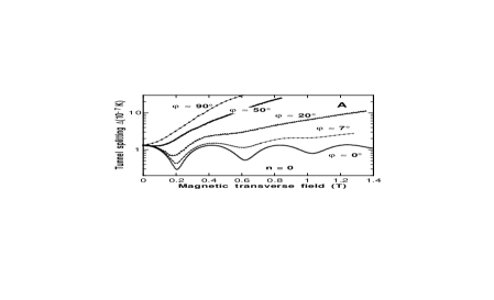
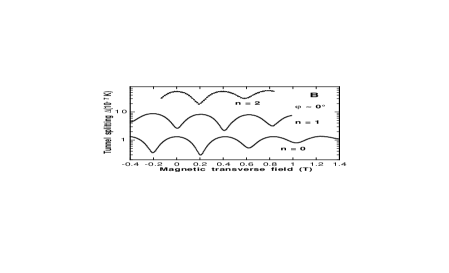
FIG. 4.: Measured splittings [12] for Fe₈ for (a) $-10\leftrightarrow 10$ transitions for various orientations of ${\bf H}$ in the xy plane, and (b) for ${\bf H}\|{\bf{\hat{x}}}$ between the states $m=-10$ and $m=10-n$.

experimentally is rather different (see Fig. 4). When ${\bf H}\|{\bf{\hat{y}}}$ ($\phi=90^{\circ}$), the behavior is indeed monotonic, but when ${\bf H}\|{\bf{\hat{x}}}$, one finds that $\Delta$ oscillates with $H_{x}$.

We have already stated in Sec. I that this oscillation can be understood in terms of a Berry phase in the spin path integral. Since the vanishing of $\Delta$ means that two energy levels of the system are exactly degenerate, it is useful to examine this result in general quantum mechanical terms, and from the perspective of rigorous results about when such degeneracies can and cannot occur. Before we turn to this, however, it is useful to look at the results of a numerical diagonalization of the Hamiltonian (7). These numerical data reveal a number of other properties, some of which are special to the form (7), but others are general. In Fig. 5, we show the results of numerical calculation of the energies as a function of $H_{x}$, for

FIG. 5.: Spectrum of the Hamiltonian (2.1) for $J=3$, as a function of $H_{x}/H_{c}$, with $H_{c}=2k_{1}J/g\mu_{B}$. $H_{z}/H_{c}=0$, $0.07454$, and $0.1491$ in (a), (b), and (c), respectively. The small ovals indicate narrowly avoided anticrossings that appear to be crossings on the resolution of this figure.

$J=3$, for three different values of $H_{z}$. In all three cases, $H_{y}=0$. In part (a), $H_{z}=0$, and problem is like a symmetric double well. We see that the lowest two energy level curves cross a number of times. These crossings correspond to the curve marked $n=0$, i.e. to $-10\leftrightarrow+10$ transitions in Fig. 4b. In addition, Fig. 5a also shows a number of crossings of higher energy levels. These crossings are difficult to see directly but their presence has been inferred indirectly by studying the temperature dependence of the shape of the minima in $H_{x}$ dependence of the transition rate [37].

In Fig. 5b, $H_{z}$ has a specific non-zero value, chosen so that (ignoring tunneling), the first excited state in the deeper well is degenerate with the lowest state in the shallower well. The problem is no longer symmetric, and one of the classical minima is lower than the other. Correspondingly, we see that the lowest quantum mechanical state is always non degenerate. However, we see from the figure that the second and third energy levels cross a number of times. These crossings correspond to the curve marked $n=1$, i.e. to $-10\leftrightarrow+9$ transitions in Fig. 4b. As seen in the experiments, the crossings in Fig. 5b are shifted by half a period from those in Fig. 5a. Further, as in part (a), we see crossings between yet higher energy levels (the fourth and fifth, e.g.).

This pattern continues as $H_{z}$ is increased still further (Fig. 5c). Now the lowest two levels in the deeper well are nondegenerate, and the lowest crossings are between levels 3 and 4. Compared to Fig. 5b, these crossings are shifted by yet another half-period, just as seen experimentally. Again, there are crossings between higher pairs of levels.

Let us now recall the conditions under which energy levels of a quantum mechanical system may intersect under variation of a parameter. This is governed by the von Neumann-Wigner theorem [38], which states that as a single parameter in a Hamiltonian is varied, an intersection of two levels is infinitely unlikely, and that level repulsion is the rule. It is useful to review the argument behind this theorem. Let the energies of levels in question be $E_{1}$ and $E_{2}$, which we suppose to be far from all other levels. Under an incremental perturbation $V$, the secular matrix is

$$\left(\begin{array}[]{cc}E_{1}+V_{11}&V_{12}\\ V_{21}&E_{2}+V_{22}\end{array}\right),$$ (14)

with $V_{21}=V^{*}_{12}$. The difference between the eigenvalues of this matrix is given by

$$[(E_{1}-E_{2}+V_{11}-V_{22})^{2}+4|V_{12}|^{2}]^{1/2},$$ (15)

which vanishes only if

$$E_{1}+V_{11}=E_{2}+V_{22},\quad\quad V_{12}=V^{*}_{12}=0.$$ (16)

Hence, for a general Hermitean matrix, three conditions must be satisfied for a degeneracy, which in general requires at least three tunable parameters. If the matrix is real and symmetic, the number of conditions and tunable parameters is reduced to two [39]. Degeneracies of the latter type, i.e. those obtained by tuning more than one parameter are known as diabolical, or in older terminology, as conical intersections [40, 41]. The reason for this terminology is that if we denote the experimentally controllable parameters by $x$ and $y$, and define these to be zero at the intersection, then, in its vicinity, we may expand the various contributions to Eq. (16) as

$$E_{1}+V_{11}-E_{2}+V_{22} \approx a_{x}x+a_{y}y,$$ (17)

$$V_{12} \approx b_{x}x+b_{y}y,$$ (18)

and the energy surface is given by

$$E={\rm constant}\pm\bigl{[}(a_{x}x+a_{y}y)^{2}+(b_{x}x+b_{y}y)^{2}\bigr{]}^{1/2}.$$ (19)

This is an elliptic double cone in the xy plane, resembling in shape an Italian toy called the diavolo.

An exception to the no-crossing rule occurs when the Hamiltonian has some symmetry, when levels transforming differently under this symmetry can intersect. In the Fe₈ moel, the Hamiltonian is invariant under 180^∘ rotations about ${\bf H}$ when ${\bf H}\|{\bf{\hat{x}}}$ or ${\bf H}\|{\bf{\hat{z}}}$, so there is such a symmetry, and states which are even or odd under the relevant operation can cross [42]. When $H_{x}$ and $H_{z}$ are both non-zero, however, there is no geometrical symmetry, and the crossings in Fig. 5(b) and (c), and the corresponding minima seen by Wernsdorfer and Sessoli, are non trivial instances of diabolical points. Note that the conditions of the theorem cited above are met no matter how one counts the parameters. If we regard the system as having two parameters, $H_{x}$ and $H_{z}$, then the Hamiltonian can be chosen to be real by using the standard representation of the angular momentum matrices. All three angular momentum matrices $J_{x}$, $J_{y}$, and $J_{z}$, cannot be made real simultaneously, however, so if we regard the parameter space as three dimensional $(H_{x},H_{y},H_{z})$, the Hamiltonian is complex. In either case, a degeneracy can only occur at an isolated point. Thus, viewed either in the larger $H_{x}$–$H_{z}$ plane, or in the full three-dimensional space of magnetic fields ${\bf H}$, all points of degeneracy, including those on the $H_{x}$ and $H_{z}$ axes, are diabolical.

It should be noted that in real physical systems, even when more than parameter can be varied, diabolical points are quite rare. Fe₈ is remarkable in having such a rich pattern of intersections. Although, as already mentioned, the locations of the diabolical points depend sensitively on the presence of the fourth order term ${\cal H}_{4}$, it is of considerable theoretical interest that for the simpler model where the Hamiltonian is taken to be just ${\cal H}_{0}$, a number of results can be proved exactly [43]. (Surprisingly, the semiclassical analyses [16, 25, 26, 27, 28] seem to capture these results exactly at leading order in $1/J$.) The first of these is for the location of the diabolical points. The point where the $\ell^{\prime}$th level in the negative $J_{z}$ well (with $\ell^{\prime}=0$ being the lowest level) and the $\ell^{\prime\prime}$th level in the positive one are degenerate, is at $H_{y}=0$, and

$${H_{z}(\ell^{\prime},\ell^{\prime\prime})\over H_{c}} = {\sqrt{\lambda}(\ell^{\prime\prime}-\ell^{\prime})\over 2J}$$ (20)

$${H_{x}(\ell^{\prime},\ell^{\prime\prime})\over H_{c}} = {\sqrt{1-\lambda}\over J}\left[J-n-\textstyle{1\over 2}(\ell^{\prime}+\ell^{\prime\prime}+1)\right],$$ (21)

with $n=0,1,\ldots,2J-(\ell^{\prime}+\ell^{\prime\prime}+1)$. Here, $\lambda=k_{2}/k_{1}$, and $H_{c}=2k_{1}J/g\mu_{B}$. Thus, the diabolical points lie on a perfect centered rectangular lattice in the $H_{x}$-$H_{z}$ plane (Fig. 6).

FIG. 6.: Diabolical points for the Hamiltonian 7 for $J=7/2$. Many of the points are multiply diabolical, i.e. correspond to more than one pair of simultaneously degenerate levels. This multiplicity is the same for all points on a rhombus and is as shown.

Secondly, many of the points are multiply diabolical, i.e., more than one pair of levels is simultaneously degenerate. It is easily shown that the multiplicity is as indicated in Fig. 6: If we arrange the points into concentric rhombi, those on the outermost rhombus are singly diabolical (i.e., there is only one pair of degenerate states), those on the next rhombus are doubly diabolical (two pairs of degenerate states), and so on.

These facts hint very strongly at the presence of a higher dynamical symmetry, i.e., an additional conserved quantity. This symmetry has not been found so far, but knowing it would be a tremendous advance even for real Fe₈, as it would be only weakly broken. For the same reason, it would be very useful to know the exact wavefunctions at the diabolical points, since that would enable one to study corrections and perturbations more systematically.

D Influence of higher order anisotropy perturbations

It is of some interest to ask what happens to the diabolical points when the fourth-order perturbation (8) is included. Let us first investigate this question without making use of the specific form of the perturbation, from the general point of view of enlarging the parameter space of the Hamiltonian. Keeping $H_{y}=0$, we think of our Hamiltonian as depending on three parameters, $H_{x}$, $H_{z}$, and $k_{4}$. The general argument about the codimension of a degeneracy [39] implies that in the three-dimensional $(H_{x},H_{z},k_{4})$ space, a diabolical point

FIG. 7.: Trajectories of diabolical points under the influence of a perturbation $k_{4}$. The values $\pm\pi$ and $0$ are the Berry phases associated with the adjacent contours.

in the initial $(H_{x},H_{z})$ plane turns into a line (see Fig. 7). In the figure, we show the two kinds of possible behavior that are permitted by this theorem, and that are topologically allowed. The first, as in the line marked ‘a’, shows a diabolical point that continues on indefinitely. The second possible behavior is shown in the line marked ‘b’. What appear to be distinct diabolical points in the $k_{4}=0$ plane, lie, in fact, on the same diabolical line in the three-dimensional space. More generally, diabolical lines can formed closed loops, but cannot terminate abruptly.

A second way of viewing this matter is provided by Berry’s phase [44]. Suppose that at some value of $k_{4}$, two states $|\psi_{a}(k_{4},{\bf H})\rangle$ and $|\psi_{b}(k_{4},{\bf H})\rangle$ are degenerate at ${\bf H}=(H_{x0},0,H_{z0})\equiv{\bf H}_{0}$. Let $C$ be a small closed contour in the $H_{x}$-$H_{z}$ plane encircling the point ${\bf H}_{0}$. Berry’s phase is given by

$$\gamma(C)=i\oint_{C}\langle\psi_{a}(k_{4},{\bf H})|\nabla_{{\bf H}}\psi_{a}(k_{4},{\bf H})\rangle\cdot d{\bf H},$$ (22)

where ${\bf H}$ is now the two-dimensional vector $(H_{x},H_{z})$. As shown by Berry, $\gamma(C)=\pm\pi$ if $C$ encloses a true diabolical point, and $\gamma(C)=0$ if the two states merely approach each other very closely without ever being degenerate. [Actually, since our Hamiltonian is real and the parameter space $(H_{x},H_{z})$ is two-dimensional, we really only need the weaker and older result due to Herzberg and Longuet-Higgins [41], which states that the states $|\psi_{a}\rangle$ and $|\psi_{b}\rangle$ change sign upon encircling the degeneracy: $e^{i\gamma(C)}=-1$. This sign change test is an efficient way of searching for diabolical points numerically.] Now suppose that any of the three parameters is changed slightly. Since the perturbation corresponding to this change is non-singular, $|\psi_{a}(k_{4},{\bf H})\rangle$ is a smooth function of $k_{4}$ and ${\bf H}$. It follows that if $k_{4}$ varies continuously, the integrand of Eq. (22) can not change discontinuously. Hence, for small enough $\delta k_{4}$, the phase $\gamma(C)$ must continue to be what it was for $k_{4}=0$, $+\pi$, say, implying that $C$ continues to encircle a degeneracy if it did so at $k_{4}=0$.

From this point of view, the behavior ‘b’ in Fig. 7 can only arise if $\gamma(C)$ has opposite values for the contours encircling the two diabolical points at low values of $k_{4}$. (Naturally, both contours must have the same sense.) The Berry phase for a contour $C_{2}$ encircling both points is then $0$, and it is then possible that for $k_{4}$ exceeding some value $k_{4}^{*}$, we can shrink $C_{2}$ to zero, without encountering any singularity. It is obvious that this can happen only if the two diabolical points annihilate each other at $k_{4}^{*}$. Pictorially, we can imagine “slipping” the contour $C_{2}$ off the diabolical line by moving it above the hairpin bend in the figure.

In Fig. 8, we show the results of a numerical calculation (performed by E. Keçecioğlu), for $J=10$, using the experimental values of $k_{1}$ and $k_{2}$ pertinent to Fe₈. The figure shows

FIG. 8.: Degeneracy fields for lowest two energy levels with ${\bf H}\|{\bf{\hat{x}}}$ as a function of fourth order anisotropy. The quantity $C$ is identical to $k_{4}$, and is given in Kelvin.

how the diabolical points on the line $H_{z}=0$ that correspond to the degeneracy of the lowest two energy levels, move under the influence of the fourth order term ($C\equiv k_{4}$). We see three examples of a hairpin bend where two diabolical points annihilate. There are two points worthy of comment. First, the points that were on the surface $H_{z}=0$ when $k_{4}=0$, continue to be on the same surface when $k_{4}\neq 0$. This can be seen as a consequence of symmetry. When $H_{y}=H_{z}=0$, ${\cal H}_{0}+{\cal H}_{4}$ continues to be invariant under a $180^{\circ}$ rotation about ${\bf{\hat{x}}}$. Thus, under a change in $k_{4}$, levels which cross at $k_{4}=0$ because they have different signs under this symmetry operation, can continue to cross only if we continue to have $H_{y}=H_{z}=0$. Second, by the time we get up to $k_{4}=3\times 10^{-5}$ K, only four diabolical points survive on the $H_{x}$ axis, and the spacing between them is nearly 50% greater than the period at $k_{4}=0$. Both these facts are in agreement with the experimental data. In fact, it was by using this argument in reverse, i.e., by fitting to the observed spacing that Wernsdorfer and Sessoli deduced the value of $k_{4}$ quoted in Sec. II A. Since the pattern and location of diabolical points is sensitively influenced by $k_{4}$, this would appear to be a more reliable method of finding higher order anisotropy coefficients than direct EPR spectroscopy.

III Instanton calculation of tunnel splittings

In this section, we will turn to the instanton method [45, 46] of calculating the ground state tunnel splitting, which is based on spin coherent state path integrals. Our main goal is to understand the quenching effect fairly rapidly, so we will skip lightly over the subtleties in the spin path integral and the semiclassical limit, which are far more vexing than those for massive particles. (We will, however, briefly describe what these subtleties pertain to in subsection E.)

A What to calculate: the imaginary time propagator

We use the overcomplete basis of spin coherent states $\{|{\bf{\hat{n}}}\rangle\}$ to describe our spin. The state $|{\bf{\hat{n}}}\rangle$ has maximal spin projection along the unit vector ${\bf{\hat{n}}}$:

$${\bf J}\cdot{\bf{\hat{n}}}|{\bf{\hat{n}}}\rangle=J|{\bf{\hat{n}}}\rangle.$$ (23)

We now consider the imaginary time transition amplitude

$$U_{21}=\langle{\bf{\hat{n}}}_{2}|e^{-{\cal H}T}|{\bf{\hat{n}}}_{1}\rangle,$$ (24)

where ${\bf{\hat{n}}}_{1,2}$ are the minima of the classical energy

$$E_{\rm cl}({\bf{\hat{n}}})=\langle{\bf{\hat{n}}}|{\cal H}|{\bf{\hat{n}}}\rangle.$$ (25)

Let us now denote the two lowest energy eigenstates by $|\psi_{\pm}\rangle$, and their energies by $E_{\pm}$. where

$$E_{\pm}=E_{\rm av}\pm{\textstyle{1\over 2}}\Delta,$$ (26)

with $E_{\rm av}$ being the average, and $\Delta$ the splitting as defined earlier. We expect that since these states are tunnel split states, they can be well approximated as linear combinations of states $|\psi_{1,2}\rangle$ that are well localized around the corresponding directions ${\bf{\hat{n}}}_{1,2}$. In other words,

$$|\psi_{\pm}\rangle={1\over\sqrt{2}}\left(|\psi_{1}\rangle\pm|\psi_{2}\rangle\right),$$ (27)

with

$$\langle{\bf{\hat{n}}}_{i}|\psi_{i}\rangle \equiv a_{i}\neq 0,$$ (28)

$$\langle{\bf{\hat{n}}}_{i}|\psi_{j}\rangle \simeq 0,\quad(i\neq j).$$ (29)

Note that we can always choose the phases of $|\psi_{i}\rangle$ so that Eq. (27) is correct as written.

Next, we expand the amplitude $U_{21}$ in terms of the complete set of energy eigenstates. As $T\to\infty$, only the lowest two states will contribute, and we get

$$U_{21} \approx \langle{\bf{\hat{n}}}_{2}|\psi_{+}\rangle\langle\psi_{+}|{\bf{\hat{n}}}_{1}\rangle e^{-E_{+}T}+\langle{\bf{\hat{n}}}_{2}|\psi_{-}\rangle\langle\psi_{-}|{\bf{\hat{n}}}_{1}\rangle e^{-E_{-}T}$$ (30)

$$= \textstyle{1\over 2}a_{2}a_{1}^{*}e^{-E_{+}T}-\textstyle{1\over 2}a_{2}a_{1}^{*}e^{-E_{-}T}$$ (31)

$$= a_{2}a_{1}^{*}e^{-E_{\rm av}T}\sinh(\Delta T).$$ (32)

B The spin-coherent-state path integral

Our goal is to calculate $U_{21}$ via path integrals, and compare with Eq. (32) in order to obtain $\Delta$. The essential factor that one seeks to capture is $\sinh(\Delta T)$. As in the case of massive particles [47], we write the amplitude as a sum over paths on the unit sphere, weighting each path by the exponential of the action for that path:

$$U_{21}=\int_{{\bf{\hat{n}}}_{1}}^{{\bf{\hat{n}}}_{2}}[d{\bf{\hat{n}}}]\,e^{-S[{\bf{\hat{n}}}(\tau)]}.$$ (33)

The paths ${\bf{\hat{n}}}(\tau)$ all run from ${\bf{\hat{n}}}_{1}$ at $-T/2$ to ${\bf{\hat{n}}}_{2}$ at $T/2$, and $S[{\bf{\hat{n}}}(\tau)]$ is the imaginary time or Euclidean action for the path. (This is why the exponent is $-S$ rather than $iS/\hbar$.) The novel aspects for spin lie in the nature of this action, which is given by

$$S[{\bf{\hat{n}}}(\tau)]=iJ{\cal A}[{\bf{\hat{n}}}(\tau)]+\int_{-T/2}^{T/2}E_{\rm cl}[{\bf{\hat{n}}}(\tau)]d\tau.$$ (34)

Instead of deriving this result, we shall show that it is correct by checking that its variation leads to the classical equation of motion. The term ${\cal A}[{\bf{\hat{n}}}(\tau)]$ is the kinetic term, and has the mathematical structure of a Berry phase. (The same term is responsible for the Haldane gap in one-dimensional antiferromagnets [48, 49].) One of the key properties of such a term is that it can not be made manifestly gauge invariant, and this fact has led to misstatements in the literature in which a representation arising from a particular gauge choice, and the coordinate singularities of spherical polar coordinates are said to be responsible for its topological properties. In order to avoid these pitfalls, we write it as

$${\cal A}[{\bf{\hat{n}}}(\tau)]=\oint_{{\cal C}={\bf{\hat{n}}}(\tau)-{\bf{\hat{n}}}_{R}}d\Omega,$$ (35)

by which we mean that ${\cal A}[{\bf{\hat{n}}}(\tau)]$ is the solid angle enclosed by the closed curve formed by the path ${\bf{\hat{n}}}(\tau)$ and a reference path ${\bf{\hat{n}}}_{R}$ (taken backwards) running from ${\bf{\hat{n}}}_{1}$ to ${\bf{\hat{n}}}_{2}$ (Fig. 9). The reference path ${\bf{\hat{n}}}_{R}$ is arbitrary, but must be the same for all ${\bf{\hat{n}}}(\tau)$ in the path integral. Its choice is equivalent to fixing the gauge. However, since we have defined ${\cal A}$ as a geometrical quantity, an area, it does not depend on how we choose coordinates on the unit sphere, and

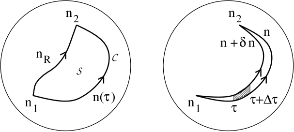
FIG. 9.: The kinetic term in the spin action, and its variation

it is obviously nonsingular.

The actual evaluation of ${\cal A}$ for any given closed path is often more simply done by using Stokes’s theorem to transform it to a line integral. Using notation borrowed from electromagnetism, let us write $d\Omega={\bf B}\cdot{\bf{\hat{n}}}ds$, where ${\bf B}({\bf{\hat{n}}})={\bf{\hat{n}}}$, and $ds$ is an area element. The line integral is $\int{\bf A}\cdot d{\bf{\hat{n}}}$, with ${\bf B}=\nabla\times{\bf A}$. Since ${\bf B}={\bf{\hat{n}}}$, it is the magnetic field of a monopole. It is known that if we try and represent a monopole field in terms of a vector potential ${\bf A}$, then ${\bf A}$ must have a singularity somewhere. If this singularity is concentrated into a Dirac string at the south pole, we can write

$${\cal A}[{\bf{\hat{n}}}(\tau)]=\oint_{{\cal C}}\bigl{[}1-\cos\theta(\phi)\bigr{]}\,d\phi,$$ (36)

where the curve ${\cal C}$ is regarded as being parametrized by $\phi$. This formula is correct as long as ${\cal C}$ does not pass through the south pole, and provided one increments or decrements $\phi$ by $2\pi$ every time one crosses the date line.

Let us now obtain the classical equations of motion by varying the action. Consider the kinetic term first. Suppose we vary the path ${\bf{\hat{n}}}(\tau)$. The variation $\delta{\cal A}$ is given by the area of the thin sliver on the sphere enclosed between the curves ${\bf{\hat{n}}}(\tau)$ to ${\bf{\hat{n}}}(\tau)+\delta{\bf{\hat{n}}}(\tau)$ (Fig. 9). The part of this area due to the segments between $\tau$ and $\tau+\delta\tau$ is given by

$$\Delta(\delta{\cal A}) = \Bigl{[}\delta{\bf{\hat{n}}}(\tau)\times[{\bf{\hat{n}}}(\tau+\Delta\tau)-{\bf{\hat{n}}}(\tau)]\Bigr{]}\cdot{\bf{\hat{n}}}(\tau)$$ (37)

$$= \left(\delta{\bf{\hat{n}}}(\tau)\times{d{\bf{\hat{n}}}\over d\tau}\right)\cdot{\bf{\hat{n}}}(\tau)\Delta\tau.$$ (38)

Adding up the contributions from all the segments, we find the total change

$$\delta{\cal A}=\int\delta{\bf{\hat{n}}}(\tau)\cdot\left({d{\bf{\hat{n}}}\over d\tau}\times{\bf{\hat{n}}}(\tau)\right)\,d\tau.$$ (39)

The variation of the second term in Eq. (34) is

$$\int\delta{\bf{\hat{n}}}(\tau)\cdot{\partial E_{\rm cl}\over\partial{\bf{\hat{n}}}}d\tau.$$ (40)

Thus the variation of $S$ can be written as an integral of the form $\int\delta{\bf{\hat{n}}}(\tau)\cdot X$ where $X$ is something depending on ${\bf{\hat{n}}}$ and $E_{\rm cl}$. The condition for $\delta S$ to vanish is thus $X=0$, or

$$iJ{d{\bf{\hat{n}}}\over d\tau}\times{\bf{\hat{n}}}(\tau)+{\partial E_{\rm cl}\over\partial{\bf{\hat{n}}}}=0.$$ (41)

Taking the cross product of this equation with ${\bf{\hat{n}}}$, and making use of the fact that ${\bf{\hat{n}}}\cdot(d{\bf{\hat{n}}}/d\tau)=0$, we get

$$iJ{d{\bf{\hat{n}}}\over d\tau}=-\left({\bf{\hat{n}}}\times{\partial E_{\rm cl}\over\partial{\bf{\hat{n}}}}\right).$$ (42)

This equation is exactly what we would get from Eq. (5) with ${\bf J}=J{\bf{\hat{n}}}$ and the Wick rotation $t\to-i\tau$. In other words, it is the imaginary time equation for Larmor precession in the effective magnetic field $\partial E_{\rm cl}/\partial{\bf{\hat{n}}}$. (It is also called the Landau-Lishitz equation in magnetism.)

One consequence of Eq. (42) is that $E_{\rm cl}$ is conserved along the classical path. For,

$${dE_{\rm cl}\over d\tau} = {\partial E_{\rm cl}\over\partial{\bf{\hat{n}}}}\cdot{d{\bf{\hat{n}}}\over d\tau}$$ (43)

$$= {i\over J}{\partial E_{\rm cl}\over\partial{\bf{\hat{n}}}}\cdot\left({\bf{\hat{n}}}\times{\partial E_{\rm cl}\over\partial{\bf{\hat{n}}}}\right)$$ (44)

$$= 0.$$ (45)

[Another way to see this is that if Eq. (42) is written in terms of spherical polar coordinates, it will be seen to have a Hamiltonian structure with $\phi$ and $J\cos\theta$ as canonically conjugate variables, and $E_{\rm cl}$ as the Hamiltonian.]

C How to calculate the propagator: instantons

The path integral (24) is not easy to evaluate. In the $T\to\infty$ limit, however, we can use the approximation of steepest descents. The dominant paths, known as instantons, are just those that minimize the action, i.e. they are solutions to the classical equations of motion. The simplest such paths consist of a single transit fro ${\bf{\hat{n}}}_{1}$ to ${\bf{\hat{n}}}_{2}$. If the scale over which $E_{\rm cl}$ varies is $V$, then it follows from Eq. (42) that the time scale for this transit is $\tau_{0}\sim J/V$. For the toy Hamiltonian (2), e.g., this time scale is $J^{-1}(k_{1}k_{2})^{-1/2}$. Since $T\to\infty$, it follows that the spin spends most of its time near the end points ${\bf{\hat{n}}}_{1,2}$, and the actual transit takes place in a very short time interval. (Hence the name instanton.) Further, since the equation of motion is autonomous, i.e., does not depend on $\tau$ explicitly, in the $T\to\infty$ limit, it is clear that a translation of the center of the instanton yields an equally good classical path. Once this is realized, it is not difficult to see that one can have multi-instanton solutions, in which the path goes between ${\bf{\hat{n}}}_{1}$ and ${\bf{\hat{n}}}_{2}$ several times, with the centers of the instantons being widely separated on the time scale $\tau_{0}$. When all the contributions to $U_{21}$ are evaluated in this way, one finds that the $n$-instanton terms give a contribution proportional to $T^{n}$, and the full series is that of a $\sinh$ [46]. The $\Delta$ which is obtained in this way can be written as

$$\Delta=D\exp(-S_{\rm inst}),$$ (46)

where $S_{\rm inst}$ is the action for a single instanton path, and $D$ is a prefactor arising from doing the path-integral over small fluctuations about the instanton trajectory. If more than one instanton exists, we must add together the corresponding contributions from all of them.

It is important to note that since $E_{\rm cl}$ is conserved along the instantons, and since ${\bf{\hat{n}}}_{1}$ and ${\bf{\hat{n}}}_{2}$ are minima of $E_{\rm cl}$, there can not be any real path ${\bf{\hat{n}}}(\tau)$ conecting them. The only solution is to allow ${\bf{\hat{n}}}$ to become complex. Correspondingly, the area ${\cal A}$ must be defined on the complexified unit sphere. We can take $E_{\rm cl}$ to be zero for an instanton by adjusting the zero of energy, so the action is just $iJ{\cal A}$. The problem is thus reduced to finding the instantons and the corresponding area. This is extremely simple, however. Since we can write ${\cal A}[{\bf{\hat{n}}}(\tau)]$ as the line integral (36), we do not need to find the actual time dependence of the instanton path, and it suffices to find the orbit on the unit sphere, i.e., $\theta$ in terms of $\phi$, which can be done from energy conservation alone.

D Application to Fe₈

Let us illustrate this procedure for Fe₈, with the Hamiltonian ${\cal H}_{0}$ for the case where ${\bf H}\|{\bf{\hat{x}}}$. If we choose the polar axis to be ${\bf{\hat{x}}}$ (not ${\bf{\hat{z}}}$), and measure the azimuthal angle in the yz plane from ${\bf{\hat{y}}}$, then we can write

$$E_{\rm cl}(\theta,\phi)=k_{1}J^{2}(\cos\theta-\cos\theta_{0})^{2}+k_{2}J^{2}\sin^{2}\theta\sin^{2}\phi.$$ (47)

We have defined $\cos\theta_{0}=H/H_{c}$, with $H_{c}=2k_{1}J/g\mu_{B}$, and added a constant to $E_{\rm cl}$ so that it vanishes at the minima $(\theta,\phi)=(\theta_{0},0)$ and $(\theta_{0},\pi)$. Thus, along the instanton, $E_{\rm cl}=0$. Writing $\cos\theta_{0}=u_{0}$, the solution of this equation gives

$$\cos\theta={u_{0}+i\lambda^{1/2}\sin\phi(1-u_{0}^{2}-\lambda\sin^{2}\phi)^{1/2}\over 1-\lambda\sin^{2}\phi}.$$ (48)

It is clear from symmetry that there are two instanton paths, which wind about ${\bf{\hat{x}}}$ in opposite directions (see Fig. 1 again). We take $\phi(-\infty)=0$ and $\phi(\infty)=\pm\pi$ for these paths. If we denote the two paths by A and B, then the real parts of their actions ($=iJ{\cal A}$) are equal:

$$S_{R} = {\rm Re}S_{A,B}=J\lambda^{1/2}\int_{0}^{\pm\pi}{\sin\phi(1-u_{0}^{2}-\lambda\sin^{2}\phi)^{1/2}\over 1-\lambda\sin^{2}\phi}d\phi,$$ (49)

$$= J\left[\ln\left({\sqrt{1-u_{0}^{2}}+\sqrt{\lambda}\over\sqrt{1-u_{0}^{2}}-\sqrt{\lambda}}\right)-{u_{0}\over\sqrt{1-\lambda}}\ln\left({\sqrt{(1-u_{0}^{2})(1-\lambda)}+u_{0}\sqrt{\lambda}\over\sqrt{(1-u_{0}^{2})(1-\lambda)}-u_{0}\sqrt{\lambda}}\right)\right].$$ (50)

The imaginary parts, on the other hand are necessarily unequal, since by the interpretation of ${\cal A}$ as an area,

$$S_{B}-S_{A}=iJ\times\Omega,$$ (51)

where $\Omega$ [See Eq. (35)] is the area enclosed between A and B. From Eq. (36) we obtain,

$$\Omega=\int_{-\pi}^{\pi}\left(1-{u_{0}\over 1-\lambda\sin^{2}\phi}\right)d\phi=2\pi\left(1-{u_{0}\over\sqrt{1-\lambda}}\right).$$ (52)

Since $\Delta\propto\cos(J\Omega/2)$, we conclude that it vanishes whenever

$${H\over H_{c}}={\sqrt{1-\lambda}\over J}\Bigl{[}J-n-\textstyle{1\over 2}\Bigr{]},$$ (53)

in exact accord with Eq. (21) (put $\ell=\ell^{\prime}=0$). Although the precise location of the quenching points will change if the Hamiltonian is varied, the effect is clearly general.

E Tunneling prefactors

The above discussion does not explain how the prefactor $D$ is to be calculated. In fact, this calculation is somewhat more subtle for spin than it is for massive particles. If one evaluates the Gaussian fluctuations that yield the prefactor naively, directly following the massive particle case, the result is then not asymptotically correct as $J\to\infty$ [50]. This point is perhaps not of great concern for numerical estimates of tunneling rates in a genuine physical setting, but it is nevertheless an annoying gap in the formalism. Although there do exist other path integral aproaches which find the splitting correctly [51, 52], the calculations are very intricate, and the simplicity seen in the massive particle case is lost.

To describe these subtleties, let us first consider the analog of the propagator (24) for a massive non relativistic particle with a geometrical position coordinate $q$. This is just the amplitude to go from a state $|q_{i}\rangle$ at $t=t_{i}$ to a state $|q_{f}\rangle$ at $t=t_{f}$. Further, it is useful to let $q_{i}$ and $q_{f}$ be completely general, i.e., not necessarily minima of the potential energy, and also to consider the propagator for real time. If we write this amplitude as a Feynman path integral [47], in the semi-classical limit it is again dominated by the classical paths, for which the action $S_{\rm cl}$ is least. Paths far away from the classical one have phases that vary extremely rapidly under small changes of the path, and thus these paths end up canceling each other. A great deal of quantum mechanics can be understood just by stringing a phase factor $\exp(iS_{\rm cl}/\hbar)$ on the classical trajectories. If one wants to get the actual magnitudes of transition amplitudes, however, one must go a little further, and evaluate the integral over the small fluctuations about the classical path. This gives rise to the so-called fluctuation or van Vleck determinant, which is a prefactor multiplying the phase factor $\exp(iS_{\rm cl}/\hbar)$, c.f. Ref.[53]. (The phase and prefactor correspond approximately to the eikonal and transport equations in the standard WKB method.)

For spin path integrals, the fluctuation determinant is more difficult, because in contrast to the particle states for which $\langle q|q^{\prime}\rangle=0$ if $q\neq q^{\prime}$, spin coherent states are not orthogonal: $\langle{\bf{\hat{n}}}|{\bf{\hat{n}}}^{\prime}\rangle\neq 0$ in general even if ${\bf{\hat{n}}}\neq{\bf{\hat{n}}}^{\prime}$. At first sight, it seems that one should include discontinuous paths among the fluctuations. It turns out however, that this is not so, and by discrete time dissection of the path integral, the analog of the van Vleck determinant can be found provided one pays careful attention to the boundary conditions on the spin path. This has been done by several authors[54, 55, 56, 57], but the results do not seem to be widely known. It seems to this author, that once the van Vleck prefactor is understood, tunneling prefactors should be calculable with the same degree of ease as for massive particles [46], but except for some work in Ref. [56] this does not seem to have been widely appreciated yet.

IV The Discrete Phase Integral Method

A Basic formalism: local Bloch waves

The basic idea of the DPI method is to try and solve Schrödinger’s equation in the $J_{z}$ basis as a recursion relation or difference equation. For constant coefficients, linear difference and differential equations can both be solved in terms of exponentials. For slowly varying coefficients, the WKB approach is a powerful one for differential equations, and many of the ideas used there can be carried over to difference equations. With this in mind, let us suppose $|\psi\rangle$ is an eigenstate of ${\cal H}$ with energy $E$. Then, with $J_{z}|m\rangle=m|m\rangle$, $\langle m|\psi\rangle=C_{m}$, $\langle m|{\cal H}|m\rangle=w_{m}$, and $\langle m|{\cal H}|m^{\prime}\rangle=t_{m,m^{\prime}}$ ($m\neq m^{\prime}$), we have

$$\mathop{{\sum}^{\prime}}_{n}t_{m,n}C_{n}+w_{m}C_{m}=EC_{m},$$ (54)

where the prime on the sum indicates that the term $n=m$ is to be omitted.

We can think of Eq. (54) as a tight binding model for an electron in a one-dimensional lattice with sites labelled by $m$, and slowly varying on-site energies ($w_{m}$), nearest-neighbor ($t_{m,m\pm 1}$) hopping terms, next-nearest-neighbor ($t_{m,m\pm 2}$) hopping terms, and so on. In most interesting problems, hopping to very distant neighbors is negligible, and the recursion relation involves only a handful of terms. Since we can think of dynamics in this model in terms of wavepackets, it is clear that there is a generalization of the usual continuum quasiclassical or phase integral method to the lattice case. This is the DPI method.

More specifically, the DPI method is applicable to a recursion relation such as (54) whenever the $w_{m}$ and $t_{m,m\pm\alpha}$ vary sufficiently slowly with $m$. If these quantities were independent of $m$, the solutions to Eq. (54) would be Bloch waves $C_{m}=\exp(iqm)$, with an energy

$$E=w_{m}+2t_{m,m+1}\cos q+2t_{m,m+2}\cos 2q\equiv E(q),$$ (55)

To save writing, it is sometimes useful to identify $w_{m}\equiv t_{m,m}$, and we shall use the notations $w_{m}$ and $t_{m,m}$ interchangably. If for fixed $\alpha$, the $t_{m,m+\alpha}$ vary slowly with $m$ (where the meaning of this term remains to be made precise), we expect it to be a good approximation to introduce a local Bloch wavevector, $q(m)$, and write $C_{m}$ as an exponential $e^{i\Phi}$, whose phase $\Phi$ accumulates approximately as the integral of $q(m)$ with increasing $m$, in exactly the same way that in the continuum quasiclassical method in one dimension, one writes the wavefunction as $\exp(iS(x)/\hbar)$, and approximates $S(x)$ as the integral of the local momentum $p(x)$.

Previous work with the DPI method [19, 20, 58, 21, 22] has been limited to the case where the recursion relation has only three terms, i.e., only nearest neighbor hopping is present. As discussed by Braun, the DPI approximation has been employed in many problems in quantum mechanics where the Schrödinger equation turns into a three-term recursion relation in a suitable basis. All the types of problems as in the continuum case can then be treated—Bohr-Sommerfeld quantization, barrier penetration, tunneling in symmetric double wells, etc. In addition, one can also use the method to give asymptotic solutions for various recursion relations of mathematical physics, such as those for the Mathieu equation, Hermite polynomials, Bessel functions, and so on. The general procedures are well known and simple to state. For any $E$, one solves the Hamilton-Jacobi and transport equations to obtain $q(m)$ and $v(m)$, and writes $C_{m}$ as a linear combinations of the independent solutions that result. The interesting features all arise from a single fact — that the DPI approximation breaks down at the so-called turning points. These are points where $v(m)$ vanishes. One must relate the DPI solutions on opposite sides of the turning point by connection formulas, and the solution of all the various types of problems mentioned above depends on judicious use of these formulas.

In the Fe₈ problem, the recursion relation involves five terms. The diagonal terms ($w_{m}$) arise from the $J_{z}^{2}$ and $J_{z}H_{z}$ parts of ${\cal H}$, the $t_{m,m\pm 1}$ terms from the $J_{x}H_{x}$ part, and the $t_{m,m\pm 2}$ terms from the $J_{x}^{2}$ part. This gives rise to new features over and above the three term case. In particular, we encounter nonclassical turning points, i.e., turning points at $m$ values other than those at the limits of the classically allowed motion. It is these turning points that give rise to oscillatory tunnel splittings, so that this effect is absent in systems described by three-term recursion relations.

The fundamental requirement for a quasiclassical approach to work is that $w_{m}$ and $t_{m,m\pm\alpha}$ ($\alpha=1,2$) vary slowly enough with $m$ that we can find smooth continuum approximants $w(m)$ and $t_{\alpha}(m)$, such that whenever $m$ is an eigenvalue of $J_{z}$, we have

$$w(m) = w_{m},$$ (56)

$$t_{\alpha}(m) = (t_{m,m+\alpha}+t_{m,m-\alpha})/2,\quad\alpha=1,2.$$ (57)

We further demand that

$${dw\over dm}=O\left({w(m)\over J}\right),\quad{dt_{\alpha}\over dm}=O\left({t_{\alpha}(m)\over J}\right),$$ (58)

with $m/J$ being treated as quantity of order 1. Problems for which these conditions cannot be met are not amenable to the DPI method. It is not difficult to see that for Eqs. (7) and (8), these conditions will hold in the semiclassical limit $J\gg 1$.

Given these conditions, the basic approximation, which readers will recognize from the continuum case, is to write the wavefunction as a linear combination of the quasiclassical forms

$$C_{m}\sim{1\over\sqrt{v(m)}}\exp\left(i\int^{m}q(m^{\prime})dm^{\prime}\right),$$ (59)

where $q(m)$ and $v(m)$ obey the equations

$$E = w(m)+2t_{1}(m)\cos q+2t_{2}(m)\cos(2q)\equiv{{\cal H}_{\rm sc}}(q,m),$$ (60)

$$v(m) = \partial{{\cal H}_{\rm sc}}/\partial q=-2\sin q(m)\big{(}t_{1}(m)+4t_{2}(m)\cos q(m)\bigr{)}.$$ (61)

Equations (60) and (61) are the lattice analogs of the eikonal and transport equations. Equation (59) represents the first two terms in an expansion of $\log C_{m}$ in powers of $1/J$.

B Turning points and connection formulas

The basic DPI approximation fails whenever $v(m)=\partial{{\cal H}_{\rm sc}}(q,m)/\partial q=0$, because then it diverges. We shall call all such points turning points in analogy with the continuum case. In contrast to that case, however, we will find that turning points are not just the limits of the classical motion for a given energy, once the notion of the classically accessible region is suitably understood.

Since we must also obey the eikonal equation (60) in addition to the condition $v(m)=0$, at a turning point both $m$ and $q$ are determined if $E$ is given. Setting $v=0$ in Eq. (61), we see that we must have either $q=0$, or $q=\pi$, or $q=q_{*}(m)$, where

$$\cos q_{*}(m)=-t_{1}(m)/4t_{2}(m).$$ (62)

Substituting these values of $q$ in the eikonal equation, we see that a turning point arises whenever

$$E=U_{0}(m),\ U_{\pi}(m),\ {\rm or}\ U_{*}(m),$$ (63)

where,

$$U_{0}(m) = {{\cal H}_{\rm sc}}(0,m)=w(m)+2t_{1}(m)+2t_{2}(m),$$ (64)

$$U_{\pi}(m) = {{\cal H}_{\rm sc}}(\pi,m)=w(m)-2t_{1}(m)+2t_{2}(m),$$ (65)

$$U_{*}(m) = {{\cal H}_{\rm sc}}(q_{*},m)=w(m)-2t_{2}(m)-{t_{1}^{2}(m)\over 4t_{2}(m)}.$$ (66)

Note that $q_{*}(m)$ may be complex for some $m$, but since $\cos q_{*}$ is always real, $U_{*}$ is real for all $m$. We shall refer to these three energy curves as critical curves. We shall see that they collectively play the same role as the potential energy in the continuum quasiclassical method.

To better understand the turning points, let us assume that $t_{1}<0$, and $t_{2}>0$. [This is the case for the Hamiltonian (7). We can always arrange for $t_{1}$ to be negative by means of the gauge transformation $C_{m}\to(-1)^{m}C_{m}$. Thus there is only one other case to be considered, namely, $t_{1}<0$, $t_{2}<0$. This is discussed in Ref. [59].] It then follows that $U_{\pi}>U_{0}$, and that

$$U_{0}(m)-U_{*}(m)={1\over 4t_{2}(m)}\bigl{(}t_{1}(m)+4t_{2}(m)\bigr{)}^{2}\geq 0.$$ (67)

Secondly, let us think of ${{\cal H}_{\rm sc}}(q,m)$ for fixed $m$ as an energy band curve. Then $U_{\pi}$ is always the upper band edge, while the lower band edge is either $U_{0}$ or $U_{*}$ according as whether $-t_{1}/4t_{2}$ is greater than or lesser than 1. To deal with this possibility, it pays to introduce a dual labeling scheme for all three curves $U_{0}$, $U_{\pi}$, and $U_{*}$. We write $U_{\pi}(m)\equiv U_{+}(m)$, and

$$U_{0}(m)=U_{i}(m),\ U_{*}(m)=U_{-}(m),\quad{\rm if}\ q_{*}\in(0,\pi),$$ (68)

$$U_{0}(m)=U_{-}(m),\ U_{*}(m)=U_{f}(m),\quad{\rm if}\ q_{*}\not\in(0,\pi).$$ (69)

The subscripts $+$ and $-$ denote upper and lower band edges, while the subscripts i and f denote internal and forbidden respectively, since in the first case above, $U_{0}$ lies inside the

FIG. 10.: Critical energy curves for the Fe₈ Hamiltonian when ${\bf H}\|{\bf{\hat{x}}}$, showing the dual labeling scheme. In the right hand figure, the region near the left minimum of $U_{0}$ is magnified, showing the two turning points $-m_{t}$ and $-m_{1}$.

energy band, while in the second case, $U_{*}$ lies outside. As examples of these curves for a symmetric recursion relation, we show those for Fe₈ in Fig. 10, along with a magnified view of the lower left hand portion.

Turning points where $E=U_{+}$, or $E=U_{-}$ when $U_{-}=U_{0}$, are analogous to those encountered in the continuum quasiclassical method, since the energy lies at a limit of the classically allowed range for the value of $m$ in question. Points where $E=U_{-}$ when $U_{-}=U_{*}$ are physically analogous, but mathematically different since the value of $q_{c}$ is neither $0$ nor $\pi$. Points where $E=U_{i}$ (see the energy $E_{1}$ in Fig. 10, e.g.) are novel in that the energy is inside the classically allowed range for $m_{c}$, but the mathematical form of the connection formulas is identical to the case $E=U_{-}=U_{0}$ since $q_{c}=0$. Most interesting are the turning points with $E=U_{f}$ (the point $m=-m_{1}$ in Fig. 10, for instance), since now the energy is outside the allowed range for $m=m_{c}$, and the value of $q_{c}$ is therefore necessarily complex. These points lie “under the barrier” and turn out to be the ones of importance for understanding oscillatory tunnel splittings. The derivation of connection formulas at these turning points is not particularly difficult, but quite lengthy. In fact, it is quite lengthy to even quote the connection formulas themselves, and we refer readers to Ref. [59] for the details. The key point is that a solution with a purely imaginary $q$ on side of the turning point, representing, let us say a solution that decays with growing $m$, turns on the other side into a solution with a complex $q$ with a nonzero real part, representing a solution that decays with an oscillating envelope as $m$ increases. These kinds of wavefunctions can simply never arise in conventional one-dimensional continuum problems.

From this point on, the exercise of calculating tunnel splittings is exactly as in the continuum case. One demands that the wavefunctions decay as $m\to\pm\infty$ and applies connection formulas at the turning points to continue the wavefunction into the interior. Finally near $m=0$, one demands that the wavefunctions so found from the two sides should agree. This gives the eigenvalue condition. The one new complication (besides the new turning points) is that at each $m$, there are four solutions to the Hamilton-Jacobi equation instead of two in the continuum case. As $m\to-\infty$, all four $q$’s are pure imaginary, but of these only the two which are negative imaginary can be kept. Thus at every point $m$, one must keep track of two DPI solutions. An exception to this arises in the case of symmetric double wells (${\bf H}\|{\bf{\hat{x}}}$), where Herring’s formula [60] simplifies matters, and one can work purely with a wavefunction that decays away from one of the wells in both directions. This formula is sufficiently important to be worth discussing separately. We do this in the next subsection, present results that follow from its application in the succeeding subsection, and for the asymmetric case in the one following that.

C The symmetric case; Herring’s formula

It is useful to recall a basic formula for tunnel splittings in symmetric potentials [$V(-x)=V(x)$] for massive particles [61]. Let the minima be at $x=\pm a$, and let $\psi_{0}(x)$ be a wavefunction localized entirely in the right hand well, with an energy $E_{0}$. This wavefunction obviously does not obey Schrodinger’s equation near the left hand well, and we could imagine modifying the potential suitably in that region so that the wavefunction continues to decay wtih decreasing $x$ even in the vicinity of the left well. Since we will never need $\psi_{0}(-a)$, the precise way in which this is done is not important.

If $E_{0}$ is well below the barrier, then we expect there to be two states $\psi_{s}$ and $\psi_{a}$, with energies $E_{1}$ and $E_{2}$, both very close to $E_{0}$, and with wavefunctions that are very accurately given by

$$\psi_{s,a}={1\over\sqrt{2}}\bigl{[}\psi_{0}(x)\pm\psi_{0}(-x)\bigr{]}.$$ (70)

The product $\psi_{0}(x)\psi_{0}(-x)$ is everywhere exponentially small, and so therefore, if the wavefunction $\psi_{0}(x)$ is normalized, so are $\psi_{s,a}$. For the same reason,

$$\int_{0}^{\infty}\psi_{0}(x)\psi_{a}(x)\,dx={1\over\sqrt{2}}.$$ (71)

The differential equations obeyed by $\psi_{0}$ and $\psi_{a}$ in the region $x>0$ are

$$-(\hbar^{2}/2m)\psi^{\prime\prime}_{0}(x)+V(x)\psi_{0}(x) = E_{0}\psi_{0}(x),$$ (72)

$$-(\hbar^{2}/2m)\psi^{\prime\prime}_{a}(x)+V(x)\psi_{a}(x) = E_{2}\psi_{a}(x).$$ (73)

We multiply the first equation by $\psi_{a}$, the second by $\psi_{0}$, subtract, and integrate from $0$ to $\infty$. This yields

$$E_{2}-E_{0} = \sqrt{2}{\hbar^{2}\over 2m}\int_{0}^{\infty}(\psi_{a}\psi_{0}^{\prime\prime}-\psi_{0}\psi_{a}^{\prime\prime})dx$$ (74)

$$= \sqrt{2}{\hbar^{2}\over 2m}[\psi_{a}\psi_{0}^{\prime}-\psi_{0}\psi_{a}^{\prime}]_{0}^{\infty}$$ (75)

$$= {\hbar^{2}\over m}\psi_{0}(0)\psi^{\prime}_{0}(0),$$ (76)

where we have used the facts that $\psi_{0,a}(\infty)=0$, $\psi_{a}(0)=0$, and $\psi^{\prime}_{a}(0)={\sqrt{2}}\psi^{\prime}_{0}(0)$. A similar calculation yields $E_{1}-E_{0}=-(E_{2}-E_{0})$, so that the energy splitting, $\Delta$ is given by

$$\Delta={2\hbar^{2}\over m}\psi_{0}(0)\psi^{\prime}_{0}(0).$$ (77)

This is Herring’s formula. It has a nice and physically appealing interpretation in terms of the probability current at $x=0$.

If we now use the WKB method to find $\psi_{0}(0)$ and $\psi^{\prime}_{0}(0)$, keeping in mind the normalization, for the $n$th pair of levels, we get

$$\Delta_{n}=g_{n}{\hbar\omega\over\pi}\exp\left[-\int_{-a^{\prime}_{n}}^{a^{\prime}_{n}}{|p|\over\hbar}dx\right].$$ (78)

Here, $\omega$ is the small oscillation frequency in the well, $[V^{\prime\prime}(a)/m]^{1/2}$, $\pm a^{\prime}_{n}$ are the classical turning points for the $n$th energy level pair with the mean value $E_{0}\approx(n+{1\over 2})\hbar\omega$, and

$$g_{n}={\sqrt{2\pi}\over n!}\left(n+\textstyle{1\over 2}\right)^{n+{1\over 2}}e^{-(n+{1\over 2})},$$ (79)

Note that if $g_{n}$ were unity, we would have the formula of Ref. [61]. The corrections are small: $g_{0}=(\pi/e)^{1/2}\approx 1.075$, $g_{1}\approx 1.028$, $g_{2}\approx 1.017$, and so on. Stirling’s formula for $n!$ shows that $g_{n}\to 1$ as $n\to\infty$. These corrections are well known to many workers, but not known to many others, and they arise from the fact that as $n$ becomes smaller, the use of a linear turning point formula at the turning point is increasingly inaccurate. The correct procedure is to use quadratic turning point formulas [53]. A pedagogical discussion of this matter may be found in Ref. [62].

One can repeat the above argument for the discrete case making the obvious modifications as needed. The analogue of Eq. (77), Herring’s formula, is

$$\Delta=\cases{2\left[t_{0,1}C_{0}(C_{1}-C_{-1})+t_{0,2}C_{0}(C_{2}-C_{-2})+t_{-1,1}(C_{1}^{2}-C_{-1}^{2})\right],&\\ integer$J$,\cr 2\ t_{-{1\over 2},{1\over 2}}\Bigl{(}C^{2}_{{1\over 2}}-C^{2}_{-{1\over 2}}\Bigr{)}+4\ t_{-{3\over 2},{1\over 2}}\left(C_{{1\over 2}}C_{{3\over 2}}-C_{-{1\over 2}}C_{-{3\over 2}}\right),&half-integer $J$.\cr}$$ (80)

When it is combined with the DPI approximation, one obtains for both integer and half-integer $J$ [27],

$$\Delta={\omega_{0}g_{n}\over 2\pi}\left[\exp\left(i\int_{-m_{t}}^{m_{t}}q(m^{\prime})dm^{\prime}\right)+\ {\rm c.c.}\right].$$ (81)

The similarity to the continuous case is striking. The only point worth remarking is the possibility of having the Bloch vector $q(m)$ be complex in part or all of the tunneling region. In Eq. (81), we have written the formula for the Fe₈ problem, where there are two $q$’s with positive imaginary parts and equal and opposite real parts in the tunneling region.

It may be useful at this point to make a general remark about how tunneling prefactors are obtained in the DPI method. Equations (78) and (81) contain these prefactors naturally, and it is apparent that they arise as a consequence of the $1/\sqrt{v(m)}$ normalization in the general DPI form and the connection formulas at turning points. Provided one can solve the transport equation and apply the connection formulas correctly, these factors are relatively easy to obtain. (We shall see that this continues to be true in the asymmetric case.) Historically, however, one error which has been made is to use linear turning point formulas all throughout, as in Ref. [61]. As already mentioned, this leads one to miss the curvature factors $g_{n}$. This error is widely repeated, perhaps because of the reputation of this text, and perhaps because it is numerically insignificant. From a logical point of view, however, there is no reason not to incorporate the curvature corrections, and they must be kept if one wants an answer for the tunneling amplitude itself (and not just its logarithm) that is properly asymptotic to the true answer as $\hbar\to 0$, or as $J\to\infty$.

D Results for Fe₈ in symmetric case [26]

To apply the general results to Fe₈, we need the explicit forms for $w(m)$, and $t_{\alpha}(m)$. It is convenient to measure energies (including $\omega_{0}$) in units of $k_{1}\bar{J}^{2}$, and introduce the scaled variable $\mu=m/\bar{J}$, where

$$\bar{J}=J+\textstyle{1\over 2}.$$ (82)

In these variables, when ${\bf H}\|{\bf{\hat{x}}}$, we get (with $h_{x}=JH_{x}/\bar{J}H_{c}$)

$$w(m) = (1+\lambda)(1-\mu^{2})/2,$$ (83)

$$t_{1}(m) = -h_{x}(1-\mu^{2})^{1/2},$$ (84)

$$t_{2}(m) = (1-\lambda)(1-\mu^{2})/4.$$ (85)

The actual evaluation of the integrals is mostly a matter of careful but straightforward analysis, and the final answer for the splitting can be written as

$$\Delta_{n}={1\over n!}\sqrt{8\over\pi}\omega_{0}F^{n+{1\over 2}}e^{-\Gamma_{0}}\cos\Lambda_{n},$$ (86)

where,

$$\omega_{0} = 2J[k_{1}k_{2}(1-h_{x0}^{2})]^{1/2},$$ (87)

$$F = 8J{\lambda^{1/2}(1-h_{x}^{2})^{3/2}\over 1-\lambda-h_{x}^{2}},$$ (88)

$$\Gamma_{0} = \bar{J}\left[\ln\left({\sqrt{1-u_{0}^{2}}+\sqrt{\lambda}\over\sqrt{1-u_{0}^{2}}-\sqrt{\lambda}}\right)-{h_{x}\over\sqrt{1-\lambda}}\ln\left({\sqrt{(1-u_{0}^{2})(1-\lambda)}+h_{x}\sqrt{\lambda}\over\sqrt{(1-u_{0}^{2})(1-\lambda)}-h_{x}\sqrt{\lambda}}\right)\right],$$ (89)

$$\Lambda_{n} = {{\rm max}}\left\{0,\ \pi J\left(1-{H_{x}\over\sqrt{1-\lambda}H_{c}}\right)-n\pi\right\}.$$ (90)

In Eqs. (87–90), $\lambda=k_{2}/k_{1}$, and

$$h_{x}={JH_{x}\over\bar{J}H_{c}},\quad h_{x0}={H_{x}\over H_{c}}.$$ (91)

Recall that $H_{c}=2k_{1}J/g\mu_{B}$.

It is an immediate consequence of these results that $\Delta_{n}$ vanishes when

$${H_{x}\over H_{c}}={\sqrt{1-\lambda}\over J}\left[J-\ell-{1\over 2}\right],$$ (92)

with $\ell=n$, $n+1$, $\ldots$, $2J-n-1$. These are precisely the results quoted in Sec. II.

E Results for Fe₈ in asymmetric case [27]

When ${\bf H}$ has components both along ${\bf{\hat{x}}}$ and ${\bf{\hat{z}}}$, the critical curves are no longer symmetric (Fig. 11), and the problem cannot be reduced to just quoting a splitting. Suppose we consider an energy $E$, as drawn in Fig. 11, and suppose that it leads to turning points at $m^{\prime}_{a}$, $m^{\prime}_{b}$, $m^{\prime}_{c}$ on the left hand side, and $m^{\prime\prime}_{c}<m^{\prime\prime}_{b}<m^{\prime\prime}_{a}$ on the right. (We denote quantities pertaining to the left hand solution or the left hand side of the well by either a single prime or a suffix

FIG. 11.: Critical energy curves for the Fe₈ Hamiltonian when ${\bf H}$ has both $x$ and $z$ components. In the right hand figure, the region near the left minimum of $U_{0}$ is magnified, showing the various turning points.

$-$, and corresponding right-hand-well quantities by a double prime or a $+$ suffix.) A wavefunction $C^{\prime}_{m}$ which decays as $m\to-\infty$ will possess the following additional characteristics. It will either oscillate or continue to have the same exponential character in the classically allowed region $m^{\prime}_{a}<m<m^{\prime}_{b}$. In the region just to the right of $m^{\prime}_{b}$ it will consist of a decaying part and a growing part. The new feature will be encountered at $m^{\prime}_{c}$ where $E=U_{*}$. For $m>m^{\prime}_{c}$, both the growing and decaying parts will acquire oscillatory envelopes. Similar remarks apply to the right side wavefunction $C^{\prime\prime}_{m}$. The eigenvalue condition will be obtained by matching the wavefunction in the central region $m^{\prime}_{c}\ll m\ll m^{\prime\prime}_{c}$.

Let us now denote the left well minimum by $m_{0-}$, the small oscillation frequency in that well by $\omega_{0-}$, and the value of $U_{0}(m_{0-})$ by $E_{-}$. We write

$$E=E_{-}+(\nu^{\prime}+\textstyle{1\over 2})\omega_{0-}.$$ (93)

In the same way we define analogous quantities for the right hand well. We expect that tunneling will be significant only when the energy $E$ is such that it matches a level in both wells, say, level numbers $\ell^{\prime}$ and $\ell^{\prime\prime}$, where $\ell=0$ is the ground level. Since the problem is harmonic near the two potential wells, we can write the energy levels using a harmonic oscillator formula, and with this in mind, we define an offset $\epsilon^{\prime}$,

$$\nu^{\prime}=\ell^{\prime}+{\epsilon^{\prime}\over\omega_{0-}},$$ (94)

where $\ell^{\prime}$ is a positive integer, and $\epsilon^{\prime}$ lies in the interval $(-1/2,1/2)\omega_{0-}$. $\epsilon^{\prime\prime}$ is similarly defined. Our remarks above mean that mixing between the two wells will be significant only when $\epsilon^{\prime}$ and $\epsilon^{\prime\prime}$ are both small. This is indeed the case, and the matching or eigenvalue condition turns out to be

$$\epsilon^{\prime}\epsilon^{\prime\prime}={1\over 4}[\Delta({\ell^{\prime},\ell^{\prime\prime}})]^{2},$$ (95)

where $\Delta({\ell^{\prime},\ell^{\prime\prime}})$ is an exponentially small tunneling amplitude that we shall give shortly. The essential point emerges if we define

$$\epsilon = \textstyle{1\over 2}(\epsilon^{\prime}+\epsilon^{\prime\prime})=E-{1\over 2}\left(E_{-}+E_{+}+(\ell^{\prime}+\textstyle{1\over 2})\omega_{0-}+(\ell^{\prime\prime}+\textstyle{1\over 2})\omega_{0+}\right),$$ (96)

$$\delta = \epsilon^{\prime\prime}-\epsilon^{\prime}=\left(E_{-}-E_{+}+(\ell^{\prime}+\textstyle{1\over 2})\omega_{0-}-(\ell^{\prime\prime}+\textstyle{1\over 2})\omega_{0+}\right).$$ (97)

Then, the eigenvalue condition Eq. (95) can be rewritten as

$$\epsilon=\pm\textstyle{1\over 2}[\delta^{2}+\Delta^{2}(\ell^{\prime},\ell^{\prime\prime})]^{1/2}.$$ (98)

These are of course, the eigenvalues of the two-level-system Hamiltonian

$${\cal H}_{\rm TLS}={1\over 2}\left(\begin{array}[]{cc}\delta&\Delta({\ell^{\prime},\ell^{\prime\prime}})\\ \Delta({\ell^{\prime},\ell^{\prime\prime}})&-\delta\end{array}\right),$$ (99)

exactly as we should expect. The quantity $\epsilon$ is the energy measured from a convenient reference point, while $\delta$, which depends on the fields $H_{x}$, $H_{z}$, and the quantum numbers $\ell^{\prime}$ and $\ell^{\prime\prime}$ of the states whose mixing is being examined, is the bias or offset between these energy levels in the absence of tunneling. Equation (100) below gives the tunneling amplitude between these levels when the bias is small, i.e., when the two levels are in approximate degeneracy. Note that although this amplitude is defined even for relatively large biases—biases comparable to the intrawell spacings $\omega_{0\pm}$—and indeed is not very sensitive to the value of the bias, the concept of tunneling is physically sensible and useful only when the bias is comparable to or less than the amplitude $\Delta$. If $\delta\gg\Delta$, we get $\epsilon\approx\pm\delta/2$, i.e., $\epsilon^{\prime\prime}\approx\delta$, $\epsilon^{\prime}\approx\Delta^{2}/\delta$, or the other way around. Choosing the first way, we find that $E\approx E_{-}+(\ell^{\prime}+\textstyle{1\over 2})\omega_{0-}$, and a wavefunction essentially given by $(1\quad\Delta^{2}/\delta)^{\rm T}$, i.e., localized in the left well, with negligible mixing with the right well.

It remains to give the expression for $\Delta({\ell^{\prime},\ell^{\prime\prime}})$. This is,

$$\Delta({\ell^{\prime},\ell^{\prime\prime}})={2\over\pi}(g_{\ell^{\prime}}g_{\ell^{\prime\prime}})^{1/2}(\omega_{0-}\omega_{0+})^{1/2}e^{-\Gamma_{G}}\cos\Lambda_{c},$$ (100)

with $\Gamma_{G}$ being the total Gamow factor

$$\Gamma_{G}=\int_{m^{\prime}_{b}}^{m^{\prime\prime}_{b}}|\,{\rm Im}\,q_{1}(m)|\,dm,$$ (101)

and $\Lambda_{c}$ being the phase integral

$$\Lambda_{c}=\int_{m^{\prime}_{c}}^{m^{\prime\prime}_{c}}|\,{\rm Re}\,q(m)|\,dm.$$ (102)

In Eq. (101) the subscript 1 on $q(m)$ means that we are to take that solution of the Hamilton-Jacobi equation which goes to zero at $m^{\prime}_{b}$ and $m^{\prime\prime}_{b}$. In Eq. (102), on the other hand, we can choose any of the four solutions for the wavevector, since they are of the form

$$q(m)=\pm i\kappa(m)\pm\chi(m),$$ (103)

where $\kappa(m)$ and $\chi(m)$ are both real, and the signs can be chosen independently from the two $\pm$ options.

The application of these results to Fe₈ again requires doing a certain number of integrals. The problem of greatest interest is the location of the diabolical points, and for that we need only solve the conditions $\delta=\Delta=0$. The latter condition can only come about when $\Lambda_{c}$ is an odd multiple of $\pi/2$, so in fact we need only give formulas for $\delta$ and $\Lambda_{c}$. We find

$$\delta(h_{z},\ell^{\prime},\ell^{\prime\prime})=4\mu_{0}h_{z}+{2\sqrt{\lambda}\mu_{0}\over\bar{J}}(\ell^{\prime}-\ell^{\prime\prime})-{\sqrt{\lambda}h_{z}\over\bar{J}}(\ell^{\prime}+\ell^{\prime\prime}+1)c_{1}(h_{x})+O(\bar{J}^{-3}),$$ (104)

where

$$c_{1}(h_{x})={1-h_{x}^{2}+\lambda(1+2h_{x}^{2})\over\lambda(1-h_{x}^{2})},$$ (105)

with $h_{z}=JH_{z}/\bar{J}H_{c}$, and $\mu_{0}=(1-h_{x}^{2})^{1/2}$. For $\Lambda_{c}$, we have up to order $J^{0}$,

$$\Lambda_{c}={\pi\over 2}\left[2J-(\ell^{\prime}+\ell^{\prime\prime})-2J{H_{x}\over H_{c}\sqrt{1-\lambda}}\right].$$ (106)

If we ignore the correction $c_{1}(h_{x})$, the conditions $\delta=\Delta=0$ are thus precisely those quoted in Sec. II.

- [1] Electronic address: agarg@nwu.edu
- [2] S. Creagh, Tunneling in Two Dimensions, in Tunneling in Complex Systems, edited by Steven Tomsovic (World Scientific, Singapore, 1978).
- [3] M. Wilkinson, Physica 21 D, 341 (1986).
- [4] I. Ya. Korenbilt and E. F. Shender, Zh. Eksp. Teor. Fiz. 75, 1862 (1978) [Sov. Phys. JETP 48 (1978)].
- [5] E. M. Chudnovsky and L. Gunther, Phys. Rev. Lett. 60, 661 (1988).
- [6] B. Barbara and E. M. Chudnovsky, Phys. Lett. A 145, 205 (1990).
- [7] Leon Gunther and Bernard Barbara, Eds., Quantum Tunneling of Magnetization – QTM ’94, NATO ASI Series E: Applied Sciences, Vol. 301, Proceedings of the NATO Advanced Research Workshop on Quantum Tunneling of Magnetization – QTM ’94, Grenoble and Chichilianne, France, June 27 - July 2, 1994 (Kluwer Academic, Dordecht, 1995).
- [8] M. A. Novak and R. Sessoli, in Ref. [7].
- [9] J. Friedman, M. P. Sarachik, J. Tejada, and R. Ziolo, Phys. Rev. Lett. 76, 3830 (1996).
- [10] L. Thomas et al., Nature 383, 145 (1996).
- [11] J. Villain, F. Hartman-Boutron, R. Sessoli, and A. Rettori, Europhys. Lett. 27, 159 (1994).
- [12] A. Garg, Phys. Rev. Lett. 81, 1513 (1998).
- [13] W. Wernsdorfer and R. Sessoli, Science 284, 133 (1999)
- [14] D. Loss, D. P. DiVincenzo, and G. Grinstein, Phys. Rev. Lett. 69, 3232 (1992).
- [15] J. von Delft and C. L. Henley, Phys. Rev. Lett. 69, 3236 (1992).
- [16] A. Garg, Europhys. Lett. 22, 205 (1993).
- [17] J. R. Klauder, in Path Integrals (Proceedings of the NATO Advanced Summer Institute), edited by G. J. Papadopoulos and J. T. Devreese (Plenum, NY, 1978).
- [18] J. R. Klauder, Phys. Rev. D 19, 2349 (1979).
- [19] R. B. Dingle and J. Morgan, Appl. Sci. Res. 18, 221 (1967); ibid. 18, 238 (1967).
- [20] K. Schulten and R. G. Gordon, J. Math. Phys. 16, 1971 (1975).
- [21] P. A. Braun, Rev. Mod. Phys. 65, 115 (1993).
- [22] J. L. van Hemmen and A. Sütő, (a) Europhys. Lett. 1, 481 (1986); (b) Physica 141B, 37 (1986).
- [23] J. L. van Hemmen and W. F. Wreszinski, Commun. Math. Phys. 119, 213 (1988).
- [24] J. L. van Hemmen and A. Sütő, in Ref. [7].
- [25] A. Garg, Phys. Rev. Lett. 83, 4385 (1999).
- [26] J. Villain and Anna Fort, Euro. Phys. J. B 17, 69 (2000).
- [27] A. Garg, to appear in Phys. Rev. B; cond-mat/0003114.
- [28] A. Garg, to appear in Phys. Rev. B; cond-mat/0003156.
- [29] K. Wieghardt, K. Pohl, I. Jibril, and G. Huttner, Angew. Chem. Int. Ed. Engl. 23, 77 (1984)
- [30] C. Delfs et al., Inorg. Chem. 32, 3099 (1993).
- [31] A. -L. Barra, P. Debrunner, D. Gatteschi, Ch. E. Schultz, and R. Sessoli, Europhys. Lett. 35, 133 (1996).
- [32] C. Sangregorio, T. Ohm, C. Paulsen, R. Sessoli, and D. Gatteschi, Phys. Rev. Lett. 78, 4645 (1997).
- [33] R. Caciuffo, G. Amoretti, A. Murani, R. Sessoli, A. Caneschi, and D. Gatteschi, Phys. Rev. Lett. 81, 4744 (1998).
- [34] T. Ohm, C. Sangregorio, and C. Paulsen, Eur. Phys. J. B 6, 195 (1998).
- [35] L. D. Landau, Phys. Z. Sowjetunion 2, 46 (1932); C. Zener, Proc. Roy. Soc. London A 137, 696 (1932); E. C. G. Stückelberg, Helv. Phys. Acta 5, 369 (1932).
- [36] L. D. Landau and E. M. Lifshitz, Quantum Mechanics 3rd edition, (Pergamon, New York, 1977), Sec. 90.
- [37] W. Wernsdorfer, R. Sessoli, A. Caneschi, D. Gatteschi, and A. Cornia, J. Appl. Phys. 87, 5481 (2000).
- [38] J. von Neumann and E. P. Wigner, Physik. Z. 30, 467 (1929).
- [39] V. I. Arnold, Mathematical Methods of Classical Mechanics (Springer-Verlag, New York, N.Y., 1978). See Appendix 10. More precisely, the theorem is that the codimension of the space of a double degeneracy is 2 or 3, when the dimensionality of the parameter space exceeds 2 for real, or 3 for complex Hamiltonians, respectively. Another lucid and perceptive discussion may be found in C. A. Mead, J. Chem. Phys. 70, 2276 (1979).
- [40] M. V. Berry and M. Wilkinson, Proc. Roy. Soc. Lond. A 392, 15 (1984).
- [41] G. Herzberg and H. C. Longuet-Higgins, Discuss. Faraday Soc. 35, 77 (1963).
- [42] A. Garg, Phys. Rev. B 51, 15161 (1995).
- [43] Ersin Keçecioğlu and A. Garg, to appear in Phys. Rev. B; cond-mat/0003319.
- [44] M. V. Berry, Proc. R. Soc. Lond. A 392, 45 (1984).
- [45] J. S. Langer, Ann. Phys. (N.Y.) 41, 108 (1967).
- [46] S. Coleman, Phys. Rev. D 15, 2929 (1977); Aspects of Symmetry (Cambridge University Press, Cambridge, 1985), Chap. 7.
- [47] R. Shankar, Principles of Quantum Mechanics (Plenum, New York, 1980), Chap. 8.
- [48] F. D. M. Haldane, Phys. Lett. A 93, 464 (1983); Phys. Rev. Lett. 50, 1153 (1983); J. Appl. Phys. 57, 3359 (1985).
- [49] E. Fradkin, Field Theories of Condensed Matter Systems (Addison-Wesley, Redwood City, 1991), Chap. 5.
- [50] A. Garg and G.-H. Kim, Phys. Rev. B 45, 921 (1992).
- [51] M. Enz and R. Schilling, J. Phys. C 19, L711 and 1765 (1986).
- [52] V. I. Belinicher, C. Providencia, and J. da Providencia, J. Phys. A: Math. Gen. 30, 5633 (1997).
- [53] M. V. Berry and K. E. Mount, Rep. Prog. Phys. 35, 315 (1972).
- [54] H. G. Solari, J. Math. Phys. 27, 1097 (1987).
- [55] E. A. Kochetov, J. Math. Phys. 36, 4667 (1995).
- [56] V. R. Vieira and P. D. Sacramento, Nuc. Phys. B 448, 331 (1999).
- [57] M. Stone, K. S. Park, and A. Garg, J. Math. Phys. 41, 8025 (2000).
- [58] P. A. Braun, Teor. Mat. Fizika 37, 355 (1978) [Sov. Phys. Theor. Math. Phys. 37, 1070 (1978)].
- [59] A. Garg, math-ph/0003005.
- [60] Conyers Herring, Rev. Mod. Phys. 34, 631 (1962).
- [61] See Ref. [36], Sec. 50, problem 3.
- [62] A. Garg, Amer. J. Phys. 68, 430 (2000).