Interaction potential between dynamic dipoles: polarized excitons in strong magnetic fields

Abstract

The interaction potential of a two-dimensional system of excitons with spatially separated electron-hole layers is considered in the strong magnetic field limit. The excitons are assumed to have free dynamics in the $x$-$y$ plane, while being constrained or ‘polarized’ in the $z$ direction. The model simulates semiconductor double layer systems under strong magnetic field normal to the layers. The residual interaction between excitons exhibits interesting features, arising from the coupling of the center-of-mass and internal degrees of freedom of the exciton in the magnetic field. This coupling induces a dynamical dipole moment proportional to the center-of-mass magnetic moment of the exciton. We show the explicit dependence of the inter-exciton potential matrix elements, and discuss the underlying physics. The unusual features of the interaction potential would be reflected in the collective response and non-equilibrium properties of such system.

I Introduction

The availability of new materials and interfaces in semiconductors has allowed the exploration of novel electronic systems with fascinating physical behavior. Of particular relevance to the model studied in this paper are the structures achieved by clever use of multi-layer geometries, yielding double quantum wells, and heterojunction interfaces of type II. In those systems, either by the application of external electric fields or by the intrinsic structure potentials, it is possible to achieve separation of electrons and holes into distinct parallel layers, while controlling the in-plane carrier densities.

This situation, of spatially separated electron and hole layers has attracted the attention of several groups, both in theory and experiment. The early proposals of Kogan and Tavger, [1] as well as Lozovik and Yudson, [2] and Shevchenko, [3] were focused on the possible correlations in such systems due to the electron-hole interactions across the layers. More recently, other authors have theoretically explored different features of these systems, from possible vortices, [4] and dark excitonic states due to hidden symmetries, [5] to the various non-trivial thermodynamic phases of these systems. [6] On the experimental side, there has been substantial activity as well. The experiments of Fukuzawa and coworkers gave tantalizing evidence for the anticipated Bose condensation of ‘spatially indirect’ excitons in double quantum wells under strong electric fields. [7] Although later work has shown that the interpretation of those results was not reliable, [8] given the characteristics of the samples used, the concepts of achieving Bose condensation of excitons in quantum wells is sound, experimentally feasible, and currently being pursued in new geometries and systems. [9]

Controlled electron-hole separation in different layers/planes has also been achieved using heterojunctions of type II, such as those formed between InAs and AlSb (or GaSb). In these structures, the band alignments are such that electrons and holes are spatially separated in equilibrium, as the bottom of the conduction band on one side of the heterojunction lies lower than the top of the valence band on the other. Butov et al. [10] have reported photoluminescence experiments in AlAs/GaAs heterojunctions, and their results suggest the appearance of a Bose condensate in at least the high magnetic field regime. Kono et al. have also reported interesting spectroscopic data suggesting an infrared-active state in the InAs/Al_xGa_1-xSb system with unusual properties, reminiscent also of those of a condensate. [11] Although the carriers in these latter systems are not introduced optically (as in the experiments above), the close proximity of carriers across layers, while remaining at relatively low densities, may yield exciton-like bound states of electrons and holes.

Depending on the details of each system, one can identify suitable conditions under which the electron-hole layers would be well described as a collection of polarized exciton-like dipoles. [2] These conditions require the in-plane separation of charge carriers to be much larger than that across the layers (so that the electron-electron or hole-hole distances in each plane are larger than those between electron and hole planes). This in turn yields a system of excitonic dipoles predominantly polarized along the normal to the interface. We present here a study of the interactions between the resulting exciton states, taking into account both the presence of an intense magnetic field, and the internal structure of the electron-hole pair. The presence of the magnetic field introduces a dynamical coupling between the center of mass of the exciton and its relative coordinate, so that the exciton-exciton scattering is a much more complicated event than that occurring between point charges. We discuss here these interactions, the potential characteristics and different scattering events possible.

We should mention that perhaps the closest analog of these polarized interacting excitons is that provided by polar molecules, such as CO or HF. A large number of theoretical and experimental studies of the scattering events between such molecules exists in the literature. [12] Although such systems have permanent dipole moments and live in three dimensions, the most different aspect to the excitons here is the non-trivial coupling of their internal degrees of freedom with the center-of-mass magnetic momentum. This feature adds a very interesting and subtle complication to the excitonic systems studied here.

In fact, we will show that unlike more compact composite objects, or in the polar-molecule analog, the scattering events here can strongly affect the internal state of the participating excitons. In fact, as the in-plane dipole moment of the exciton is proportional to its center-of-mass magnetic momentum, the scattering will in general re-orient the dipole in a well-defined way which depends on the momenta of the participating excitons. The event may also cause transitions to excited internal states of the exciton, just as in the polar molecule analog, although those may be suppressed here by the strong magnetic field. This article studies the details of such momentum exchanges and effective interactions, and provides explicit expressions for the lowest matrix elements. Apart from describing an unusual and interesting situation, these interactions would play a vital role in a description of the collective modes of this interacting boson gas.

It is also interesting to note the similarity of these exciton dipoles with those believed to exist in the quantum Hall regime at half-filling of Landau level. The composite fermions there develop a dipole moment proportional to the momentum, in a similar way to the excitons we describe. Although the underlying physics is quite different, the scattering events of the effective quasi-particles are possibly quite similar. [13] Perhaps some of the intuition developed in our study of excitons would be of some use in better understanding composite fermions in that regime.

In what follows, the specifics of the model are described in section II, including a description of the role of magnetic field in coupling the various degrees of freedom. Section III describes then the potential matrix elements for the two-exciton scattering events. Section IV illustrates the resulting scattering potential by considering a few special events. Section V closes the work with discussion and conclusions.

II Model

A Exciton wavefunctions

The system of interest can be characterized as a gas of electric dipoles, which are free to move on the $x$-$y$ plane and are effectively polarized either by the application of an electric field in the $z$ direction, or by the built-in heterojunction potentials of a type II system, as described in the introduction. For concreteness and simplicity, we shall consider a model where the electron and hole layers are separated by a set distance $d$, and assume that their $z$-axis dynamics is strongly confined. Consequently, the effective layer width of each of the layers is assumed to be so narrow that the carriers have only two-dimensional dynamics. This assumption, reinforced by the electron-hole interaction, implies that the wave function spread for both electrons and holes in the $z$-direction is negligible, and that the other ‘transverse’ states are so high in energy as to be inaccessible for typical situations. We assume further that there is no electron tunneling into the hole layer and vice versa. This is in fact the situation for type II heterojunctions due to the built-in potentials, and also for indirect excitons in double quantum well systems under strong electric fields. (In the latter, however, the long-lived indirect excitons co-exist initially with the short-lived direct-excitons created during optical pumping. [7]) These physical considerations can be suitably represented by constraining the motion of electrons and holes to regions $z_{e}\leq 0$, and $d\leq z_{h}$, respectively. This approximation neglects small wave function penetration in realistic systems, but given typical parameters, the penetration is small. [14]

Although electron and hole cannot overlap in this simplified model of the interface, they still interact via their Coulomb attraction, and are able to form a system of spatially separated but bound (if weakly) excitons. As mentioned above, this picture of nearly-isolated and well-formed excitons should be an appropriate description whenever the inter-particle distance in the plane is much larger (low density) than the electron-hole separation across the interface.

The wave function for each electron-hole pair in the system may then be written as,

$$\psi({\bf r}_{e},z_{e};{\bf r}_{h},z_{h})=\Psi({\bf r}_{e},{\bf r}_{h})\delta(z_{e})\delta(z_{h}-d),$$ (1)

where ${\bf r}_{e}$ and ${\bf r}_{h}$ are two-dimensional vectors on the $x$-$y$ plane for the electron and hole, respectively. This factorization makes the problem effectively two-dimensional. Allowing for motion in the $z$-direction does not alter qualitatively the two-dimensionality, but would require the inclusion of a form factor to account for the finite extension of the wavefunction in that direction. This change would only affect the results in a quantitative way, and can be introduced straightforwardly, as done before in similar situations.

The magnetic field is applied perpendicular to the layers, ${\bf H}=H\hat{z}$, and it is assumed to be sufficiently strong that the relation

$$r_{H}\ll a_{e},a_{h}\,$$ (2)

holds, where $a_{e,h}=\hbar^{2}\kappa/m_{e,h}e^{2}$ are the effective Bohr radii for the electron and hole, $m_{e,h}$ are the effective masses at $H=0$, $\kappa$ is the average background dielectric constant, $e$ is the charge quantum, and $r_{H}=\sqrt{\hbar c/eH}$ is the magnetic length. As discussed first by Gorkov and Dzyaloshinskii, [15] condition (2) allows one to apply perturbation theory in this rather complex problem. Motion of a 2D neutral electron-hole pair in a transverse magnetic field ${{\bf H}}=(0,0,H)$ is described by a Hamiltonian, which for non-degenerate and isotropic bands in the effective mass approximation reads

$$H=\frac{1}{2m_{e}}(-i\hbar\nabla_{e}+\frac{e}{c}{\bf A}_{e})^{2}+\frac{1}{2m_{h}}(-i\hbar\nabla_{h}-\frac{e}{c}{\bf A}_{h})^{2}-\frac{e^{2}}{\kappa\mid{\bf r}_{e}-{\bf r}_{h}\mid}\,.$$ (3)

Here, $\kappa=(\kappa_{1}+\kappa_{2})/2$ is the average background dielectric constant across the heterostructure. Since $\kappa_{1}\approx\kappa_{2}$ in typical systems, possible image charge effects are small and neglected here.

The dynamics of the single exciton system is characterized by a conserved quantity associated with the operator for magnetic momentum of the center of mass, $\hat{\bf P}=-i\hbar\nabla_{\bf R}-(e/c){\bf A}({\bf r})$. [15] Here,

$${\bf R}=(m_{e}{\bf r}_{e}+m_{h}{\bf r}_{h})/M$$ (4)

is the center of mass coordinate, while

$${\bf r}={\bf r}_{e}-{\bf r}_{h}$$ (5)

is the relative coordinate of the electron-hole (e-h) pair, $M=m_{e}+m_{h}$, and ${\bf A}({\bf r})=\frac{1}{2}{\bf H}\times{\bf r}$ in the Landau gauge.

The wavefunctions $\Psi_{nm{\bf P}}$, describing the state of an e-h pair in the field ${\bf H}$ can be written as, [16]

$$\Psi_{nm{\bf P}}({\bf r}_{e},{\bf r}_{h}) = \exp\left\{\frac{i}{\hbar}\left({\bf P}+\frac{e}{2c}{\bf H}\times{\bf r}\right)\cdot{\bf R}\right\}$$ (7)

$$\exp\left(\frac{i}{2\hbar}\gamma{\bf P}\cdot{\bf r}\right)\Phi_{nm}({\bf r}-{\bf r}_{{\bf P}}),$$

where $\gamma=(m_{h}-m_{e})/M$, ${\bf P}$ is the “center-of-mass” or “magnetic momentum” of the exciton associated with the operator $\hat{\bf P}$,

$${\bf r}_{{\bf P}}=\frac{r_{H}^{2}}{\hbar}\,\hat{z}\times{\bf P}\,,$$ (8)

and the wave function $\Phi_{nm}$ is identical to the wavefunction of a charge $e$ in a field ${\bf H}$, [17]

$$\Phi_{nm}({{\bf r}}) = \left[\frac{n!}{2^{\mid m\mid+1}(n+\mid m\mid)!\pi}\right]^{1/2}\frac{e^{-im\varphi}}{r_{H}}\times$$ (10)

$$\left(\frac{\rho}{r_{H}}\right)^{\mid m\mid}L_{n}^{\mid m\mid}\left(\frac{\rho^{2}}{2r_{H}^{2}}\right)\exp{\left(-\frac{\rho^{2}}{4r_{H}^{2}}\right)}\,,$$

where $L_{n}^{m}$ are Laguerre polynomials, and $\rho=\mid{\bf r}\mid$. The wavefunctions $\Psi_{nm{\bf P}}({\bf r}_{e},{\bf r}_{h})$ describe then, in the limit of high magnetic field, the dynamics of magnetoexcitons with dispersion relation, [16]

$$\xi_{nm}(P)=\xi_{nm}+E_{nm}(P)\,,$$ (11)

with

$$\xi_{nm}=\hbar\omega_{H}\left(n+{1\over 2}\right)(\mid m\mid-\gamma m+1)\,,$$ (12)

where the cyclotron frequency $\omega_{H}=eH/\mu c$ is defined in terms of the reduced mass of the exciton $\mu$, and

$$E_{nm}(P)=\langle\Phi_{nm}\mid-\frac{e^{2}}{\kappa\mid{\bf r}+{\bf r}_{{\bf P}}\mid}\mid\Phi_{nm}\rangle.$$ (13)

Equation (11) is the energy of the $\Psi_{nm{\bf P}}$ state to first order in the Coulomb interaction, and is a good approximation as long as (2) holds. The states constructed in this fashion can be viewed as an exciton that has center-of-mass motion ${\bf P}$ in the $x$-$y$ plane, and with ‘internal structure’ given by the state $\Phi_{nm}({{\bf r}}-{{\bf r}_{{\bf P}}})$.

It is important to emphasize that the functions $\Phi_{nm}$ in (7) are centered at ${\bf r}_{{\bf P}}$, given by Eq. (7), so that the actual in-plane separation between electron and hole is $\langle{\bf r}\rangle={\bf r}_{{\bf P}}$, proportional to its magnetic momentum. Notice moreover that the average radius vector between electron and hole is orthogonal to ${\bf P}$, for all $n$ an $m$, and it vanishes for $P=0$. This peculiar dependence of the dipole moment on the magnetic momentum can be intuitively understood as the result of the Lorentz force tending to separate the charges in each pair. Notice that the in-plane polarization reduces their Coulomb interaction, and makes the exciton more susceptible to ionization by system imperfections. [16] This $P$-dependence will have also important consequences for the scattering matrix elements, as we will see later: even an elastic re-orientation of ${\bf P}$ results in a re-alignment of the dipole moment, which in turns changes the interaction with other dipoles. Nevertheless, notice that because this system has spatially separated electron-hole layers, the total dipole moment vector of the exciton has a constant component along the $z$-axis, and this is the dominant component in most cases.

B Inter-exciton residual potential

As already mentioned, the charge separation imposed by the layered geometry produces an effective polarization, nearly perpendicular to the interface for small ${\bf P}$ values, and resulting in a non-zero dipole moment for all the excitons described here. This fact gives rise to an overall repulsive interaction between all excitons in the system. It will be this “residual potential” that provides for a collective response, as we describe in the next section.

To the lowest order in a multipole expansion, the residual interaction potential between two excitons located at ${\bf x}$ and ${\bf x}^{\prime}$, respectively, can be written as the interaction between two dipoles,

$$V = \frac{{\bf p}\cdot{\bf p}^{\prime}}{\kappa\,\mid{\bf x}-{\bf x}^{\prime}\mid^{3}}-\frac{3\,[{\bf p}\cdot({\bf x}-{\bf x}^{\prime})][{\bf p}^{\prime}\cdot({\bf x}-{\bf x}^{\prime})]}{\kappa\,\mid{\bf x}-{\bf x}^{\prime}\mid^{5}}\,.$$ (14)

The dipole moments ${\bf p}$ are generated by the non-zero expectation value of the relative coordinate. Correspondingly, ${\bf p}=e({\bf r}+\hat{z}d)$, where ${\bf r}$ is the in-plane relative coordinate, and $d$ is the $z$-axis separation. As this expression depends on both the relative and the center-of-mass coordinates (${\bf x}$ and ${\bf x}^{\prime}$) it needs to be evaluated for each exciton state wavefunction (see next section).

Notice that this dipolar approximation should be valid as long as the exciton separation is larger than any of the characteristic size-length scales of the excitons themselves,

$$|{\bf x}-{\bf x}^{\prime}|\gg|\langle{\bf r}\rangle|,d,a_{\mu}\,,$$ (15)

where $\langle{\bf r}\rangle$ is the in-plane exciton mean radius ($={\bf r}_{{\bf P}}$), $a_{\mu}=\hbar^{2}\kappa/\mu e^{2}$ is the exciton’s Bohr radius, and $d$ is the $z$-axis e-h separation. For closer inter-exciton separations, one should in principle include higher multipoles in the interaction between excitons, accounting for the constituent electrons and holes. The dipolar approximation would break down as the in-plane carrier density increases, violating the condition (15). Correspondingly, this condition would require $|{\bf x}-{\bf x}^{\prime}|\gtrsim a_{\mu}\approx 100$ Å in typical materials/systems. The in-plane densities would need to satisfy $n\ll 1/\pi a_{\mu}^{2}\approx 10^{12}$ cm^-2, quite a reasonable request (given the typical experimental densities of $10^{10}$ to $10^{11}$ cm^-2). [7, 8, 9, 10, 11]

III Interaction matrix elements

As discussed earlier, the main motivation for considering this problem is to model the dielectric response function for a 2D Bose gas of dipole-like polarizable bosons in a strong magnetic field. In this context, the dielectric function in the self-consistent field mean-field approximation can be written as, [18, 19]

$$\epsilon_{\alpha^{\prime}\alpha,\beta\beta^{\prime}}(\omega)=\delta_{\alpha^{\prime}\beta^{\prime}}\delta_{\beta\alpha}-V_{\alpha^{\prime}\beta;\alpha\beta^{\prime}}\Pi_{\beta\beta^{\prime}}(\omega)\,,$$ (16)

where $\Pi_{\beta\beta^{\prime}}$ is the polarization matrix, $\omega$ is the frequency of the perturbing potential, and the inter-exciton interaction potential matrix elements in the excitonic wave function basis are given by

$$V_{\alpha^{\prime}\beta;\alpha\beta^{\prime}} = \int\psi^{*}_{\alpha^{\prime}}({\bf\Gamma})\psi^{*}_{\beta}({\bf\Gamma}^{\prime})V({\bf\Gamma},{\bf\Gamma}^{\prime})\psi_{\alpha}({\bf\Gamma})\psi_{\beta^{\prime}}({\bf\Gamma}^{\prime})d{\bf\Gamma}d{\bf\Gamma^{\prime}}.$$ (17)

Here, ${\bf\Gamma}$ and ${\bf\Gamma}^{\prime}$ refer to the exciton degrees of freedom, with ${\bf\Gamma}=\{{\bf r},{\bf R},z_{e},z_{h}\}$, or $\{{\bf r}_{e},{\bf r}_{h},z_{e},z_{h}\}$, and the $\alpha$ and $\beta$ indices denote the $\{nm{\bf P}\}$ set of excitonic quantum labels. Using the states described above, we have for the first term of the potential ($12$),

$$V^{(1)}_{\alpha^{\prime}\beta;\alpha\beta^{\prime}} = \Big{[}{{\bf p}}_{\alpha^{\prime}\alpha}\cdot{{\bf p}}_{\beta\beta^{\prime}}+e^{2}d^{2}M_{\alpha^{\prime}\alpha}M_{\beta\beta^{\prime}}\Big{]}\phi(q)\,\delta({{\bf q}}-{{\bf q}^{\prime}}),$$ (19)

while for the second term,

$$V^{(2)}_{\alpha^{\prime}\beta;\alpha\beta^{\prime}} = \Big{[}({{\bf q}}\cdot{{\bf p}}_{\alpha^{\prime}\alpha})({{\bf q}}\cdot{{\bf p}}_{\beta\beta^{\prime}})\chi_{1}(q)$$ (22)

$$-({{\bf p}}_{\alpha^{\prime}\alpha}\cdot{{\bf p}}_{\beta\beta^{\prime}})\chi_{2}(q)\Big{]}\,\delta({{\bf q}}-{{\bf q}^{\prime}})\,.$$

The delta functions in these equations ensure overall magnetic momentum conservation in the scattering between two excitons, i.e.,

$${\bf P}^{\prime}+{\bf K}={\bf P}+{\bf K}^{\prime}\,,$$ (23)

with $\hbar{\bf q}={\bf P}-{\bf P}^{\prime}$, and $\hbar{\bf q}^{\prime}={\bf K}-{\bf K}^{\prime}$, as one expects for translational invariant systems. The labels for incoming and outgoing momenta and other exciton quantum numbers are shown in Fig. 1, where ${\bf q}$ represents the in-plane momentum transfer due to the scattering event between excitons. In this notation, the scattering process is fully described by the change of the remaining internal state labels, $a^{\prime}\rightarrow a$, and $b\rightarrow b^{\prime}$, as indicated in the figure.

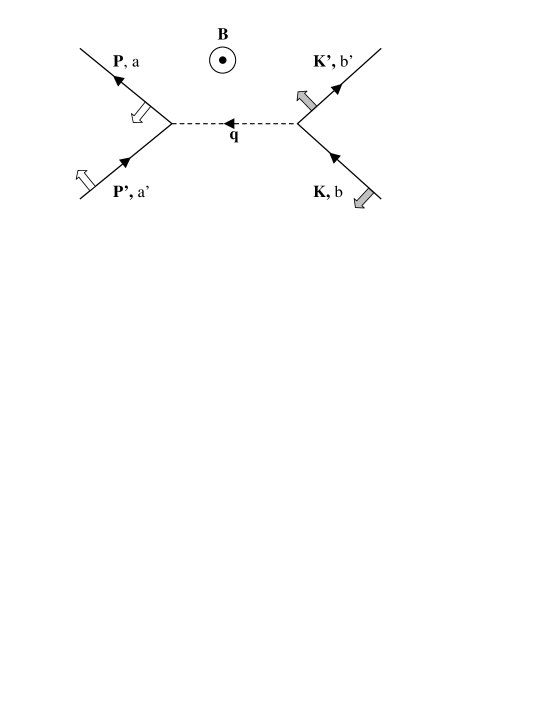
FIG. 1.: A sketch of a scattering event between exciton dipoles. One of the exciton-particles makes the transition $\{{\bf P}^{\prime},a^{\prime}\}\rightarrow\{{\bf P},a\}$, while the other one changes $\{{\bf K},b\}\rightarrow\{{\bf K}^{\prime},b^{\prime}\}$. Notice that in-plane dipole moments are perpendicular to each momentum, and they change upon scattering (as indicated by blank and shaded arrows). Dashed line indicates the momentum exchange due to the inter-exciton potential.

In these expressions, the functions $\phi(q)$, $\chi_{1}(q)$, and $\chi_{2}(q)$, are Fourier transforms of the dipolar interaction dependence on the center-of-mass coordinates, and are explicitly written in Appendix A. The in-plane “dipole moment” matrix elements are given formally by,

$${{\bf p}}_{\alpha^{\prime}\alpha}=\frac{2e}{i\gamma}\frac{\partial}{\partial{\bf q}}M_{\alpha^{\prime}\alpha}\,,$$ (24)

where $\hbar{\bf q}={\bf P}-{\bf P}^{\prime}$ as above, and the non-local “overlap” matrix elements are given by

$$M_{{\alpha^{\prime}}{\alpha}} = M_{n^{\prime}m^{\prime}{\bf P}^{\prime},nm{\bf P}}$$ (25)

$$= e^{i\frac{\gamma}{2}{\bf q}\cdot{\bf r}_{{\bf P}^{\prime}}}\int{e^{i\frac{\gamma}{2}{\bf q}\cdot{\bf r}}\,\Phi_{n^{\prime}m^{\prime}}^{*}({\bf r})\,\Phi_{nm}({\bf r}-{\bf u})}\,d^{2}{\bf r}\,,$$ (26)

with similar expressions for ${\bf p}_{\beta\beta^{\prime}}$ and $M_{\beta\beta^{\prime}}$. In the last equation, we have used ${\bf u}={\bf r}_{{\bf P}}-{\bf r}_{{\bf P}^{\prime}}$, and the gradient in Eq. (24) refers to the explicit $q$-dependence shown in (26), different from ${\bf u}$.

In the following sections, we describe typical features of the overlap and dipole matrices, $M_{\alpha\alpha^{\prime}}$ and ${\bf p}_{\alpha\alpha^{\prime}}$.

A Dipole matrix elements

In order to better understand the nature of the residual interaction matrices, we evaluate some of the lowest elements. In what follows, and for notational convenience, we use $\alpha=\{nm{\bf P}\}=\{a{\bf P}\}$, with $a$ standing for the indices of the $\Phi_{nm}$ states, so that one can write for example,

$${\bf p}_{\alpha^{\prime}\alpha} = {\bf p}_{a^{\prime}{\bf P}^{\prime},a{\bf P}}={\bf p}_{a^{\prime}a}({\bf P}-{\bf P}^{\prime},{\bf P}+{\bf P}^{\prime})={\bf p}_{a^{\prime}a}({\bf q},{\bf P}^{\prime})\,,$$ (27)

where the explicit dependence on the sum and difference of participating momenta is indicated. The last equality uses the overall conservation of magnetic momentum provided by the delta functions in (19) and (22).

The simplest dipole moment matrix element (for $a=\{00\}=a^{\prime}$) can be written as (see Appendix B),

$${{\bf p}}_{00{\bf P}^{\prime},00{\bf P}}={\bf p}_{00,00}({\bf q},{\bf P}^{\prime}) = \frac{e}{2}\left({\bf r}_{2{\bf P}^{\prime}+\hbar{\bf q}}+i\gamma r_{H}^{2}{\bf q}\right)\,e^{i\frac{\gamma}{4}{\bf q}\cdot{\bf r}_{2{\bf P}^{\prime}+\hbar{\bf q}}}\,e^{-(1+\gamma^{2})q^{2}r_{H}^{2}/8}\,,$$ (28)

where the in-plane momentum exchange ${\bf q}$, and the incoming magnetic momentum ${\bf P}^{\prime}$ are used to specify the dipole and non-local overlap matrix elements.

From this expression, the (non-interacting) long-wavelength limit ${\bf q}=0$ yields,

$${{\bf p}}_{00,00}({\bf q}=0,{\bf P}^{\prime}) = \frac{e}{2}{\bf r}_{2{\bf P}^{\prime}}=\frac{er^{2}_{H}}{\hbar}\left[\hat{z}\times{\bf P}^{\prime}\right]$$ (29)

$$= e{\bf r}_{{\bf P}^{\prime}}\,.$$ (30)

This represents what one could call the ‘proper’ dipole moment of the exciton in state $nm=00$, and with magnetic momentum ${\bf P}^{\prime}$, since the expectation value of the relative coordinate is ${\bf r}_{{\bf P}^{\prime}}$. In fact, it is possible to show (see Appendix B) that all the diagonal dipole matrix elements in the limit ${\bf q}\rightarrow 0$ yield ${\bf p}_{aa}({\bf q}=0,{\bf P})=e{\bf r}_{{\bf P}}$, since in fact all $\Phi_{nm}$ states have the same dipole moment (in this high field limit), as we discussed following Eq. (13). We emphasize that large momentum values correspond to larger exciton size and lower binding energy, as the exciton is increasingly polarized. [16] One expects that such high-${\bf P}$ states would be easily affected (even disintegrated) by perturbations in the system, such as impurities and surface inhomogeneities.

It is interesting to note the role that $\gamma=(m_{h}-m_{e})/M$ plays in Eq. (28), providing an imaginary part (or phase) proportional to ${\bf q}$ to the dipole matrix element. Notice further that for any $\gamma$ values, a non-vanishing momentum exchange ${\bf q}$ depresses exponentially the dipole matrix element, with a characteristic length $\approx r_{H}$. Since non-vanishing $q$ corresponds to the momentum/energy transfer from one exciton to the other, high momentum transfer processes will appear to be strongly suppressed by this potential. Let us discuss these features in the next section.

B Potential matrix elements

The simplest elements of the potential are those diagonal in the $\{a,a^{\prime}\}$ indices. For two excitons with incoming momenta ${\bf P}^{\prime}$ and ${\bf K}$ which exchange momentum ${\bf q}$, the potential matrix element is given by,

$$V_{00,00;00,00}({\bf q},{\bf P}^{\prime},{\bf K}) = \left\{\phi(q)\left[\frac{e^{2}}{4}({\bf r}_{2{\bf P}^{\prime}+\hbar{\bf q}}+i\gamma r^{2}_{H}{\bf q})\cdot({\bf r}_{2{\bf K}-\hbar{\bf q}}-i\gamma r^{2}_{H}{\bf q})+e^{2}d^{2}\right]+{\mathcal{V}}_{00,00;00,00}({\bf q},{\bf P}^{\prime},{\bf K})\right\}\times$$ (32)

$$\tilde{M}_{00,00}(-{\bf q},{\bf P}^{\prime})\tilde{M}_{00,00}({\bf q},{\bf K})$$

where,

$$\tilde{M}_{00,00}({\bf q},{\bf P}^{\prime})=\exp\left(i\frac{\gamma}{4}{\bf q}\cdot{\bf r}_{2{\bf P}^{\prime}+\hbar{\bf q}}-(\gamma^{2}+1)\frac{r^{2}_{H}q^{2}}{8}\right)\,,$$ (33)

and,

$${\mathcal{V}}_{00,00;00,00}({\bf q},{\bf P}^{\prime},{\bf K})=\frac{e^{2}}{4} \Big{\{} \Big{[}{\bf q}\cdot\Big{(}{\bf r}_{2{\bf P}^{\prime}+\hbar{\bf q}}+i\gamma r^{2}_{H}{\bf q}\Big{)}\Big{]}\Big{[}{\bf q}\cdot\Big{(}{\bf r}_{2{\bf K}-\hbar{\bf q}}-i\gamma r^{2}_{H}{\bf q}\Big{)}\Big{]}\chi_{1}(q)$$ (35)

$$-\Big{(}{\bf r}_{2{\bf P}^{\prime}+\hbar{\bf q}}+i\gamma r^{2}_{H}{\bf q}\Big{)}\cdot\Big{(}{\bf r}_{2{\bf K}-\hbar{\bf q}}-i\gamma r^{2}_{H}{\bf q}\Big{)}\chi_{2}(q)\Big{\}}\,.$$

Notice that these expressions contain a contribution from the constant $z$-component of the dipole moment, $ed$, as well as from the in-plane components.

From these equations, and considering the ${\bf q}\rightarrow 0$ limit of the potential (see Appendix A), we may write

$$V_{00,00;00,00}({\bf q}\to 0,{\bf P}^{\prime},{\bf K})=\frac{e^{2}}{2\sqrt{\pi}d\kappa}\left\{\left(1-6\,{\pi}^{3/2}\,\Gamma(3/4)\right)\,{\bf r}_{{\bf P}^{\prime}}\cdot{\bf r}_{{\bf K}}+d^{2}\right\}\,.$$ (36)

This result is expressed in terms of the proper dipole moment of each exciton, proportional to ${\bf r}_{{\bf P}^{\prime}}$ and ${\bf r}_{{\bf K}}$, as intuitively expected by Lerner and Lozovik. [16] It is clear that the sign of the first term in the interaction (36) depends on the relative orientations of ${\bf P}^{\prime}$ and ${\bf K}$, and the resulting dipole moments. The total interaction between excitons will be more/less repulsive for anti/parallel ${\bf P}^{\prime}$ and ${\bf K}$, as the contribution to the $z$-axis moment is modulated by the in-plane component. For small and moderate magnetic moment values, typical of the excitons in this system at low temperatures, the repulsive interaction is however only weakly modulated, since $d\gtrsim r_{2{\bf P}}=r^{2}_{H}P$, but it is still dependent on the relative orientation of the proper dipoles.

IV Scattering events

As we have mentioned, the potential matrix elements above allow the description of the collective excitations of the weakly repulsive gas of polarized excitons, in a manner similar to that treated in Ref. [[19, 20]]. Moreover, these potential expressions can also be used in a quantitative description of the kinematics of scattering events, as those needed in a treatment of the distribution function via the Boltzmann equation to evaluate drag,[21] or the evaluation of the Bose condensate properties in this dipole-interacting system.[22] As an illustration of their use, we describe in this section how the potential matrix elements calculated above can provide rates and cross sections for different inter-exciton scattering events. For simplicity, we deal here with ‘elastic’ collisions, when there is no change of the internal state under scattering. More complex events are in principle also allowed, although ‘inelastic’ processes are suppressed by the strong field.

If one considers scattering events in which the internal state of the excitons is left unchanged, one is then faced with a purely kinematically elastic collision. The description of this elastic collision, like any problem of two bodies, is simplified by changing to a system of coordinates in which the center of mass of the two particles is at rest. The scattering angle in the center of mass reference frame is denoted by $\theta$, and it is related to the angles $\theta_{1}$ and $\theta_{2}$ giving the scattering angles of the two particles in the laboratory system of coordinates. In the case in which the second particle was at rest before the collision, for example, one can write [17]

$$\tan\theta_{1}=\frac{m_{2}\sin\theta}{m_{1}+m_{2}\cos\theta}\,,\quad\quad\theta_{2}=\frac{1}{2}(\pi-\theta)\,,$$

where $m_{1}$, $m_{2}$ are the masses of the scattering objects. In our case, the masses of the two ‘particles’ (excitons) are the same ($m_{1}=m_{2}=M^{exc}_{a}$, which depends on the internal state $a=\{nm\}$), and we have simply,

$$\theta_{1}=\frac{1}{2}\theta\,,\quad\quad\theta_{2}=\frac{1}{2}(\pi-\theta)\,;$$

so that the particles diverge at right angles in the laboratory frame.

The scattering cross-section can be calculated using the Born approximation, since the residual potential (14), may be considered a weak perturbation. Notice, furthermore, that the residual potential depends only on the distance between excitons ${\bf x}-{\bf x}^{\prime}$, so that the scattering field is central. Now, in the center of mass frame of reference, we can write

$${\bf P}^{\prime}_{CM}={\bf n}\qquad\qquad{\bf K}_{CM}=-{\bf n}\,,$$ (37)

where ${\bf n}=({\bf P}^{\prime}-{\bf K})/2$, is the relative magnetic momentum between excitons. Thus, the interaction potential matrix element for this event, where the internal state is assumed to be $a=\{00\}$ before and after the collision, can be written as

$$V_{00,00;00,00}^{CM}({\bf q},{\bf n}) = \frac{e^{2}}{4}\left\{4\phi(q)d^{2}-\Big{[}\chi_{2}(q)-\phi(q)\Big{]}\Big{(}{\bf r}_{2{\bf n}+\hbar{\bf q}}+i\gamma r^{2}_{H}{\bf q}\Big{)}^{2}-\Big{(}{\bf q}\cdot{\bf r}_{2{\bf n}}+i\gamma r^{2}_{H}{\bf q}^{2}\Big{)}^{2}\chi_{1}(q)\right\}\times$$ (39)

$$e^{-(\gamma^{2}+1)\frac{r^{2}_{H}q^{2}}{4}}\,,$$

where $\hbar{\bf q}={\bf P}-{\bf P}^{\prime}={\bf K}-{\bf K}^{\prime}$. Other internal states are given by a different detailed expression, but identical kinematics (Appendix B).

In the case under consideration, Eq. (39) describes the matrix element for a ‘transition’ (scattering event) from a state with momentum ${\bf n}$ to the state with momentum ${\bf n}^{\prime}=({\bf P}-{\bf K}^{\prime})/2={\bf n}+\hbar{\bf q}$, which we could then denote as $U_{nn^{\prime}}$. Correspondingly, the scattering rate can be calculated from the golden rule,

$$dW_{fi}=(2\pi/\hbar)|U_{nn^{\prime}}|^{2}\delta(E_{n}^{\prime}-E_{n})\,,$$ (40)

where the final and initial energies of the exciton of interest are,

$$E_{n}^{\prime}-E_{n}=({\bf n}^{\prime 2}-{\bf n}^{2})/2M^{exc}_{00}\,,$$ (41)

where $M^{exc}_{00}$ is the effective excitonic mass of state {00}, including the electron-hole interaction, for $|{\bf n}|,|{\bf n}^{\prime}|\ll\hbar/r_{H}$. [16] The presence of the delta function in (40) indicates that the scattering event is kinematically elastic.

V Conclusions

We have presented explicit expressions for the residual interaction between polarized excitons in strong magnetic fields. This potential would have important consequences on the description of individual scattering events, as discussed, and the collective excitations of the system. Unfortunately, it is not clear how one would perform experiments to directly measure the many different scattering processes possible. Although we are hopeful that some experiments might be designed in the future to analyze these processes, we believe that the more direct probe would be study of the various collective modes in this interesting and unusual system. Since the density-fluctuation modes are now able to include rather complex internal excitations, the resulting modes may indeed be quite unusual and complicated. One would use the potential derived here in an approach similar to the case with no field, [19, 20] and results will be presented elsewhere.

We trust that these expressions would also be useful in the description of other kinematic and thermodynamic properties of the system.

A Potential functions

Because of the spurious short-range divergence introduced by the $|{\bf x}-{\bf x}^{\prime}|^{-3}$ dependence on the dipolar potential, we use the physical cutoff parameter provided by the finite $z$-direction polarization of the exciton $d$. [19] Therefore, by introducing the regularization factor as per $|{\bf x}-{\bf x}^{\prime}|^{-3}\rightarrow|{\bf x}-{\bf x}^{\prime}|^{-3}(1-e^{-|{\bf x}-{\bf x}^{\prime}|^{2}/d^{2}})$, we preserve the long-range dipolar interaction, while allowing for the short-range Coulomb-like repulsion. Correspondingly, we may write, with ${\bf S}={\bf x}-{\bf x}^{\prime}$,

$$\phi(q) = \frac{1}{\kappa}\int\,e^{i{\bf q}\cdot{\bf S}}\frac{1}{S^{3}}(1-e^{-S^{2}/d^{2}})\,d^{2}{\bf S}$$ (A1)

$$= \frac{q}{2\pi\kappa}\left\{-1+\frac{qd\sqrt{\pi}}{4}e^{-q^{2}d^{2}/8}\left[I_{1}\left(\frac{q^{2}d^{2}}{8}\right)+\left(1+\frac{4}{q^{2}d^{2}}\right)I_{0}\left(\frac{q^{2}d^{2}}{8}\right)\right]\right\}\,,$$ (A2)

where $I_{n}$ is the Bessel function of imaginary argument. Notice, incidentally, that

$$\phi(q\rightarrow 0)=\frac{1}{2\kappa d\sqrt{\pi}}\,,$$ (A3)

and is therefore ill-defined for $d=0$. This function $\phi(q)$ accounts for the first term in the interaction in Eq. (22) or (32).

Similarly, the second dipolar term can be written as

$$I^{(2)} = \frac{1}{\kappa}\int e^{i{\bf q}\cdot{\bf S}}\frac{({\bf p}\cdot{\bf S})({\bf p}^{\prime}\cdot{\bf S})}{S^{5}}(1-e^{-S^{4}/d^{4}})\,d^{2}{\bf S}$$ (A4)

$$= \frac{1}{\kappa}\left({\bf p}\cdot\frac{1}{i}\frac{\partial}{\partial{\bf q}}\right)\left({\bf p}^{\prime}\cdot\frac{1}{i}\frac{\partial}{\partial{\bf q}}\right)\int e^{i{\bf q}\cdot{\bf S}}\frac{1-e^{-\frac{S^{4}}{d^{4}}}}{S^{5}}\,d^{2}{\bf S}$$ (A5)

$$= ({\bf p}\cdot{\bf q})({\bf p}^{\prime}\cdot{\bf q})\chi_{1}(q)-\chi_{2}(q)\,{\bf p}\cdot{\bf p}^{\prime}\,,$$ (A6)

where for $qd\gg 1$

$$\chi_{1}(q)=\frac{3}{\kappa}\sum_{k=0}^{\infty}{\frac{2\pi(-256)^{k}(4k+1)(4k+3)\Gamma^{2}(k+\frac{1}{4})\Gamma^{2}(k+\frac{3}{4})}{\Gamma^{2}(\frac{1}{4})\Gamma^{2}(\frac{3}{4})(k+1)!d^{4k+4}q^{4k+5}}}$$ (A7)

and

$$\chi_{2}(q)=\frac{3}{\kappa}\sum_{k=0}^{\infty}{\frac{2\pi(-256)^{k}(4k+1)\Gamma^{2}(k+\frac{1}{4})\Gamma^{2}(k+\frac{3}{4})}{\Gamma^{2}(\frac{1}{4})\Gamma^{2}(\frac{3}{4})(k+1)!d^{4k+4}q^{4k+3}}}$$ (A8)

On the other hand, for $qd\ll 1$, Eq. (A6) behaves as,

$$I^{(2)}=-\frac{3\pi\Gamma(3/4)}{\kappa d}{\bf p}\cdot{\bf p}^{\prime}\,.$$ (A9)

B Dipole matrix elements

Notice that the dipole moment matrix elements obey the symmetry relation

$${{\bf p}}_{nm{\bf P},n^{\prime}m^{\prime}{\bf P}^{\prime}}={{\bf p}}^{*}_{n^{\prime}m^{\prime}{\bf P}^{\prime},nm{\bf P}}\,.$$ (B1)

Some special cases of overlap and dipole moment matrix elements follow. For the diagonal elements,

$$M_{00{\bf P}^{\prime},00{\bf P}}=\exp\left[{}^{i\frac{\gamma}{4}{\bf q}\cdot({\bf r}_{{\bf P}}+{\bf r}_{{\bf P}^{\prime}})-\frac{u^{2}}{8r_{H}^{2}}-\frac{\gamma^{2}r_{H}^{2}q^{2}}{8}}\right]\,,$$ (B2)

where ${\bf u}={\bf r}_{{\bf P}}-{\bf r}_{{\bf P}^{\prime}}$, and

$${{\bf p}}_{00{\bf P}^{\prime},00{\bf P}}=\frac{e}{2}\left({\bf r}_{{\bf P}}+{\bf r}_{{\bf P}^{\prime}}+ir_{H}^{2}\gamma{\bf q}\right)\,e^{i\frac{\gamma}{4}{\bf q}\cdot({\bf r}_{{\bf P}}+{\bf r}_{{\bf P}^{\prime}})-(\gamma^{2}+1)\frac{r_{H}^{2}q^{2}}{8}}$$ (B3)

$$=\frac{e}{2}\left({\bf r}_{{\bf P}}+{\bf r}_{{\bf P}^{\prime}}+ir_{H}^{2}\gamma{\bf q}\right)\tilde{M}_{00{\bf P}^{\prime},00{\bf P}}$$ (B4)

The simplest/lowest off-diagonal elements are,

$$M_{01{\bf P}^{\prime},01{\bf P}}=\left(1-\frac{\gamma^{2}r_{H}^{2}q^{2}}{8}-\frac{u^{2}}{8r_{H}^{2}}+\frac{\gamma}{4}\,{\bf u}\times{\bf q}\cdot\hat{\bf z}\right)M_{00{\bf P}^{\prime},00{\bf P}}\,,$$ (B5)

and

$${{\bf p}}_{01{\bf P}^{\prime},01{\bf P}}=\left[1-r_{H}^{2}q^{2}\left(\frac{\gamma^{2}}{8}+\frac{\gamma}{4}+1\right)\right]{{\bf p}}_{00{\bf P}^{\prime},00{\bf P}}+i(\gamma+1)\frac{er_{H}^{2}{\bf q}}{2}\tilde{M}_{00{\bf P}^{\prime},00{\bf P}}\,.$$ (B6)

Similarly,

$$M_{0-1{\bf P}^{\prime},0-1{\bf P}} = \left(1-\frac{\gamma^{2}r_{H}^{2}q^{2}}{8}-\frac{u^{2}}{8r_{H}^{2}}-\frac{\gamma}{4}\,{\bf u}\times{\bf q}\cdot\hat{\bf z}\right)M_{00{\bf P}^{\prime},00{\bf P}}\,,$$ (B7)

$${{\bf p}}_{0-1{\bf P}^{\prime},0-1{\bf P}} = \left[1-r_{H}^{2}q^{2}\left(\frac{\gamma^{2}}{8}+\frac{\gamma}{4}+\frac{1}{8}\right)\right]{{\bf p}}_{00{\bf P}^{\prime},00{\bf P}}+i(\gamma-1)\frac{er_{H}^{2}{\bf q}}{2}\tilde{M}_{00{\bf P}^{\prime},00{\bf P}}\,;$$ (B8)

$$M_{00{\bf P}^{\prime},01{\bf P}} = \frac{1}{\sqrt{2}}\left(i\frac{\gamma r_{H}qe^{-i\varphi_{q}}}{2}-\frac{ue^{-i\varphi_{u}}}{2r_{H}}\right)M_{00{\bf P}^{\prime},00{\bf P}}\,,$$ (B10)

$${{\bf p}}_{00{\bf P}^{\prime},01{\bf P}} = i\frac{\gamma+1}{2\sqrt{2}}r_{H}[{\bf q}\cdot(\hat{\bf x}-i\hat{\bf y})]{{\bf p}}_{00{\bf P}^{\prime},00{\bf P}}+\frac{er_{H}}{\sqrt{2}}(\hat{\bf x}-i\hat{\bf y})\tilde{M}_{00{\bf P}^{\prime},00{\bf P}}\,;$$ (B11)

$$M_{00{\bf P}^{\prime},0-1{\bf P}} = \frac{1}{\sqrt{2}}\left(i\frac{\gamma r_{H}qe^{i\varphi_{q}}}{2}-\frac{ue^{i\varphi_{u}}}{2r_{H}}\right)M_{00{\bf P}^{\prime},00{\bf P}}\,,$$ (B13)

$${{\bf p}}_{00{\bf P}^{\prime},0-1{\bf P}} = i\frac{\gamma-1}{2\sqrt{2}}r_{H}[{\bf q}\cdot(\hat{\bf x}+i\hat{\bf y})]{{\bf p}}_{00{\bf P}^{\prime},00{\bf P}}+\frac{er_{H}}{\sqrt{2}}(\hat{\bf x}+i\hat{\bf y})\tilde{M}_{00{\bf P}^{\prime},00{\bf P}}\,;$$ (B14)

$$M_{01{\bf P}^{\prime},0-1{\bf P}} = -\left(\frac{\gamma^{2}r_{H}^{2}q^{2}e^{i2\varphi_{q}}}{8}+\frac{u^{2}e^{i2\varphi_{u}}}{8r^{2}_{H}}\right)M_{00{\bf P}^{\prime},00{\bf P}}\,,$$ (B16)

$${{\bf p}}_{01{\bf P}^{\prime},0-1{\bf P}} = -(\gamma^{2}+1)\frac{r^{2}_{H}q^{2}e^{i2\varphi_{q}}}{8}{{\bf p}}_{00{\bf P}^{\prime},00{\bf P}}+i\frac{er^{2}_{H}qe^{i\varphi_{q}}}{\sqrt{2}}(\hat{\bf x}+i\hat{\bf y})\tilde{M}_{00{\bf P}^{\prime},00{\bf P}}\,.$$ (B17)

REFERENCES

- [1] V. G. Kogan and B. A. Tavger, in Physics of p-n junctions and semiconductor devices, Eds. S. M. Ryvkin and Yu. V. Smartsev, (Nauka, Leningrad, 1969), p. 37.
- [2] Yu. E. Lozovik, and V. I. Yudson, Zh. Eksp. Teor. Fiz. 71, 738 (1976) [Sov. Phys. JETP 44, 389 (1976)]; JETP Lett. 22, 274 (1975).
- [3] S. I. Shevchenko, Fiz. Nizk. Temp. 2 505 (1976) [Sov. J. Low Temp. Phys. 2, 251 (1976)].
- [4] S. I. Shevchenko, Phys. Rev. B 56, 10355 (1997)
- [5] A. B. Dzyubenko, JETP Lett. 66, 617 (1997), and references therein.
- [6] Yu. E. Lozovik, O. L. Berman, and V. G. Tsvetus, Phys. Rev. B59, 5627 (1999).
- [7] T. Fukuzawa, E. E. Mendez and J. M. Hong, Phys. Rev. Lett. 64, 3066 (1990).
- [8] J. A. Kash, M. Zachau, E. E. Mendez, J. M. Hong, T. Fukuzawa, Phys. Rev. Lett. 66, 2247 (1991)
- [9] V. Negoita, D. W. Snoke, and K. Eberl, Phys. Rev. B 60, 2661 (1999).
- [10] L. V. Butov, A. Zrenner, G. Abstreiter, G. Böhm, and G. Weimann, Phys. Rev. Lett. 73, 304 (1994).
- [11] J. Kono, B. D. McCombe, J.-P. Cheng, I. Lo, W. C. Mitchell, and C. E. Stutz, Phys. Rev. B 55, 1617 (1997).
- [12] P. F. Vohralik, R. O. Watts, and M. H. Alexander, J. Chem. Phys. 93, 3983 (1990), and references therein.
- [13] N. Read, Phys. Rev. B 58, 16262 (1998).
- [14] P.Y. Yu and M. Cardona, Fundamentals of Semiconductors (Springer Verlag, New York, 1996)
- [15] L. P. Gor’kov and I. E. Dzyaloshinskiĭ, Sov.Phys. JETP 26, 449 (1968).
- [16] I. V. Lerner and Yu. E. Lozovik, Sov. Phys. JETP 51, 588 (1980).
- [17] L. D. Landau and E. M. Lifshitz, Quantum Mechanics (Pergamon, New York, 1977).
- [18] H. Ehrenreich and M. H. Cohen, Phys. Rev. 115, 786 (1959).
- [19] D. M. Kachintsev and S. E. Ulloa, Phys. Rev. B 50, 8715 (1994).
- [20] R. A. Vazquez-Nava, S. E. Ulloa, and M. del Castillo-Mussot, Phys. Status Sol., to appear (2000).
- [21] Yu. E. Lozovik and M. V. Nikitov, J. Experim. Theor. Phys. 89, 775 (1999).
- [22] K. Goral, K. Rza̧zewski, and T. Pfau, Phys. Rev. A61, 051601 (2000); L. Santos, G.V. Shlyapnikov, P. Zoller, and M. Lewenstein, cond-mat/0005009.