Sharp interface limit of a phase-field model of crystal grains
Abstract
We analyze a two-dimensional phase field model designed to describe the dynamics of crystalline grains. The phenomenological free energy is a functional of two order parameters. The first one reflects the orientational order while the second reflects the predominant local orientation of the crystal. We consider the gradient flow of this free energy. Solutions can be interpreted as ensembles of grains (in which the phase of the order parameter is approximately constant in space) separated by grain boundaries. We study the dynamics of the boundaries as well as the rotation of the grains. In the limit of the infinitely sharp interface, the normal velocity of the boundary is proportional to both its curvature and its energy. We obtain explicit formulas for the interfacial energy and mobility and study their behavior in the limit of a small misorientation. We calculate the rate of rotation of a grain in the sharp interface limit and find that it depends sensitively on the choice of the model.
pacs:
81.10.Aj, 81.30.-t, 81.10.Jt, 61.72.MmI Introduction
The characterization and evolution of microstructure forms a cornerstone of materials science. In particular the grain structure of a polycrystalline material determines many of its properties. Recent efforts at modeling the evolution of grain boundaries have used a variety of approaches Morin , Lusk , Chen , Holm . Herein we focus on the recently introduced phase field model of Kobayashi, Warren and Carter (KWC)kwc3 which is based on earlier attempts by the same authors (kwc and wkc ).
The model is motivated by symmetry principles and has a surprisingly rich set of physical characteristics. In particular, KWC showed numerically that solutions to this model can be interpreted as a collection of grains. The velocity of the interface between the grains was found to be approximately proportional to the local curvature of the interface, but the grains were also able to rotate towards lower energy misorientations. In support of the notion of grain rotation, three independent unpublished molecular dynamics studies by M. Upmanyu and D. Srolovitz, S. R. Phillpot and D. Wolf, and S. Srivillaputhur and J. W. Cahn, suggest that grain rotation will occur under certain circumstances. In addition, there is a substantial history (and debate) concerning the mechanisms Li , Martin and observation of grain rotation King ; chen_balluffi .
The KWC phase field model is challenging mathematically because of a singular term in the free energy. Kobayashi and Giga kg99 studied similar singular models and showed that there is a way to handle the singularity consistently. In this paper we will apply their method to the KWC model and show that its solutions can indeed be interpreted as grains. Our main goal is to analytically obtain the properties of a grain boundary as well as the rotation rate of a grain. We accomplish this task by considering a distinguished limit of the model parameters in which the width of the boundary vanishes while its measurable characteristics remain finite and non-zero. The methodology of this this so called sharp interface limit is well established Caginalp , Mcfadden , fife .
The organization of this paper is as follows. In Sec. II we introduce the order parameters, phenomenological free energy, and the gradient flow equations. We next perform a formal asymptotic expansion of the model in Sec. III. The zeroth order probelm of this expansion is discussed in Sec. IV, where we obtain the profile and the energy of the static flat boundary. In the following section (Sec. V) the first order asymptotics are examined. We are able to determine the velocity of a curved grain boundary. We find that this velocity is proportional to both the curvature and the interfacial energy and obtain an expression for the mobility of the interface. As noted above, grains can rotate in this model. We calculate the rate of rotation of a grain in Sec. VI. Finally, in Sec. VII we apply all of the results described herein to the simple case of a circular grain embedded in a matrix. In our conclusion we discuss further ideas and the implications of this phase field model for the problem of coarsening in polycrystals in Sec. VIII.
II Model
We model the evolution of a collection of nearly perfect crystalline grains in two dimensionsvia a phase field model. First, we discuss order parameters which capture the microscopic physics of grain boundaries. It is then possible to construct a phenomenological free energy which favors a perfect uniform crystal and supports stable grain boundaries. Evolution of an ensemble of grains is then modeled via gradient flow of this free energy.
Following kwc3 we develop two order parameters which capture the physics of grain boundaries. To distinguish grains of different orientations we introduce a continuously varying local orientation . Since the energy of crystal does not depend on itself, the phenomenological free energy will be a functional of the gradients of only. The second order parameter is used to differentiate the nearly perfect crystal in the interior of the grains from the disordered material in the grain boundary. It varies from perfect order to complete disorder . Both order parameters are not conserved.
We analyze the free energy (based on KWC)
| (1) |
where , and are positive model parameters. Some readers may find the overall prefactor of suggestive. Subsequently we will examine the limit . This prefactor ensures that the surface energy of a grain boundary tends to a non-zero constant.
Term by term, the above free energy deserves some discussion, although the reader interested in the full motivation of this model is referred to kwc3 . The first term describes the penalty for gradients in the order parameter (grain boundaries cost energy). The free energy density is chosen to be a single well with the minimum at and reflecting the fact that disordered material has higher free energy. The third and fourth terms are an expansion in , where the couplings and must be positive definite. KWC argued that the expansion in must begin at first order to assure the existence of stable grain boundaries. This term yields a singularity in the dynamic equations.
Indeed, Ref. kwc3 omitted the term in their analytical investigation of a stationary flat interface. This term was added in kwc , for practical reasons, in order to solve the model numerically. We shall see that this term makes no qualitative difference in the properties of static grain boundaries. However, as shown in Sec. V.1, the mobility of a grain boundary vanishes as when in the limit. Thus, the extra term introduced in KWC seems to be required for grain boundaries to move.
Assuming relaxational dynamics for a non-conserved set of order parameters, we find the gradient flow equations:
where we used the subscript to denote differentiation. The mobility functions and must be positive definite, continuous at , but are otherwise unrestricted. The system (2) must be supplemented by initial and boundary conditions and a rule that specifies the handling of the indeterminancy (and sigular divergence) of the term . This particular type of the singularity is generally handled in a theory of extended gradients. Ref. kg99 proves that there is indeed a unique way to prescribe the value of the right hand side of Eq. (2) when . While we do not wish to attempt to explain all of the details of Ref. kg99 , it is useful to summarize the ultimate conclusion of the mathematical analysis. Thus, let us define a collection of distinct connected regions where . We shall refer to as the interior of grain . The essence of the method of dealing with the singularity is that the orientation must remain uniform in space in each . Therefore, the right hand side of Eq. (2) is chosen in to be uniform in . This condition, along with the requirement that , and be continuous at the boundaries of , uniquely determines the rotation rate of each grain (i.e. in each ) and the motion of its boundaries.
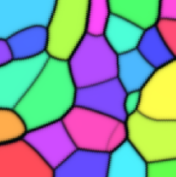
Ref. 2d_sim verifies numerically that typical solutions of the gradient flow system (2) indeed consist of a collection of connected regions in which and (grain interiors) separated by narrow regions (grain boundaries) in which the orientation changes smoothly between the neighboring grains. Thus, the grains rotate ( changes in time uniformly in each grain), and grain boundaries migrate (see Fig. 1 adopted from Ref. 2d_sim ).
III Formal asymptotics
Having elucidated the general properties of the model, we now examine the sharp-interface limit, in order to extract the physical quantities from our phase field model. As discussed earlier, solutions to the extended gradient flow system (2) consist of grains in which separated by a network grain boundaries in which . Although no rigorous proof of the inevitability of this solution structure exists, there are two plausibility arguments. First, once this structure develops, one can show that it will persist kg99 . And second, such a solution can be explicitly found for a flat stationary interface between two grains shown schematically in Fig. 2. This case corresponds to the zeroth order of the formal asymptotic expansion as we show in what follows.

Fig. 2 is highly suggestive. We have a bicyrstalline system with a localized region where properties change (i.e. the grain boundary). Let us therefore consider the limit of the gradient flow system (2). We expect the width of the grain boundary region, defined by , to shrink to zero. We employ the standard method of matched asymptotics fife which uses the small ratio of the interface width to its radius of curvature as an expansion parameter. In this limit, all functions and their derivatives vary slowly along the interface compared to their variation across the interface. The analysis can therefore be advanced by defining a coordinate normal to the interface and scaling it by . The order parameters as functions of this new coordinate are termed the inner solution. They are expanded into a power series in and the resulting hierarchy of equations is solved order by order, subject to a matching condition with the outer solution. This outer solution, obtained by setting to zero, is valid far away from the interface.
The mathematics of the sharp interface limit of our model is atypical because the fields and obey two different sets of equations kg99 . Eqs. (2) hold in the grain boundary region which is defined as a strip between two smooth non-intersecting curves and (see Fig. 3). Outside this strip and
| (3) |
Following cahn_fife , let us adopt curvilinear orthogonal coordinate system . Let be the distance of the point in from . On , coordinate is the arc length. We introduce a scaled variable , and expand and in a formal power series in
| (4a) | |||||
| (4b) | |||||
This expansion is valid in and its immediate neighborhood. Also fife
| (5a) | |||||
| (5b) | |||||
| (5c) | |||||
where is the unit vector normal to pointing into ( increases in the direction of ) and is the unit vector along the lines of constant . The curvature is positive when points away from the center of curvature of . Normal velocity is positive when the interface moves in the direction of . This configuration is shown in Fig. 3.

In order to proceed we must fix the scaling of , , and in the sharp interface limit. We select the scaling for which 1) a flat interface does not move, and 2) all terms in the free energy Eq. (1) scale with the same power of . We also assume that the mobility functions and are independent of in the sharp interface limit. These conditions fix
| (6) |
The final ingredient of the formal asymptotic analysis is the matching of the inner and outer solutions. The inner solution is found separately in the grain boundary () and in its immediate neighborhood (). The inner solution valid in is denoted by and without superscripts. The piece of the inner solution valid in the interior of a grain just outside of is denoted by and . It is matched with the outer solution and for . We must also match the two pieces of the inner solution and their derivatives at the boundaries of the strip which are at .
IV Zeroth order solutions: interface width and energy
Now, having detailed the formal method of asymptotic expansion, we proceed to examine the results of this expansion, term by term. We begin, naturally enough, with the zeroth order. The ultimate result of the zeroth order calculation with be a determination of (i) the interface width (ii) the surface energy and (iii) the value of the order parameter in grain boundary.
Without loss of generality we can shift the origin of so that it is in the middle of , . We first look at the grain interior region . Substituting the scaling ansatz Eq. (6) and the -expansion (4) into (2) and using (5) we obtain
| (7) |
These solutions must be matched with the outer solution and , as . Since the zeroth order functions and are independent of , the coordinate along the interface, and time , they describe a flat stationary interface. They should therefore be symmetric with respect to the center of the boundary . We can thus set , half the total misorientation (which is in general a function of time). Using the fact that we arrive at
| (8) |
After similar manipulations we obtain the equations valid in for
| (9a) | |||||
| (9b) | |||||
Note that we assumed that in . This assumption proves to be unrestrictive since all measurable quantities depend on the square of this derivative.
To obtain the boundary conditions for and we employ two ideas. First, due to the aforementioned symmetry, is even and is odd in . Second, the requirement that , and their derivatives be continuous at can be shown to lead to the continuity of all terms in the -expansion (4) at . We thus obtain
| (10) | |||
| (11) |
where . Let us also introduce . This designation reflects our assumption that in so that . We can prove that, in particular cases, this assumption is indeed justified.
Using the last boundary condition we integrate (9b) to obtain
| (12) |
Upon substitution of this expression into Eq. (9a) we discover that is an integrating factor. Using the second condition in Eq. (10) we obtain
| (13) |
The first condition in Eq. (10) furnishes the relation between and
| (14) |
Armed with this condition we can obtain an equation for via
| (15) |
where we took advantage of the monotonicity of . Once is found we can calculate the width of the boundary
| (16) |
and the interfacial energy
| (17) |
Remarkably, these formulas reduce the flat boundary problem to quadratures. We are able to compute and from Eqns. (14) and (15), the interface width from Eqn. (16), and the surface energy from Eqn. (17).
As useful as these expressions are, insight can be better obtained from analytic expressions, since the above four equations must typically be solved numerically. Thus, let us examine the behavior of the zeroth order solution in certain limits in which an approximate solution can be found. The integral on the right hand side of Eq. (15) can be calculated approximately when it is small. We identify two such situations.
IV.1 Small approximation to the zeroth order solution
To make contact with Ref. kwc3 in which the term in the free energy is set to zero, we consider a limit in which its coefficient vanishes . Expanding Eq. (14) in powers of we obtain to lowest order
| (18) |
where , etc. Thus, as , the difference between and vanishes, while they remain well separated from . Therefore, , and and their derivatives are regular at the undistinguished point .
Let us define an auxiliary parameter via and expand Eq. (15) in powers of . We obtain
| (19) |
One could in principle now invert (19) to solve for . The width of the boundary can be then found with the same accuracy
| (20) |
The interfacial energy is, in this same approximation,
| (21) |
For a special case examined in Ref. kwc3 , , , and , Eq. (19) is easily invertible. Indeed, the expressions for and coincide with those of Ref. kwc3 .
We finally remark that within this approximation, the behavior of and in the limit of small misorientation depends on the properties of and near . To see why this is true, let us look at Eq. (19) in the limit of small . Unless is singular at some value of other than (unphysical), small implies small since . We shall see in the next subsection that it is true in general. This fact is not surprising since small angle boundaries can be thought of as arrays of distant dislocations.
IV.2 Small approximation to the zeroth order solution
All parameters being fixed, the right hand side of Eq. (15) can be small if and only if
| (22) |
Since , it is clear from Eq. (14) that
| (23) |
Also, since we chose we can approximate it by a parabola near . Then
| (24) |
If the behavior of and near is known, we can obtain a complete solution to the zeroth order problem in this limit. Instead let us focus on the scaling of the interface width and the interfacial energy in the limit. This scaling can be deduced without a complete solution of the zeroth order problem.
Suppose that near ()
| (25) |
Then from (24) we obtain
| (26) |
Note that since by definition, the scaling exponent in Eq. (26) must be greater than or equal to . This means that in this limit, the zeroth order solution exists only when .
To determine the scaling of the right hand side of Eq. (15) we define a finite integration variable via . Then
| (27a) | |||||
| (27b) | |||||
| (27c) | |||||
We used the fact that to establish that the second term in the square brackets of (27c) dominates (when all three terms in these square brackets are equally important). Substituting scaling relations (27) into Eq. (15) we obtain
| (28) |
We are now ready to calculate the behavior of and in the limit. Substituting the scaling relations (27) into (16) we obtain
| (29) |
The interfacial energy consists of three pieces which scale differently with . We list them separately
| (30b) | |||||
| (30c) | |||||
We can make several observations. First, since , always dominates in the limit. Second, when we can integrate (25) to obtain . When , we obtain in a similar fashion . For the behavior of near is arbitrary. Thus, the scaling of the interfacial energy (whether it is dominated by or ) in the limit of the small misorientation can be freely controlled by adjusting the behavior of and near .
V First order solutions: interface mobility
Having completed our analysis of the zeroth order in the asymptotic expansion, we now continue on to first order. This order in the expansion will yield the velocity of the interface as a function of geometry, mobilities, and surface energy. From classical as well as order parameter models, we expect this motion to be by curvature AC , and, as we show below, this is indeed the case.
To begin, in order for us to establish the matching conditions between the two pieces of the first order solution, let us look at the equation for valid in
| (31) |
Progress can be made by noticing that is a solution of (31) with the left hand side set to . We can take advantage of this fact by multiplying Eq. (31) by and integrating over the grain interior. Using the matching condition with the outer solution which states that all derivatives vanish as , we obtain
| (32) |
As we mentioned before, all orders of the -expansion and their derivatives must be continuous at or, equivalently, at . Consequently, we may drop the superscript from the expression on the left hand side of Eq. (32). This condition will suffice to set at . We will not need the boundary condition for at .
Turning our attention to the boundary region we write down the first order equations
| (33a) | |||||
| (33b) | |||||
where we used the fact that . The couplings , , , and their derivatives, and , in Eqs. (33) are evaluated at the zeroth order solution.
We can fix the boundary conditions at for the first order functions by noticing that is odd while is even in . Therefore
| (34) |
Using the second condition we integrate (33b) to obtain
| (35) |
Upon substitution of this expression into (33a) we obtain an equation for of the form
| (36) |
where
| (37) |
The exact form of is unimportant since we can show by direct substitution that (as in a conventional asymptotic expansion problem) . This fact can be utilized to obtain a solvability condition which determines the velocity of the interface . Multiplying Eq. (36) by and integrating over we obtain
| (38) |
Solving for the interface velocity and using Eqs. (12), (13) and (17) yields
| (39) |
As expected, is proportional to both the curvature and the energy of the interface. The mobility is given by
| (40) |
We dropped the superscript since it is clear that solutions which are valid in the grain interior should be used in (40) for .
Just as in a conventional formal asymptotic analysis, we obtained the normal velocity of the interface without having to solve the first order equations. This is a general feature of analyses of this kind and allows one to express the mobility of the interface in terms of the properties of a stationary interface.
To better understand the behavior of the interface mobility , let us apply the approximations of sections IV.1 and IV.2 to Eq. (40).
V.1 Mobility in the small limit
To illustrate the importance of the term in the free energy for the motion of boundaries, let us again consider the limit in which its coefficient vanishes. The second term in Eq. (40) dominates in this limit. Assuming for the sake of the argument that does not depend on , we obtain
| (41) |
The mobility of the grain boundary therefore vanishes as in this limit in support of our claim that the term is required for migration of boundaries.
V.2 Mobility in the small limit
It is instructive to trace the behavior of the interface mobility in the limit of the vanishing misorientation. For simplicity we assume here that the mobility functions and are regular and assume a non-zero value at and . Using (27) we obtain the scaling of the three pieces which make up the right hand side of (40)
| (42a) | |||||
| (42b) | |||||
| (42c) | |||||
Eq. (28) can now be used to determine the behavior of in the limit. We obtain
| (43) |
To illustrate, if and are regular at so that our analysis yields while so that the interface velocity diverges in the limit of vanishing misorientation .
VI Grain rotation
As we discussed above, this model also allows for the grains to rotate. Let us consider a fully developed grain structure. In the sharp interface limit, the solution consists of a set of regions of spatially uniform (grains) separated by narrow (or order ) grain boundaries. To calculate the rotation rate of grain , we integrate Eq. (2) over the grain interior . We obtain
| (44) |
Here is the length of the common boundary between grains and . The summation is over the neighboring grains of orientation . In integrating by parts we used the continuity of at the edge of the grain kg99 . In the grain boundary , is a unit vector in the direction of increasing . Thus, away from a triple junction, on both edges of the boundary between grains and . The unit normal points from grain into grain . The periodicity of must be taken into account to calculate .
Recall that is exponentially close to in all of except a narrow (of order ) strip near the boundary. Therefore, if is neither a zero nor a singularity of , the integral on the left hand side of (44) is approximately equal to , where is the area of the -th grain. This choice of is problematic, however, since in the sharp interface limit . We therefore reach a remarkable conclusion that when is regular at , grain rotation dominates grain boundary migration in the sharp interface limit. The reason for this unexpected result is that is continuous across the edge of the grain boundary. Inside the grain boundary, this time derivative must scale with the inverse of the grain boundary width . The time rate of change of the orientation in the grain interior must therefore have the same scaling.
Another way of interpreting the divergence of the rotation rate in the sharp interface limit is to consider what happens in the interior of the grain. Since the orientation order parameter is constrained to remain uniform in space, it may be thought of as obeying a diffusion equation with infinite diffusivity. It is therefore not surprising that for a generic choice of the mobility function , the rotation rate is of the same order as the rate of change of in the grain boundaries (fast). The resolution of this paradox is in fact satisfyingly physical. When material is nearly a perfect crystal ( close to 1), i.e. there are few defects, one should expect the rate at which the order parameters change to vanish. This can be accomplished by letting the mobility functions and diverge at .
In fact, that for a particular choice of weakly singular the grain rotation rate no longer diverges in the sharp interface limit. The integral on the left hand side of (44) may be calculated approximately in the sharp interface limit. We will need an expression for far away from the boundary where it is close to . Using the approximation for , we obtain
| (45) |
Therefore, focusing on the -scaling in the sharp interface limit, we deduce that
| (46) |
where is some macroscopic length of the order of the grain size. Therefore no longer diverges in the sharp interface limit. Another important consequence of this argument is that since the perimeter of a grain is proportional to , the rotation rate is inversely proportional to
| (47) |
This prediction is independent of the choice of other the model functions. It is inconsistent with the heuristic derivations gessinger ; chen_balluffi of the rotation rate due to the diffusion of atoms along the grain boundary. These studies obtain a or scaling of depending on the mechanism. In a separate study, Martin Martin assumed that rotation is caused by viscous motion of dislocations and obtained a rotation rate which was independent of .
VII Approximate model of a single circular grain
To illustrate the predictions of the sharp interface limit calculation of the preceding sections, we consider a circular grain of radius and orientation embedded in an immovable matrix of orientation . To make analytical progress we choose , , , , to ensure finite rotation rate in the sharp interface limit and Read-Shockley readshockley behavior low angle boundaries. We also restrict ourselves to the small approximation.


In this limit we can carry out the expansion in detail to obtain
| (48) |
Applying the motion by curvature result (39) we obtain
| (49) |
where . The expression for the rotation rate with the radius of the grain and misorientation can be obtained via the arguments of this section above. We obtain
| (50) |
where . Solutions to these equations for and are given in Figs. 4 and 5. The ratio controls the behavior of the solution. When this ratio is small, rotation dominates the dynamics so that the radius of the grain is not significantly reduced by the time the grain rotates into alignment with the matrix. On the other hand, when this ratio is large, the evolution of the radius squared of the grain is almost linear in time as in the case of the motion by curvature.
VIII Discussion
In this paper we analyze a modified version of the phase field model of KWC kwc . This model is constructed to describe rotation of crystalline grains coupled to the motion of grain boundaries. The order parameter reflects the local crystal orientation, whereas represents local crystalline order. The Ginzburg-Landau free energy depends only on and is therefore invariant under rotations. Inclusion of the non-analytic term into the free energy results in singular gradient flow equations. However, this singularity can be dealt with in a systematic way.
Quite generally, solutions to the model represent a collection of regions of uniform —grains—connected by narrow (of order ) internal layers—grain boundaries. We are able to calculate the velocity of the boundaries in the limit of vanishing interface thickness, and find that it is proportional to the product of surface energy, curvature of the interface, and a mobility which depends on model parameters. The behavior of the interfacial width, energy and mobility in the limit of the small misorientation is controlled by the behavior of the model couplings near .
We calculate the rate of grain rotation in the sharp interface limit and find that it diverges unless the mobility function is singular at . For a logarithmic choice of this singularity, the rate of the grain rotation is finite and non-zero in the sharp interface limit. We explain this mathematical requirement by noting that the singular term in the free energy results in infinitely fast diffusion in the interior of a grain. Therefore, -dependent mobility must compensate for that fact. This logarithmically singular leads to the conclusion that the rotation rate of a grain scales with the inverse of its area. This is a robust prediction of our model independent of the choice of all other couplings.
For a plausible choice of model functions, motivated by the physics of low angle grain boundaries, we derive and solve equations describing a circular grain embedded in a matrix. We find that, as expected, when the scaled coefficient of the term in the free energy is large, rotation is fast so that the radius of the grain does not change much by the time the grain rotates into coincidence with the matrix. While when is small, rotation becomes important only when the radius is significantly reduced.
We conclude by remarking that the model may be readily generalized in a variety of ways. We may extend the model to three dimensions, by constructing an appropriate tensor order parameter which reflects the symmetries of the lattice. Anisotropy may be included by allowing the coefficient of the term to depend on . Alternatively, the mobility functions may be made anisotropic to yield kinetics which depend on the orientation of the boundary region. Overall, this model will provide a foundation for a physical, yet still relatively mathematically simple, model of grain boundary evolution and grain rotation.
References
- (1) B. Morin, K. R. Elder, M. Sutton, and M. Grant, Phys. Rev. Lett. 75(11), 2156 (1995).
- (2) M. T. Lusk, Proc. Roy. Soc. London A 455(1982), 677 (1999).
- (3) L. Q. Chen and W. Yang, Phys. Rev. B 50, 15752 (1994).
- (4) V. Tikare, E. A. Holm, D. Fan, and L. Q. Chen, Acta Mat. 47(1), 363 (1998).
- (5) R. Kobayashi, J. A. Warren, and W. C. Carter, Physica D 140, 141 (2000).
- (6) R. Kobayashi, J. A. Warren, and W. C. Carter, Physica D 119(3-4), 415 (1998).
- (7) J. A. Warren, R. Kobayashi, and W. C. Carter, J. Cryst. Growth 211(1-4), 18 (2000).
- (8) J. C. M. Li, J. Appl. Phys. 33(10), 2958 (1961).
- (9) G. Martin, Phys. Stat. Sol. B 172, 121 (1992).
- (10) K. E. Harris, V. V. Singh, and A. H. King, Acta Mat. 46(8), 2623 (1998).
- (11) S.-W. Chen and R. W. Balluffi, Acta Met. 34(11), 2191 (1986).
- (12) R. Kobayashi and Y. Giga, J. Stat. Phys. 95(5-6), 1187 (1999).
- (13) G. Caginalp, Arch. Rat. Mech. 92(3), 205 (1986).
- (14) G. B. McFadden, A. A. Wheeler, R. J. Braun, S. R. Coriell, and R. F. Sekerka, Phys. Rev. E 48(3), 2016 (1993).
- (15) P. C. Fife, Dynamics of Internal Layers and Diffusive Interfaces (SIAM, 1988), chap. 1.
- (16) R. Kobayashi and J. A. Warren, 2d simulations, private communication.
- (17) J. W. Cahn, C. M. Eliott, P. C. Fife, and O. Penrose, A free boundary model for diffusion induced grain boundary motion, private communication.
- (18) S. M. Allen and J. W. Cahn, Acta Metall. Mater. 27(6), 1085 (1979).
- (19) G. Gessinger, F. V. Lenel, and G. S. Ansell, Scripta Metall. 2(10), 547 (1968).
- (20) W. T. Read and W. Shockley, Phys. Rev. 78(3), 275 (1950).