0pt0.4pt
Intermittence and roughening of periodic elastic media
Abstract
We analyze intermittence and roughening of an elastic interface or domain wall pinned in a periodic potential, in the presence of random-bond disorder in (1+1) and (2+1) dimensions. Though the ensemble average behavior is smooth, the typical behavior of a large sample is intermittent, and does not self-average to a smooth behavior. Instead, large fluctuations occur in the mean location of the interface and the onset of interface roughening is via an extensive fluctuation which leads to a jump in the roughness of order , the period of the potential. Analytical arguments based on extreme statistics are given for the number of the minima of the periodicity visited by the interface and for the roughening cross-over, which is confirmed by extensive exact ground state calculations.
PACS # 05.70.Np, 75.10.Nr, 02.60.Pn, 68.35.Ct
I Introduction
The properties of extended, elastic manifolds like domain walls in magnets or contact lines of liquids on solid substrates becomes very varied if one introduces some disorder. Defects on a surface or impurities in a magnet often pin such interfaces. The recent interest in their physics follows from the observation that the energetics in the presence of randomness is obtained by optimizing the configuration of the manifold [1]. A competition between elasticity and the random potential arises. It results in scale-invariance described by the roughness exponent that measures the geometrical fluctuations, and the energy fluctuation exponent that measures the variation of the manifold energy around its mean. It is also related to the energy scales of excitations from the state of minimum energy. The experimental interest in these systems arises in particular due to the energetics: time-dependent phenomena like creep and coarsening (in magnets) follow slow, activated dynamics dictated by the energy barriers that can be described with such exponents [2].
Frequently manifolds also experience a periodic potential. In the case of superconductors, one periodicity is due to the rotational invariance of the phase. A second periodicity is induced when flux lines form a lattice. Similarly, in the case of charge density waves (CDW) or domain walls in magnets, one periodicity is due to the underlying lattice structure, and a second is due to the self-organized periodicity of the CDW or magnetic domains themselves. Generic models for these phenomena are called periodic elastic media (PEM) and are the focus of this work. As noted recently the asymptotic behavior of the PEM class depends on the type of periodicity, with the case of a periodic surface tension being in one universality class[3], while the case of an applied periodic potential is in another[4]. In this work we are interested in the case of an applied periodic potential, in particular the intermittent behavior of interfaces which experience a competition between pinning due to the periodic potential and pinning due to random bond disorder.
The paper is organized as follows. Sec. II introduces the Hamiltonian of periodic elastic media and describes two intermittent behaviors involved in PEM, when the amplitude of the applied periodicity is changed. The Section also includes a discussion of the numerical method used. In Sec. III the first type of the intermittent behavior, jumps of manifolds, is analyzed using extremal statistics and is demonstrated with numerical simulations. Sec. IV discusses the second type of the intermittent behavior, the roughening of the manifolds, with the aid of droplet arguments and further numerics. In Sec. V the roughening behavior is studied in and oriented lattices which have a lattice induced periodicity; we compare these systems with other PEM. The paper is finished with conclusions in Sec. VI.
II Periodic Elastic Media
The continuum Hamiltonian that describes the competition between elasticity, periodicity and randomness is given by,
| (1) |
Here is a single valued height variable, and is a -dimensional vector. is a periodic potential (of amplitude and wavelength ) in the height direction and is the disorder, which we take to be of the random bond type with delta-function correlations. The physics of manifolds described by Eq. (1) has been discussed recently since there may exist a roughening transition that separates an algebraically rough regime from a logarithmically rough one as the potential strength is varied [4]. However, in the dimensions considered here [] these manifolds are always rough at large enough length scales [5]. The issues we raise here arise in all dimensions, and so we numerically illustrate them in ()- and ()-dimensional systems.
We calculate the exact location and morphology of interface ground-states for a given configuration of bond disorder. For this configuration of bond disorder we vary the amplitude of the periodic modulation. Interfaces which experience this combination of a periodic potential and random bond disorder show a variety of intermittent behavior as the amplitude of the potential, , is varied. Two types of intermittence which we study in detail are: intermittent jumps in the center of mass location of the interface; and intermittent jumps in the roughness of the interface. The first type is most easily discussed at strong pinning (large values of the key ratio ) where the interface is always pinned near a minimum of the periodic potential, but it jumps between different minima as is varied. It does this to maximize the energy gain due to small fluctuations about a flat interface. In the limit of large system sizes there can be an infinite number of such jumps with, of course, no overlap between the ground states of interfaces in different minima. We develop a scaling theory to demonstrate that the number of minima explored as is varied over a finite range is of order , where is the system size in the -direction in which the manifold fluctuates. Such intermittence is similar to the chaos seen in spin glasses (where it implies vanishing overlap between spin configurations) and is related to replica symmetry breaking [6]. It is also a close cousin of the phenomenon that takes place if the disorder is changed randomly [7].
A second type of intermittence occurs when it becomes energetically favorable to form a large domain excitation. This means that a finite fraction of the interface is in one minimum of the potential, while another finite fraction is in an adjacent minimum. These large fluctuations are the classical “Imry-Ma” -type droplets and have a linear extension of the order of the system size. We are, by slowly decreasing the potential, able to find the threshold at which the first domain excitation occurs and to demonstrate its effect on the roughness . We observe that since the domain excitation is of the order of the sample size, the roughness produced by that domain fluctuation is proportional to . Thus there is a first-order jump in roughness. In contrast, a naive averaging of the roughness looks smooth and scales nicely. This is due to a scaling of the probability of a jump of the order occurring at rather than being the self-averaging behavior of a typical sample. The exact numerical calculations are supported by scaling theories based on Imry-Ma and large fluctuation ideas which account for the jumpy behavior of interfaces in a periodic potential.
The numerical calculations are carried out using Ising magnets with random bonds. For a given configuration of bond disorder, we find the ground state interface in square and cubic, nearest-neighbor, spin-half, ferromagnetic Ising models. An interface is imposed along the or directions of a square lattice or along the or directions of a cubic lattice, by using antiperiodic boundary conditions. Periodic boundaries are used directions parallel to the interface unless otherwise mentioned. The average value of the exchange constant is , while the random-bond disorder is drawn from a uniform distribution of width . The periodic potential is added to the random bond disorder, where is to be along a direction perpendicular to the average orientation of the interface. This is done for the and cases while in the other orientations (, ) we use the intrinsic lattice potential as discussed below. Notice that if is small, the discrete representation of the potential will by necessity be rather coarse. The exact interface ground state in this random energy landscape is found using a mapping to the minimum-cut maximum-flow optimization problem [8]. We have developed a highly efficient (in both memory and speed) implementation of the push-and-relabel method for the maximum flow problem [9]. The exact ground state of a manifold in system with one million sites can be found in about a minute on a workstation.
III Jumps Between Potential Valleys
We first discuss the sensitivity of the ground state of the model (1) to small variations in the amplitude of the potential with wave length . A simple scaling theory captures many aspects of this sensitivity. The scaling theory begins with the central limit form for the energy of a flat interface located at a minimum of the periodic potential, . If the interface is exactly flat, the energy fluctuations are just due to the random bond disorder, so that
| (2) |
where is the area of the manifold and is the width of Gaussian distribution.
Consider now a system in which there are minima in the periodic potential. The probability, , that the lowest minima has energy is, where, The difference in energy, , between the lowest energy state and the next lowest energy state of the manifold may also be simply calculated. We call this difference in energy the “gap” and its distribution, is given by, . Stated more precisely is the probability that if the lowest energy manifold has energy , then the gap to the next lowest energy level is . The average lowest energy level is given by . This is not analytically tractable. However, the typical value of this lowest energy is estimated from which yields,
| (3) |
To estimate the typical value of the gap, we use, , which with (3) and the fact that yields,
| (4) |
where and . The gap between minima of the potential is thus of order , where and is the system size perpendicular to the interface. So the separation between minima grows increasingly small as increases. Similar extreme statistics problems are discussed in [10].
Given the small gap between the metastable minima of the periodic potential, due to the presence of random bonds, we now need to find the typical change in which can cause a level crossing in which the global ground state changes from one minima of the periodic potential to another [11]. The key new effect that we must control is the fact that the interfaces are not flat even when confined to one minimum of the periodic potential. Instead they have a roughness which is determined by the interplay between the curvature of the periodic potential at its minima and the energy variations of a manifold due to confinement. We now develop a scaling theory for this phenomenon.
First we treat the confinement effect. Consider a manifold in the presence of random bond disorder and which is confined in a slab of size . The energy of such a slab is given by,
| (5) |
where . This yields,
| (6) |
where,
| (7) |
Notice that is positive so that the confinement energy decreases as the confinement length increases, as expected.
To include the effect of the confining potential, consider the behavior near a minima of the periodic potential to be of the form,
| (8) |
where , and is a positive exponent to ensure that the potential is confining. For example a sinusoidal potential has . The behavior of a manifold in this confining potential and in the presence of an additive random bond disorder, is estimated by considering its total energy as a function of [i.e. combining (5) and (8)],
| (9) |
Finding the minimum of the total energy yields the manifold roughness,
| (10) |
with the energy of this optimal manifold being
| (11) |
where is a constant that depends on and [12].
Now the variation in the optimal energy with a small variation in is given by,
| (12) |
This change in energy also varies randomly from one minimum of the potential to another. If the variation in the energy change is of order the gap found in Eq. (4), then we expect the ground state location to change from one minimum of the potential to another. Thus we find the typical value of between jumps to be found from,
| (13) |
Thus using Eq. (4),
| (14) | |||
| (15) |
where . There are several interesting features of this equation. Firstly note that increases logarithmically with area of the manifold . On the other hand, the number of minima , and decreases logarithmically with . The dependence of on and on is qualitatively as expected in that it increases monotonically with both of them.
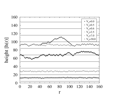
The intermittence implied by the result (15) is illustrated in Fig. 1 and in Fig. 2. As a function of , the manifold mostly stays almost unchanged in the current valley of minimum energy and occasionally jumps to another, new minimum of the periodic potential. A useful way to illustrate this intermittence as a function of is to calculate the configurational overlap between the ground states as a function of (in analogy with the overlap used in spin-glasses [13]). The overlap, is one if two configurations are the same and zero if they have no bonds in common. Fig. 2 presents the overlap as a function of amplitude of the pinning potential, , for interfaces in square and cubic lattices. The intermittent nature of periodic elastic media is clearly evident in these figures. Note that while the overlap and the interface roughness are intermittent, the interface energy (see Fig. 3) does not show any obvious signs of the jumps. Due to the logarithmic reduction in the gap size [Eq. (4)], the interface will only sample an infinitesimal fraction [] of the available minima of the potential as we sweep . Nevertheless a large number of different minima [] will be sampled by the system in particular if is increased while the transverse size is kept fixed.
IV Roughening of the Manifolds
The behavior of the roughness of interfaces seen in Fig. 3 is also strongly intermittent, especially in ()- dimensions. The large jumps in roughness seen in this figure are easily understood from the Imry-Ma arguments [14] concerning the instability of interfaces to large fluctuations, as we now demonstrate for the ()-dimensional case.
The interface energy of a subregion of the interface is, of course, also drawn from the Gaussian, , but now with standard deviation . Some of these energy fluctuations are favorable while others are unfavorable. The largest favorable fluctuations are found by setting , similarly to the extreme statistics arguments as in deriving Eq. (3), and it gives as the value of the energy gain,
| (16) |
A flat interface would like to take advantage of such large favorable energy fluctuations in adjacent minima of the periodic potential. However this requires having segments of the interface crossing the barriers in the periodic potential. We define the barrier cost per bond to be and this is given by the integral over the barrier, . We shall use the last of these forms as we shall often be interested in the dependence on . We consider and dimensional systems of wavelength , length and width , so that is the area of the part of the interface, which crosses the energy barrier, and in order to maximize the energy gain. is the two dimensional case, and in the isotropic three dimensional case. The barrier energy cost is given by
| (17) |
Equating Eqs. (16) and (17), yields the estimate of the parameter values at which the first “Imry-Ma” jump in the manifold roughness occurs,
| (18) |
In the ()-dimensional case the logarithmic correction drops out, by elementary considerations.
An “Imry-Ma” fluctuation of size leads to a jump in the roughness, which is of order , since . We emphasize that this is the expected outcome in any system with fixed disorder, when is varied. If , there is an exponential dependence of the crossover length on the parameters, for example, for ,
| (19) |
an exponential dependence on [14].
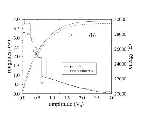
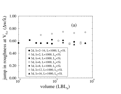
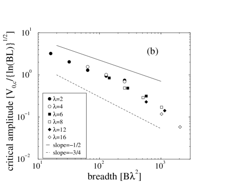
In Fig. 3, we present the numerically observed behavior of the interface roughness as a function of . We observe that for very large the interfaces are flat and are confined to a minimum of the potential. For a large range of the roughness stays the same or increases slowly (in three dimensions), until finally at a critical value a discrete jump occurs due to the “Imry-Ma” nucleation process. This implies that the roughening process, as defined by the point at which the interfaces begin to fluctuate outside a single valley, has a first-order character. It is seen from Fig. 4(a) that the first jump is as expected for an extensive fluctuation. The critical value at which the first extensive fluctuation occurs [Fig. 4(b)] follows roughly the prediction of Eq. (18) though the slope is closer to 3/4 instead of 2/3.
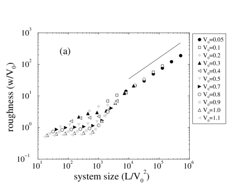
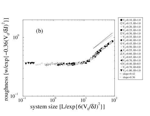
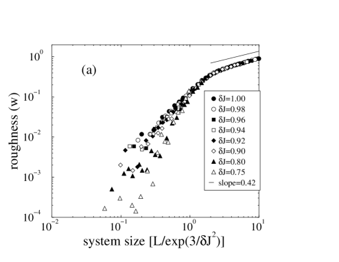
The analysis of the last paragraph clearly demonstrates that the roughening of manifolds in periodic elastic media is via a first order jump in roughness which is of order the wavelength of the periodic elastic medium. It is interesting to investigate whether this first order jump is observable in the ensemble averaged behavior. Scaled, ensemble-averaged plots of the manifold roughness as a function of are presented in Fig. 5 for {11} interfaces [Fig. 5(a)] and for {111} oriented interfaces [Fig. 5(b)]. These plots scale quite nicely with the characteristic length and roughness suggested by Eqs. (18) and (19). In the two dimensional case, there is also a clear indication of the first order character of the transition. The three dimensional data gives little indication of the first order jump in roughness and underscores the problems with a naive averaging of the data. However, we do not have any clear explanation, why the roughness values in the plateau before the jump can be collapsed with the same prefactor as in the asymptotic roughness in the {111} case, but not in the {11} case.
V Periodicity due to the Lattice
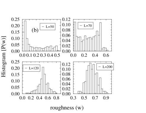
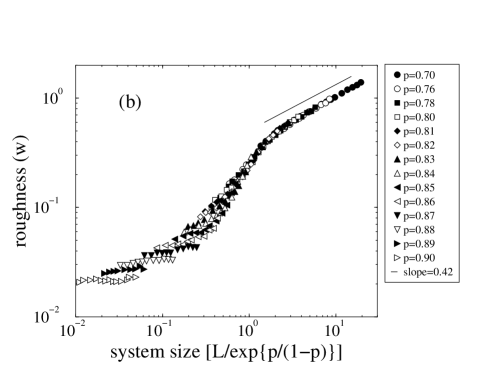
It is of interest to see if the first order character of the roughening of PEM extends to manifolds in the {10} and {100} directions. In these directions, the lattice itself introduces a periodicity, which for example is the origin of the thermal roughening transition in lattice models in three dimensions. Thus we do not need to introduce an extra periodic potential, and instead we just study the roughness of these manifolds as a function of disorder. We have studied the roughness of {100} manifolds as a function of disorder before and in those studies we ensemble averaged the data [15]. In the light of the understanding develop above, we have revisited this problem and find that the typical behavior in both the {10} and {100} problems is very similar to that suggested by the PEM model. That is, in a large sample the system roughens via a first order jump in the roughness due to an extensive fluctuation. The behavior of one sample as a function of disorder is presented in Fig. 6(a). The probability distributions of the roughness for several are presented in Fig. 6(b) in which we observe how one can pass through a co-existence region with both flat and rough samples as is varied. The intermittent behavior typical of PEM is evident in Fig. 6(a), but is obscured by the averaging in Fig. 7(a). Though the jump transition from the flat phase to the algebraically rough phase occurs in both the periodic elastic model in the {111} direction and for interfaces in the {100} direction, there is an important difference in the behavior of these models [compare Figs. 5(b) and 7(a)]. In the PEM model in the {111} direction, there is a pronounced plateau in the roughness due to the saturation of wandering within one well [Fig. 5(b)]. In contrast, in the {100} direction, the interface remains flat until the transition to the algebraically rough phase [see Fig. 7(a)]. The extent of the plateau region can be tuned in the PEM model by varying the shape of the potential near the minimum and by varying the wavelength. We have also carried out calculations for the case of dilution disorder [Fig. 7(b)] and find similar behavior, with the averaged behavior presented in Fig. 7(a). With dilution disorder the pronounced plateau is not due to any roughening inside a valley, but because of rare “bumps”, whose occurrence is due to the Poissonian statistics of diluted bonds. The averaged data scales quite well with , where and the variance of the binomial distribution with the corresponding mean , and is the occupation probability of a bond. Thus we find, in contrast to our earlier conclusions from similar data, that at large enough length scales interfaces in the {100} orientation are algebraically rough and are consistent with the PEM model.
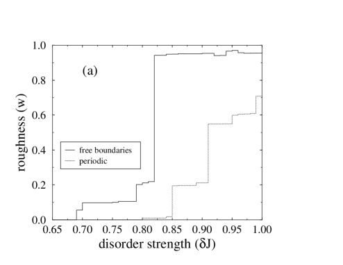
A further important feature of the large fluctuation character of the roughening transition is that it is strongly dependent on the boundary conditions. This is illustrated in Figs. 2(b) and 5(a) in which the roughness is depicted as a function of the amplitude of the disorder for both periodic and free boundaries and with the same disorder configuration. The threshold value of at which the first order jump in roughening occurs is typically smaller for the case of periodic boundaries. Large fluctuations can take advantage of the boundary to reduce the cost of crossing the energy barrier. This sensitivity to boundary conditions is a hallmark of the large fluctuation effects discussed here.
VI Conclusions
To conclude, we have discussed the roughening of elastic manifolds in the presence of a competition between bulk randomness and a confining periodic potential. We have concentrated on the two- and three-dimensional cases which are well-known to have, asymptotically, an algebraic roughness scaling. A study of the system-by-system behavior reveals however a much richer scenario in which each manifold makes intermittent jumps, finally culminating in a first-order change in its roughness. This process is also important since it is related to the asymptotic scaling of the roughness. Recent experiments on the creep of (1+1)-dimensional systems [2] have shown that scaling arguments of activation energy barriers can match real systems, using predictions based on rough manifolds. The time scales also depend crucially on the actual amplitude which is set in our picture by the roughening transition.
Also, the intermittence in the early stages would merit experimental consideration. Such jumps in the mean location of the interface, could be studied in the asymptotic rough regime. In an independent study we have pointed out this mechanism for both fracture surfaces arising from random fuse networks, and from yield surfaces of perfectly plastic media which are equivalent to the minimum energy surfaces studied here [16].
The focus of renormalization group and variational calculations in this problem has been dimensions , since there one encounters two asymptotic regimes separated by a transition. Of the two phenomena discussed here at least the intermittent jumps in the center of mass location of the interface should persist in that case.
Acknowledgements
This work has been supported by the Academy of Finland’s Centre of Excellence Programme (ETS and MJA). PMD thanks the DOE under contract DOE-FG02-090-ER45418 for support.
REFERENCES
- [1] T. Halpin-Healy and Y.-C. Zhang, Phys. Rep. 254, 215 (1995).
- [2] S. Lemerle, J. Ferré, C. Chappert, V. Mathet, T. Giamarchi, and P. Le Doussal, Phys. Rev. Lett. 80, 849 (1998); P. Chauve, T. Giamarchi, and P. Le Doussal, Phys. Rev. B 62, 6241 (2000). T. Nattermann, Y. Shapir, and I. Vilfan, Phys. Rev. B 42, 8577 (1990).
- [3] E. T. Seppälä, M. J. Alava, and P. M. Duxbury, Phys. Rev. E, 62, 3230 (2000).
- [4] J.-Ph. Bouchaud and A. Georges, Phys. Rev. Lett. 68, 3908 (1992); T. Emig and T. Nattermann Phys. Rev. Lett. 81, 1469 (1998); T. Emig and T. Nattermann, Eur. Phys. J. B 8 525, (1999).
- [5] D. Fisher, Phys. Rev. Lett. 56, 1964 (1986); A. A. Middleton, Phys. Rev. E 52, R3337 (1995).
- [6] A. J. Bray and M. A. Moore, Phys. Rev. Lett. 58, 57 (1987); G. Parisi, J. Phys. France 51, 1595 (1990). M. Mezard, J. Physique 51, 1831 (1990).
- [7] Y.-C. Zhang, Phys. Rev. Lett. 59, 2125 (1987); T. Nattermann, Phys. Rev. Lett. 60, 2701 (1988); M. V. Feigel’man and V. M. Vinokur, Phys. Rev. Lett. 61, 1139 (1988).
- [8] M. Alava, P. M. Duxbury, C. Moukarzel, and H. Rieger, in Phase Transitions and Critical Phenomena, edited by C. Domb and J. L. Lebowitz (Academic Press, San Diego, 2001), vol. 18.
- [9] A. V. Goldberg and R. E. Tarjan, J. Assoc. Comput. Mach. 35, 921 (1988).
- [10] J. Galambos, The Asymptotic Theory of Extreme Order Statistics, (John Wiley & Sons, New York, 1978); E. T. Seppälä, M. J. Alava, and P. M. Duxbury, submitted to Phys. Rev. E.
- [11] This idea is similar to what happens in the case of random manifolds in an external field, see E. T. Seppälä and M. J. Alava, Phys. Rev. Lett. 84, 3982 (2000).
- [12] This is analogous to wetting in random systems, see R. Lipowsky and M. E. Fisher, Phys. Rev. Lett. 56, 472 (1986).
- [13] Spin Glasses and Random Fields, edited by A. P. Young, (World Scientific, Singapore, 1997).
- [14] Y. Imry and S.-k. Ma, Phys. Rev. Lett. 35, 1399 (1975); K. Binder, Z. Phys. B 50, 343 (1983); also the similar arguments in [4].
- [15] M. J. Alava and P.M. Duxbury, Phys. Rev. B 54, 14990 (1996); see also V. I. Räisänen, E. T. Seppälä, M. J. Alava, and P. M. Duxbury, Phys. Rev. Lett. 80, 329 (1998).
- [16] E. T. Seppälä, V. I. Räisänen, and M. J. Alava, Phys. Rev. E 61, 6312 (2000).