Distribution of sizes of erased loops of loop-erased random walks in
two and three dimensions

Abstract

We show that in the loop-erased random walk problem, the exponent characterizing probability distribution of areas of erased loops is superuniversal. In $d$-dimensions, the probability that the erased loop has an area $A$ varies as $A^{-2}$ for large $A$, independent of $d$, for $2\leq d\leq 4$. We estimate the exponents characterizing the distribution of perimeters and areas of erased loops in $d=2$ and $3$ by large-scale Monte Carlo simulations. Our estimate of the fractal dimension $z$ in two-dimensions is consistent with the known exact value $5/4$. In three-dimensions, we get $z=1.6183\pm 0.0004$. The exponent for the distribution of durations of avalanche in the three-dimensional abelian sandpile model is determined from this by using scaling relations.

I Introduction

The loop erased random walk (LERW) problem was first defined by Lawler [3] as a more tractable variant of the well-known self-avoiding walk problem. The problem turns out to be related to many well-studied problems in statistical physics, but seems to have attracted less attention than it deserves. It was shown by Lawler [4] to be equivalent to a special case of the Laplacian self-avoiding walk problem defined by Lyklema et al. [5]. Majumdar [6] showed that this model is equivalent to the classical graph-theoretical problem of spanning trees on graphs, and the $q$-state Potts model in the limit $q\to 0$. This equivalence also makes this problem related to the abelian sandpile model of self-organized criticality [7]. In fact, as we shall show in this paper, this model provides a numerically efficient method of determining the only unknown critical exponent of the abelian sandpile model in three-dimensions.

This prompted us to undertake the numerical study of the LERW’s in $d=2$ and $3$ reported in this paper. We obtain fairly precise estimates of the fractal dimension of LERWs in $d=2$ and $3$. We note the interesting consequence of the scaling theory that the distribution of the area of the erased loop has the same exponent $2$, independent of the dimension $d$, for $2\leq d\leq 4$. In $d=3$, the numerical value of fractal dimension of LERW’s enables us to determine the avalanche durations exponent of the abelian sandpile model, using the scaling relations and other exactly known exponents of the model [8].

A good review of earlier results on the LERW problem can be found in [9]. Lawler showed that the fractal dimension $z$ of LERWs is $2$ for $d\geq 4$, and $z\leq(d+2)/3$ for $d\leq 4$ [9]. Recently, it was shown rigorously that in two-dimensions $z$ is strictly larger than 1 [10]. Using the known exact results about the critical exponents of Potts model from conformal field theory, Majumdar was able to prove exactly that $z=5/4$ for LERW problem in $d=2$ [6], a result which was guessed earlier by Guttmann and Bursill from numerical simulations [11]. A proof of this result without using conformal field theory has been given by Kenyon [12]. Using conformal invariance, Duplantier has obtained the exact probabilities of no intersection of $n$ LERWs of $\ell$ steps starting near each other in two-dimensions, and also the winding angle distribution [13]. The distribution of sizes of erased loops was first studied in [14]. Priezzhev has used bounds on intersection probability of loop erased walks with random walks to show that the upper-critical dimension of the Bak-Tang-Wiesenfeld (BTW) sandpile model is 4 [15].

The plan of this paper is as follows: The LERW model is defined in Sec. II. In Sec. III, we recall the main points of the scaling theory of the distribution of erased loops [14], and apply it to show that the exponent characterizing the distribution of area enclosed by erased loop is the same for $2\leq d\leq 4$. We determine the behavior of the distribution functions for the perimeter and the area of the loop in the scaling limit, for very small or very large values of the argument of the scaling functions. The simulation technique and the results obtained are described in Sec. IV. The exponent characterizing the distribution of durations of avalanches in BTW sandpile model in $d=3$ is determined in Sec. V, and some concluding remarks follow in Sec. VI.

II Definition of the Model

Consider a simple random walk on a $d$-dimensional lattice. We start with a particular realization ${\cal W}$ of the random walk having $N$ steps, ${\cal W}=\{w_{0}$, $w_{1}$, $w_{2}$, $\ldots$, $w_{N-1}$, $w_{N}\}$, where $w_{i}$ is the site reached by the $i$-th step of walk. We define the LERW ${\cal L}$ corresponding to ${\cal W}$ as the path obtained from ${\cal W}$ by erasing each loop as soon as it is formed. If ${\cal W}$ has no self-intersections, we define ${\cal L}={\cal W}$. If ${\cal W}$ has self-intersections, let $j$ be earliest step which leads to self-intersection in ${\cal W}$, so that $j$ is the least integer such that $w_{j}=w_{i}$ for some $i<j$. Then, we obtain a new walk ${\cal W}^{\prime}=\{w_{0}$, $w_{1}$, $\ldots$, $w_{i}$, $w_{j-1}$, $\ldots$, $w_{N-1}$, $w_{N}\}$ by deleting all steps between $i$ and $j$, keeping $i$ and deleting $j$. This process, corresponding to loop erasure of the earliest loop formed, is repeated till loops can no longer be found. The resulting walk ${\cal L}$ is the required LERW corresponding to ${\cal W}$. This procedure of loop-erasure is illustrated in Fig. 1.

The length of ${\cal L}$ is the number of steps in ${\cal L}$. We will denote it by $n$. For a fixed $N$, $n$ is a random variable. We define the critical exponent $z$ of the LERW by the relation that

$$\langle n\rangle\sim N^{z/2}$$ (1)

for large $N$, where the angular brackets denote averaging over all random walks of $N$ steps. As the root-mean-square end to end distance $R$ is same as for random walks, we have $R\sim N^{1/2}$, and $\langle n\rangle\sim R^{z}$. Thus, $z$ is the fractal dimension of the LERW.

III Scaling Theory for the Distribution of Loop-sizes

Let $\text{Prob}(\ell,N)$ denote the probability that a loop of perimeter $\ell$ will be erased at the $N$-th step of the random walk. Let $F(\ell,N)$ denote the cumulative probability that a loop of perimeter $\ell$ or greater will be erased at the $N$-th step of the random walk. We shall study the behavior of this function for large $N$, and write

$$\text{Prob}(\ell)=\lim_{N\to\infty}\text{Prob}(\ell,N)$$ (2)

and

$$F(\ell)=\lim_{N\to\infty}F(\ell,N)$$ (3)

We adopt the convention that if no loop is formed at a step, it will be said to be erasure of loop of perimeter $0$. With this convention, we clearly have $F(0,N)=1$, for all $N$.

For $d\leq 4$, the mean number of loop-length erased per step tends to $1$ for large $N$. This implies that

$$\sum_{\ell=0}^{\infty}\ell\text{~{}Prob}(\ell)=1,\quad\text{for~{}}d\leq 4$$ (4)

For large $\ell$, $F(\ell)$ is expected to vary as a power of $\ell$, say as $\ell^{-\tau+1}$. However, for a finite $N$, there is a cutoff size $\ell^{\star}$, and loops of size $\ell>\ell^{\star}$ are very unlikely. The cutoff value $\ell^{\star}$ varies as a power of $N$, say $\ell^{\star}\sim N^{\phi}$. This suggests that $F(\ell,N)$ satisfies the scaling form

$$F(\ell,N)\sim\ell^{-\tau+1}f\bigl{(}\ell/N^{\phi}\bigr{)}$$ (5)

The cutoff exponent $\phi$ can be determined by the following simple argument [14]: The cutoff for the perimeter of erased loops should also vary as $\langle n\rangle$, the average length of the LERW after $N$ steps. Since this scales as $N^{z/2}$ [Eq. (1)], we get $\phi=z/2$.

The exponent $\tau$ is also expressible in terms of $z$. For $\ell\ll\ell^{\star}$, the total number of loops of size $\geq\ell$ for a walk of $N$ steps varies as $NF(\ell)$, and is much greater than $1$. For $\ell>\ell^{\star}$, we expect a much stronger decay. For $2\leq d\leq 4$, we get a significant number of large loops, and thus in this case, we expect that

$$NF(\ell^{\star},N)\sim O(1)$$ (6)

Putting in the scaling form (5), this implies that

$$\tau=1+2/z$$ (7)

Thus, the scaling form for the distribution of loop perimeters is determined in terms of a single exponent $z$, and is given by

$$F(\ell,N)\sim\ell^{-2/z}f\bigl{(}\ell/N^{z/2}\bigr{)},\quad\text{for~{}}\ell\gg 1.$$ (8)

The scaling function $f(x)$ is assumed to tend to $1$ as $x$ tends to zero, and tend to zero for large $x$. We define

$$\Delta\text{Prob}(\ell,N)=\text{Prob}(\ell,N)-\text{Prob}(\ell)$$ (9)

If for $x$ near zero, $1-f(x)$ varies as $x^{a}$, we see that keeping $\ell$ fixed, and in the limit of large $N$

$$\Delta\text{Prob}(\ell,N)\sim-K_{\ell}N^{-az/2}$$ (10)

where $K_{\ell}$ is an $\ell$-dependent constant, and the exponent is independent of $\ell$. It is easy to calculate $\text{Prob}(2,N)$ in arbitrary dimension $d$. The conditional probability of forming a loop of perimeter $2$ at the $N$-th step is $0$, if the random walker returned to origin at step $(N-1)$, and it is $1/(2d)$ otherwise (for a $d$-dimensional hypercubical lattice with coordination number $2d$). Thus

$$\text{Prob}(2,N)=\frac{1}{2d}(1-g_{N})$$ (11)

where $g_{N}$ is the probability that the random walker returns to origin after $N-1$ steps. In $d$-dimensions, $g_{N}$ varies as $N^{-d/2}$ for large $N$. Thus, we see that for large $N$, $\Delta\text{Prob}(2,N)$ varies as $N^{-d/2}$. Comparing this with Eq. (10), we see that $a=d/z$. Thus, we get

$$f(x)\simeq 1-Kx^{d/z},\quad\text{for~{}}x\text{~{}near~{}}0.$$ (12)

[We shall denote an undetermined constant by $K$. Its value in different equations need not be the same.] For other values of $\ell\neq 2$, this then implies that

$$K_{\ell}\simeq K\ell^{d/z},\quad\text{for~{}}\ell\gg 1.$$ (13)

This may be understood as follows: The main deviation of $\text{Prob}(\ell,N)$ from its asymptotic value comes from the cases when the LERW at step $N-1$ is of length $\lesssim\ell$, and the probability that walker after $N$ steps is within a sphere of radius $\ell^{1/z}$ centered at the origin varies as $\ell^{d/z}N^{-d/2}$ for $\ell\ll N$.

We can also determine the leading $N$-dependence of $\text{Prob}(\ell=0,N)$. Since for any non-zero $\ell$, $\text{Prob}(\ell,N)$ is less than than its limiting value for large $N$, $\text{Prob}(0,N)$ must be larger than $\text{Prob}(0)$. In fact

$$\Delta\text{Prob}(0,N) = -\sum_{\ell=2}^{\infty}\Delta\text{Prob}(\ell,N)$$ (14)

$$\sim KN^{-d/2}\sum_{\ell}\ell^{(d-2-z)/z}$$ (15)

This summation over $\ell$ has an upper cutoff proportional to $\ell^{\star}$. In two dimensions, we get

$$\Delta\text{Prob}(\ell=0,N)\sim K(\log N)/N$$ (16)

In three dimensions, the summation diverges as $(\ell^{\star})^{1/z}\sim N^{1/2}$. Thus, we get

$$\Delta\text{Prob}(\ell=0,N)\sim K/N,\quad\text{for~{}}d=3.$$ (17)

For large $x$, $f(x)$ is expected to decrease as $\exp(-Kx^{b})$. The exponent $b$ can be determined as follows: We note that for any constant $\epsilon\ll 1$, the probability that a loop of perimeter $\epsilon N$ is formed at $N$-th step should vary as $\exp\{-K(\epsilon)N\}$ for fixed $\epsilon$ and $N$ tending to infinity [17]. This implies that $b=2/(2-z)$, and hence

$$f(x)\sim\exp\Bigl{(}-Kx^{2/(2-z)}\Bigr{)},\quad\text{for large~{}}x.$$ (18)

An interesting quantity is the area enclosed by a loop. In two-dimensions, this is straightforward to determine. In three-dimensions, it may be defined as the minimum number of plaquettes required to form a simply-connected surface bounded by the loop. In this study, we used an alternate, computationally simpler, measure of this area. We simply project the loop on to the three coordinate planes, and measure the areas of the projections. If the three areas are $a_{1}$, $a_{2}$ and $a_{3}$, we define the area of the loop to be $(a_{1}^{2}+a_{2}^{2}+a_{3}^{2})^{1/2}$. The generalization to higher dimensions is obvious.

Let $F(A,N)$ be the probability that a loop of area greater than or equal to $A$ generated at the $N$-th step of the random walk. A loop of perimeter $\ell$ has a linear size $R\sim\ell^{1/z}$ and an area $A\sim R^{2}$, then, it is easy to see from Eq. (8) that for $N,A\gg 1$

$$F(A,N)\sim A^{-1}g(A/N)$$ (19)

Here also the scaling function $g(x)$ goes to a constant for $x\to 0$, and decreases rapidly to zero for $x\gg 1$.

Thus we find the rather unexpected result that the distribution for the area of the loop is independent even of $z$, and hence is the same for all dimensions $d$, with $2\leq d\leq 4$. This argument does not work in $d=1$, as there $\text{Prob}(\ell)$ decreases exponentially with $\ell$, and the scaling theory assuming power-law decays fails [16]. For $d\geq 4$, the LERW behaves as a random walk, and for random walks, the area of loop varies as the perimeter of the loop. Hence we would expect that the probability that a loop of area $A$ is formed varies as $A^{-d/2}$ for $d>4$. The probability that a loop of area greater than or equal to $A$ is formed, varies as $A^{-d/2+1}$ for $d>4$.

Using the fact that $A$ varies as $\ell^{2/z}$ for $\ell\lesssim\ell^{\star}$, from Eq. (12) we see that the function $g(x)$ determining the finite-$N$ cutoff effects varies as

$$g(x)\simeq g(0)\exp\bigl{(}-Kx^{d/2}\bigr{)},\quad\text{for small~{}}x.$$ (20)

For large $x$, $g(x)$ should vary as $\exp(-Kx^{c})$, where $c$ is some exponent. Let $\epsilon$ be a small number $\ll 1$. Using the fact that loops of area $\epsilon L^{2}$ should decrease only as $\exp\{-K(\epsilon)L\}$ for fixed $\epsilon$ in the limit of large $L$, we see that $c=1$, and

$$g(x)\sim\exp(-Kx),\quad\text{for large~{}}x.$$ (21)

It is interesting to compare this behavior with that of $f(x)$ for large $x$. These behaviors are consistent only if for a large loop of area $A\gg N$, the average perimeter varies as

$$\ell\sim\ell^{\star}(A/N)^{1-z/2}$$ (22)

This behavior should be contrasted with the behavior for $A\ll N$, where the average perimeter varies as $A^{z/2}$ with no explicit dependence on $\ell^{\star}$. It is interesting to note that this scaling law for large loops remains valid even outside the scaling limit for $A$ of order $N^{\alpha}$ with $1\leq\alpha\leq 2$. For $\alpha=2$, it gives perimeter proportional to $N$, as it should.

IV Numerical Simulations

The simplest algorithm to simulate the LERW problem on computer is to actually generate the trail of a random walk step-by-step on a $d$-dimensional lattice. At each new step, if a loop is formed it is erased. This is straight-forward to implement, but requires large memory in large dimensions $d$, as for simulating a walk of $N$ steps, one needs to have a lattice of linear size $N^{1/2}$, which means that the required memory increases as ${\cal O}\bigl{(}N^{d/2}\bigr{)}$.

The algorithm that makes the most efficient use of memory would store the walk as a linked list, keeping only the unerased steps. But there is a memory/CPU tradeoff, and the computation time increases as searching for self-intersections is very inefficient in this scheme.

In our simulations we used a hybrid scheme for storing the coordinates of the points visited by the walk. We store the coordinates of the LERW in not one, but $M$ lists, where $M$ is a large number. There is a unique hashing rule which assigns a site to one of the lists, so that checking for intersection has to be done only within one list. To see if a point already belongs to the LERW, we have to search only in the list corresponding to the point in question. The best choice of $M$ is ${\cal O}(\ell^{\star})$, as then each list has ${\cal O}(1)$ entries. With this, we were able to simulate a two-dimensional walk of $2^{33}$ steps in about 3 hours 16 minutes using $\sim 60$ Mb of memory on a 350 MHz Pentium-II machine. In three-dimensions, a walk of $2^{29}$ steps took about $24$ minutes and $\sim 300$ Mb of memory on a similar machine.

Simulations were carried out for total walk length $N$ of $2^{r}$ steps, with $r=25,\ldots,29$ for two-dimensional walks and $r=24,\ldots,28$ for three-dimensional walks. To eliminate the initial transients, we collected the statistics of loops only after discarding the first $N/2$ steps. In addition, ensemble average was taken over $10^{3}$ distinct realizations of random walks in each case. For the two-dimensional case we also simulated a small number of walks for $r$ up to $34$.

A Two-dimensional LERW

In Fig. 2 we show the plot for the cumulative distribution function $F(\ell,N)$ [18]. We plot $\ell^{2/z}F(\ell,N)$ versus $\ell$. There is a significant deviation from simple power-law behavior for very small $\ell$, and for large $\ell$. For $\ell\lesssim\ell^{\star}$, the data fits well to the functional form given by Eq. (12). In the small $\ell$ regime, the leading correction is a correction to scaling. Incorporating this, we fit the data to the form

$$F_{0}(\ell,N)=\frac{C_{1}}{\ell^{C_{2}}}\exp\left[-C_{3}\bigl{(}\ell^{C_{2}}/N\bigr{)}^{-d/2}\right]\left(1+\frac{C_{4}}{\ell^{C_{5}}}\right)$$ (23)

where $C_{2}$ is related to the fractal dimension via $C_{2}=2/z$.

The best fit values of all the parameters in Eq. (23) are tabulated in Table I. We note that $C_{5}$ is $1$ within our error bars. Furthermore, the exact value of $C_{2}$ is also known to be $8/5$. As a result, one more set of values were estimated for the parameters by constraining $C_{2}$ and $C_{5}$ to these values. The parameter values thus obtained are also tabulated in Table I. The fit is rather good for all $\ell\gtrsim 10$. Statistical fluctuations are large for $\ell\gtrsim 10^{4}$, as there are not many such loops generated.

In Fig. 3 we have plotted the $AF(A,N)$ versus $A$ for different values of $N$, and also shown the best fit using the fitting form Eq. (23) with $\ell$ substituted by $A$. While estimating the parameters we constrained $C_{2}$ and $C_{5}$ to $1$. This is because the exact value of $C_{2}$ is known to be $1$ and unconstrained value of $C_{5}$ turns out to be $1$ within error bars. This allows a better estimate of the remaining parameters. The estimated best fit values of parameters for this data set are tabulated in Table I. It is clearly seen from Fig. 3 that the scaling form fits the data very well in nearly the entire range.

We obtained more accurate estimates of $\text{Prob}(\ell,N)$ for $\ell\leq 100$ by taking an ensemble average over $10^{9}$ different realizations of the random walk. In Fig. 4, we have plotted the variation of $N\Delta\text{Prob}(\ell,N)$ versus $\log(N)$ in two dimensions for $\ell=0$, $2$, $4$ and $6$. We see clearly that while $N\Delta\text{Prob}(0,N)$ has a linear variation with $\log(N)$, for other values of $\ell$, this tends to a limiting constant value for $\ell\gg 1$.

B Three-dimensional LERW

The distribution of loop-sizes for the three-dimensional walks by perimeter is shown in Fig. 5. The format of presentation is exactly the same as in the previous subsection. We fit the data to the form given by Eq. (23). From the figure it is seen that this scaling form fits the entire data very well for $\ell\gtrsim 10$. The best fit values of parameters in this equation are tabulated in Table I. We find that in this case the best-fit value of the correction to scaling exponent $C_{5}$ turns out to be $0.86$, clearly different from $1$.

Our estimate of the best fit value of the fractal dimension $z$ gives

$$z=1.6183\pm 0.0004,\qquad d=3$$ (24)

This value is not very sensitive to the choice of parameters $C_{1}$, $C_{3}$, $C_{4}$, and $C_{5}$. The error bar on $z$ gives our subjective estimate of errors of extrapolation. This should be compared with the value $z=1.623\pm 0.011$ obtained by Guttmann and Bursill [11]. Because of the larger fractal dimension of walks, for the same value of $N$, there are significantly more longer loops generated in $d=3$ than in $d=2$. As a result, we see power-law scaling over roughly $5$ decades of $\ell$ in Fig. 5 compared to that of about $4$ decades of $\ell$ in Fig. 2.

In Fig. 6 we show the plot for $F(A,N)$ the cumulative distribution function for loop area. We have plotted $AF(A,N)$ versus $A$ for different values of $N$. An unbiased estimate of $C_{2}$ from the best-fit gives a value $1.00000\pm 0.00005$. Thus, we put $C_{2}$ to be exactly $1$ and estimated the remaining parameters by fitting the scaling form given by Eq. (23) with $\ell$ substituted by $A$. From the figure it is clearly seen that this form approximates the entire data very well for $A\gtrsim 10$. The estimated values of parameters is tabulated in Table I. Here also, the exponent in the correction to scaling term turn out to be different from $1$.

In Fig. 7 we have replotted the data of Fig. 6 with $AF(A,N)$ plotted against $(A/N)^{3/2}$. We see that the curves are approximately linear for small $A/N$, verifying the theoretical prediction of Eq. 20. For larger values of $A/N$, the slope decreases as expected from Eq. 21.

In Fig. 8, we have plotted the variation of $\Delta\text{Prob}(\ell,N)$ versus $N$ for $\ell=0$, $2$, and $4$. The data was obtained by averaging over $10^{9}$ different realizations of $100$-stepped walks. For $\text{Prob}(\ell)$, we used the values from the $N=2^{28}$ simulation. We see good agreement with the predicted $1/N$ variation for $\ell=0$, and $1/N^{3/2}$ variation for $\ell=2$ and $4$.

V Relation to Exponents of the Sandpile Model

The sandpile model of Bak-Tang-Wiesenfeld is defined as follows [19]: We consider a hypercubical lattice of linear size $L$ in $d$ dimensions. At each site is a non-negative integer which gives the “height” of the pile at that point. The system is driven by adding a grain of sand at a randomly chosen site, thereby increasing the height of pile at that site by one. If the height at any site exceeds $(2d-1)$, it topples, and its height decreases by $2d$, and one grain is transferred to each of its neighbors. If this makes some other sites unstable, they are toppled in turn, until all sites are stable, and then a new grain of sand is added.

Bak et al. observed that in the steady state of such a pile, adding a grain gives rise to a sequence of topplings, and the size of such avalanches is a random variable with a power-law tail. Determining the exact values of the exponents characterizing these tails has been the main theoretical problem in the area of self-organized criticality.

The model in $d=1$ is rather trivial, and does not show simple power-law tails of avalanche sizes, as most avalanches are large [20]. In $d=2$, unlike in $d=1$, most avalanches are finite, but they involve multiple topplings of sites. A theoretical understanding of this case remains incomplete [21]. For $d\geq 4$, mean-field description of avalanche propagation is adequate, and the corresponding exponents are the same as of sizes of clusters in critical percolation theory [15].

The BTW model for $d=3$ does not suffer from the problems caused by multiple topplings. It is thus the simplest undirected model for studying self-organized criticality with nontrivial (non-mean-field) critical behavior. In this case, multiple topplings at a site occur with very low probability, and the avalanche clusters are found to be compact, with fractal dimension $3$. Then, simple scaling arguments [22, 8] show that if the probability that there are exactly $s$ topplings in an avalanche in a system of linear size $L$ is $\text{Prob}(s\mid L)$, which satisfies the simple finite-size scaling form

$$\text{Prob}(s\mid L)\sim s^{-a}h\bigl{(}s/L^{b}\bigr{)}$$ (25)

then we must have $a=4/3$ and $b=3$.

The theoretical assumptions that go into the scaling argument have been checked extensively in simulations, but a rigorous theoretical proof is not yet available. Since the number of distinct toppled sites is assumed to be proportional to the number of topplings, we see that the probability that an avalanche has $s_{d}$ distinct sites toppled also varies as $s_{d}^{-4/3}$.

As a check on the scaling theory, note that the probability that avalanche reaches a distance $R$ scales as the probability that number of topplings is greater than $R^{3}$, hence as $1/R$, which also agrees with the known result about expected number of topplings at a distance $R$.

The only exponent which this simple argument does not give is the exponent for the duration of avalanches. But the propagation of avalanches occurs along spanning trees path in the equivalence between the sandpile model and spanning trees [7]. Hence, the duration $T$ of an avalanche must vary with its linear extent as $T\sim R^{z}$. And the $z$ is for spanning trees, which is the same as the $z$ we used for LERWs. The knowledge of $z$, thus, allows us to estimate the exponent for duration of avalanches: the probability that the duration of avalanche is greater than $T$ varies as $T^{-y}$, where

$$y=1/z=0.61795\pm 0.00015$$ (26)

VI Concluding Remarks

We have already noted that the LERW problem is very suited for numerical studies. In the two-dimensional case, we have collected data for over $10^{3}$ realizations of walks with $N$ up to $2^{29}$. Thus the numerically determined loop-size distribution is an average over more than $8\times 10^{10}$ loops (only about $31.25\%$ of the steps taken form non-trivial loops on square lattice). For the three-dimensional case, the corresponding number is $2.8\times 10^{10}$ loops (only about $21.17\%$ steps form non-trivial loops on cubic lattice). The quantity which corresponds closest to loop-erasures are avalanches in the sandpile model (more correctly, subavalanches) [23]. Clearly, simulation of the Abelian sandpile model with equal number of avalanches is not possible with available computing machines.

Secondly, our simulations are done on an effectively infinite lattice, and there are no complicated boundary effects to complicate the analysis of data. Corrections due to finite size of system show up only in the finiteness of the number of steps $N$ of the random walk. This seems to be well described by simple finite-size scaling theory. If we wanted to determine the exponent $z$ using the sandpile model, or the spanning trees, the largest system sizes accessible would be much smaller.

The dimension-independence of the exponent characterizing the distribution of areas of erased loops for $2\leq d\leq 4$ is rather unexpected. The exponent does depend on dimension for $d>4$. We have been unable to find a more transparent proof of this result.

We would like to thank S. N. Majumdar for his critical reading of an earlier version of this paper.

TABLE I.: Estimated values of various parameters corresponding to Eq. (23) for variation of loop perimeter and area for two- and three-dimensional LERWs. The values without error bars are fixed during estimation of other parameters.

		$C_{1}$	$C_{2}$	$C_{3}$	$C_{4}$	$C_{5}$
2-D	$\ell$	$0.3533\pm 0.0004$	$1.5997\pm 0.0005$	$1.1\pm 0.1$	$1.58\pm 0.03$	$1.000\pm 0.007$
	$\ell$	$0.35385\pm 0.00025$	$8/5$	$1.1\pm 0.1$	$1.56\pm 0.03$	$1$
	$A$	$0.127316\pm 0.000015$	$1$	$9.8\pm 0.7$	$0.494\pm 0.003$	$1$
3-D	$\ell$	$0.1527\pm 0.0003$	$1.2359\pm 0.0003$	$2.8\pm 0.3$	$1.69\pm 0.02$	$0.86\pm 0.05$
	$A$	$0.1312\pm 0.0002$	$1$	$35\pm 7$	$0.142\pm 0.005$	$0.394\pm 0.015$

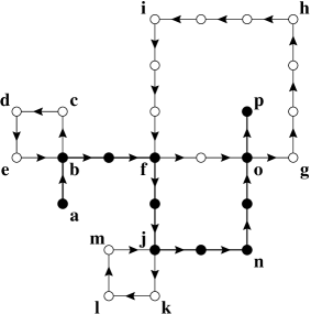
FIG. 1.: An illustrative example of the loop-erasing procedure: The random walk a-b-c-d-e-$\cdots$-p starts at a, and ends at p. The erased loops are shown by thin lines. Note that at the point o, while the random walk path intersects itself, the LERW encounters no intersection, as the loop f-g-h-i-f has already been erased.

FIG. 2.: Variation of $\ell^{2/z}F(\ell,N)$ with $\ell$ for two-dimensional LERW. Solid lines represent the best fit of Eq. (23) with parameter values (including estimate of $z$) given in Table I.

FIG. 3.: Variation of $AF(A,N)$ with $A$ for two-dimensional LERW. Solid lines represent the best fit of Eq. (23) with parameter values given in Table I.

FIG. 4.: Variation of $N\Delta\text{Prob}(\ell,N)$ with $N$ for $\ell=0$, $2$, $4$ and $6$ in two dimensions. For better visibility, the data points for $\ell=2$, $4$, and $6$ have been displaced vertically by $0.69$, $0.59$, and $0.57$ respectively.

FIG. 5.: Variation of $\ell^{2/z}F(\ell,N)$ with $\ell$ for three-dimensional LERW. Solid lines represent the best fit of Eq. (23) with parameter values given in Table I.

FIG. 6.: Variation of $AF(A,N)$ with $A$ for three-dimensional LERW. Solid lines represent the best fit of Eq. (23) with parameter values given in Table I.

FIG. 7.: Variation of $AF(A,N)$ with $100(A/N)^{3/2}$ for threedimensional LERW showing the behavior of the exponential correction term. Thick straight line represents the best fit of Eq. (23) with parameter values given in Table I.

FIG. 8.: Variation of $\Delta\text{Prob}(\ell,N)$ with $N$ for $\ell=0$, $2$, and $4$ in three dimensions. Straight lines show the fits using slopes $-1$ for $\ell=0$ and $-3/2$ for $\ell=2$ and $4$.

REFERENCES

- [1] E-Mail: himanshu@theory.tifr.res.in
- [2] E-Mail: ddhar@theory.tifr.res.in
- [3] G. F. Lawler, Duke Math J. 47, 655 (1980).
- [4] G. F. Lawler, J. Phys. A 20, 4565 (1987).
- [5] J. W. Lyklema and C. Evertz, J. Phys. A 19, L895 (1986). LERWs correspond to the parameter value of the general model defined here.
- [6] S. N. Majumdar, Phys. Rev. Lett. 68, 2329 (1992).
- [7] For a recent review, see D. Dhar, Physica A 263, 4 (1999); a longer review is available in the LANL archive [cond-mat/9909009].
- [8] D. V. Ktitarev, S. Lübeck, P. Grassberger and V. B. Priezzhev, Phys. Rev. E 61, 81 (2000).
- [9] G. F. Lawler, Intersections of Random Walks, (Birkhauser, Boston, 1991), Chap. 7.
- [10] G. F. Lawler, preprint math/9803034.
- [11] A. J. Guttmann and R. J. Bursill, J. Stat. Phys. 59, 1 (1990).
- [12] R. Kenyon, preprint (1999).
- [13] B. Duplantier, Physica A 191, 516 (1992).
- [14] A. Dhar and D. Dhar, Phys. Rev. E 55, R2093 (1997).
- [15] V. B. Priezzhev, J. Stat. Phys.,98 (2000) 667..
- [16] On a linear chain, only possible loops are of length zero or two. Longer loops do occur on more complicated one-dimensional graphs, such as ladders.
- [17] A similar argument, in the context of self-avoiding walks was used earlier in M. E. Fisher, J. Chem. Phys.,44 616 (1966).
- [18] To be precise, the function plotted is an average of with lying between and .
- [19] Bak P., Tang C. and Wiesenfeld K., Phys. Rev. Lett., 59 (1987) 381.
- [20] Ruelle P. and Sen S., J. Phys. A 25 (1992) 1257; Ali A. A. and Dhar D., Phys. Rev. E 51 (1995) R 2705.
- [21] Priezzhev V. B., Ktitarev D. V. and Ivashkevich E. V., Phys. Rev. Lett. 76 (1996) 2093; Paczuski M. and Boettcher S., Phys. Rev. E 56 (1997) R3745; De Menech M., Stella A. L., and Tebaldi C., Phys. Rev. E 58 (1998) R 2677.
- [22] Zhang Y. C., Phys. Rev. Lett., 63 (1989) 470.
- [23] Shcherbakov R. R., Papoyan V. V., and Povolotsky A. M., Phys. Rev E 55 (1997) 3686.