[

Transport through quasi-ballistic quantum wires: the role of contacts

Abstract

We model one-dimensional transport through each open channel of a quantum wire by a Luttinger liquid with three different interaction parameters for the leads, the contact regions and the wire, and with two barriers at the contacts. We show that this model explains several features of recent experiments, such as the flat conductance plateaux observed even at finite temperatures and for different lengths, and universal conductance corrections in different channels. We discuss the possibility of seeing resonance-like structures of a fully open channel at very low temperatures.

]

Recent advances in the fabrication of quantum wires within GaAs-AlGaAs heterostructures have made it possible to study their electronic transport properties in great detail [1, 2, 3, 4, 5, 6, 7, 8]. These studies show some puzzling features for the conductance of quantum wires; specifically, the flat conductance plateaux lying below integer multiples of $g_{0}\equiv 2e^{2}/h$ [1, 3, 4, 7, 8]. At the same time, the theory of Tomonaga-Luttinger liquids (TLL) has led to a general framework for understanding the effects of impurities and finite temperature and wire length on the conductance of strongly correlated electron systems in one dimension [9, 10, 11, 12, 13]. In this Letter, we propose a model for a quantum wire (QW) based on TLL theory which provides a unified way of understanding a large class of experiments including the features mentioned above.

Our model of a QW is motivated partly by the way these structures are fabricated and partly by the experimental observations. The electrons are first confined to a two-dimensional region which is the inversion layer of a GaAs heterostructure. Within that layer, a gate voltage $V_{G}$ is applied in a small region which further confines the electrons to a narrow constriction called the QW; this is typically a few microns long [1, 3, 4]. Within the QW, the electrons feel a transverse confinement potential produced by $V_{G}$; this leads to the formation of discrete subbands or channels. As argued in Ref. [14], the electrons from the two-dimensional electron gas (2DEG) can enter or leave a one-dimensional system like a wire only if they are in a zero angular momentum state with respect to the appropriate end of the wire. Since the radial coordinate is the only variable appearing in the wave function of such a state, the 2DEG electrons which contribute to the conductance may be modeled as one-dimensional noninteracting Fermi liquid systems lying on the two sides of the QW [10]; we will refer to these two semi-infinite systems as the leads. However when the electrons enter the constriction, they interact via the Coulomb repulsion. If the Coulomb repulsion is approximated by a short range interaction, the electrons in the wire can be described by a TLL. In fact, each open channel (defined below) can be modeled by a separate TLL. In addition, the charge and spin degrees of freedom are governed by independent TLL’s if the interactions are invariant under spin rotations and there is no magnetic field.

The simplest model which incorporates all these features is a one-dimensional system in which the TLL parameters (an interaction parameter $K$ and the quasiparticle velocity $v$) are functions of the coordinate $x$ as follows. If the QW lies in the range $0<x<l$, we let $(K,v)$ take the values $(K_{L},v_{L})$ for $x<0$ and $x>l$ (the leads), and the values $(K_{W},v_{W})$ for $0<x<l$ [10, 11]. (The parameters $K_{W}$ and $v_{W}$ will also carry charge and spin labels $\rho$ and $\sigma$; we will include these later). Here $v_{L}$ is equal to the Fermi velocity $v_{F}={\sqrt{2E_{F2D}/m}}$ of the electrons in the 2DEG (thus $v_{L}$ depends on the density and effective mass of the electrons in the 2DEG but not on any parameters of the QW), while $v_{W}$ is the velocity of the quasiparticle excitations inside the QW. Since the electrons are taken to be noninteracting in the leads, we set $K_{L}=1$; in the QW, repulsive interactions make $K_{W}<1$. However, this model is not adequate for explaining the observed conductances. The main difficulty is that $v_{W}$ actually varies from channel to channel and depends on the gate voltage. The lowest energies $E_{s}$ in each channel are given by the discrete energy levels for the transverse confinement potential, and they can be shifted by changing the gate voltage $V_{G}$ [15]. Then $E_{F1D}$ in the $s^{\rm th}$ channel is defined to be $E_{F2D}-E_{s}$. If this is positive, the channel is open and the electrons have a velocity $v_{W}(e)={\sqrt{2E_{F1D}/m}}$ which is related to the velocity $v_{F}$ in the leads by $v_{W}(e)={\sqrt{v_{F}^{2}-2E_{s}/m}}$. Hence, the quasiparticle velocity $v_{W}$ also depends on the channel index $s$. However, the observed conductances show some features which are both channel and gate voltage independent.

We will therefore consider a different model which additionally has two contact regions of length $d$ lying between the QW and the leads as shown in Fig. 1, so that the total length of the QW system is $L=l+2d$. The TLL parameters in the contact regions are denoted by $(K_{C},v_{C})$; these will also have spin and charge labels as indicated below. It is important for us that $v_{C}$ should be independent of the gate voltage $V_{G}$ which is only felt within the QW; thus $v_{C}$ is a function only of $v_{F}$ and the interaction parameter $K_{C}$. This is physically reasonable if we visualize the contacts as regions where the gate voltage is not yet felt by the particles, so that the Fermi velocity of the electrons has not changed from its value in the leads; however the electrons may begin to interact with each other in the contacts, so that $K_{C}$ could be less than $1$. In short, the contact regions model the fact that in many experiments, the electrons do not directly go from the 2DEG to the QW; there is often a smooth transition region between the two. In fact, a recent experiment has explicitly studied the effect of a transition region between the 2DEG and the wire, and has shown that a region of an appreciable length of about $2-6\mu m$ is required to cause backscattering [6]. This makes our modeling of the contact region as a Luttinger liquid of finite length $d$, rather than point-like, quite plausible.

Note that the TLL’s appearing in our model differ somewhat from a conventional TLL in which the electron velocity is related to the density. We are making the quasi-ballistic assumption that the electrons come in from the Fermi surface of the 2DEG, and shoot through the contact and wire regions where they interact with each other. Hence the density of the electrons in the contacts and wire do not play a direct role in our model; the quasiparticle velocity $v_{W}$ is determined primarily by $v_{F}$ and the subband energies in the QW. The idea that the properties of the one-dimensional system are governed by $E_{F2D}$ has been used earlier in Ref. [16] for a quantum point contact.

Given the Lagrangian density of a massless bosonic field in $1+1$ dimensions as [9]

$${\cal L}(\phi;K,v)=(1/2Kv)(\partial\phi/\partial t)^{2}-(v/2K)(\partial\phi/\partial x)^{2},$$

the bosonized action for the model described above is given by

$$S_{0} = \int dt~{}[\int_{-\infty}^{0}dx{\cal L}_{1}+\int_{l+2d}^{\infty}dx{\cal L}_{1}+\int_{0}^{d}dx{\cal L}_{2}$$ (2)

$$~{}~{}~{}~{}~{}~{}~{}~{}~{}~{}+\int_{l+d}^{l+2d}dx{\cal L}_{2}+\int_{d}^{l+d}dx{\cal L}_{3}]~{},$$

where

$${\cal L}_{1}~{} = ~{}{\cal L}(\phi_{\rho};K_{L},v_{L})~{}+~{}{\cal L}(\phi_{\sigma};K_{L},v_{L})~{},$$ (3)

$${\cal L}_{2}~{} = ~{}{\cal L}(\phi_{\rho};K_{C\rho},v_{C\rho})~{}+~{}{\cal L}(\phi_{\sigma};K_{C\sigma},v_{C\sigma})~{},$$ (4)

$${\cal L}_{3}~{} = ~{}{\cal L}(\phi_{\rho};K_{W\rho},v_{W\rho})~{}+~{}{\cal L}(\phi_{\sigma};K_{W\sigma},v_{W\sigma})~{},$$ (5)

where the charge and spin fields $\phi_{\rho}$ and $\phi_{\sigma}$ are continuous at the points $x=0,d,l+d$ and $l+2d$. These fields are related to the bosonic fields of the spin-up and spin-down electrons as $\phi_{\rho}=(\phi_{\uparrow}+\phi_{\downarrow})/{\sqrt{2}}$ and $\phi_{\sigma}=(\phi_{\uparrow}-\phi_{\downarrow})/{\sqrt{2}}$.

In addition to the five different regions, our model includes two barriers. The motivation for considering the barriers is two-fold. Since the geometry does not always change adiabatically from the 2DEG to the QW, one expects some scattering from the transition regions between the two [17]. Secondly, we have assumed that the strength of the electronic interactions change from zero in the 2DEG to a finite value in the contact regions; we will show elsewhere that this can produce some barrier-like scattering [18]. Although the scattering produced by the changes in geometry and interaction could, in principle, occur from anywhere in the contact regions, it is easier to study if we model it by $\delta$-function potentials placed at the junctions of the lead and contact regions, i.e., at the points $x=0$ and $x=l+2d$. These barriers take the form of spin-independent $\delta$-function potentials. Following Ref. [19], we can show that the results given below do not change if we consider extended barriers, as long as they lie entirely within the contact regions.

To summarize our model, the contact regions including the barriers are identical for all the subbands since the TLL parameters in the contacts only depend on $E_{F2D}$. It is only inside the quantum wire that the TLL parameters are different for different subbands. Let us now consider what our model yields for the conductance as a function of the various parameters. To begin with, we ignore the two $\delta$-function barriers and the gate voltage, and consider the action in Eq. (2). The conductance can be obtained from the frequency-dependent Green’s function $G_{\omega}(x,x^{\prime})$ which can be computed exactly [11]. In the zero-frequency (dc) limit, we find that the conductance in each channel is given by $G=K_{L}g_{0}$ independent of all the TLL parameters in the contact and QW regions. For $K_{L}=1$, this is exactly the result expected for electrons with spin in the absence of any scattering. This is at variance with the experimental observations which do show plateaux in the conductance, but at values which are renormalized down by a certain factor from the above values (see Fig. 2 of Ref. [3]). It is notable that although the renormalization factor is sample dependent, it seems to be independent of the number of channels involved in the conductance [3, 4, 8].

The effect of the two barriers is best studied using the effective action technique [9]. We first integrate out the bosonic fields at all points except the junctions at $x=0,d,l+d$ and $l+2d$; the fields at these four points will be denoted by $\phi_{1a},\phi_{2a},\phi_{3a}$ and $\phi_{4a}$ respectively, where $a=\rho$ or $\sigma$. The expression for general frequency will be given elsewhere [18]. In the high-frequency limit $\omega\gg v_{C}/d$ and $v_{W}/l$, the action is given by

$$S_{eff}~{}=~{}\int\frac{d\omega}{2\pi}~{}|\omega|~{}[ \frac{K_{L}+K_{C\rho}}{2K_{L}K_{C\rho}}~{}(\tilde{\phi}_{1\rho}^{2}~{}+~{}\tilde{\phi}_{4\rho}^{2})$$ (8)

$$+~{}\frac{K_{C\rho}+K_{W\rho}}{2K_{C\rho}K_{W\rho}}~{}(\tilde{\phi}_{2\rho}^{2}~{}+~{}\tilde{\phi}_{3\rho}^{2})$$

$$+~{}~{}{\rm similar~{}terms~{}with}~{}\rho\rightarrow\sigma~{}]~{},$$

where the tilde’s denote the Fourier transforms of the fields in time. We see that the four fields decouple at high frequencies or high temperatures; in that limit, $\omega$ is related to $T$ by $\hbar\omega\sim k_{B}T$.

In the low-frequency limit $\omega\ll v_{C}/d$ and $v_{W}/l$, the action is given by

$$S_{eff}~{}= ~{}\int\frac{d\omega}{2\pi}\frac{|\omega|}{2K_{L}}~{}(~{}\tilde{\phi}_{1\rho}^{2}+\tilde{\phi}_{4\rho}^{2}+\tilde{\phi}_{1\sigma}^{2}+\tilde{\phi}_{4\sigma}^{2}~{})$$ (9)

$$+ \int dt~{}[~{}\frac{v_{C\rho}}{K_{C\rho}d}\{(\phi_{1\rho}-\phi_{2\rho})^{2}+(\phi_{3\rho}-\phi_{4\rho})^{2}\}$$ (12)

$$~{}~{}~{}~{}~{}~{}~{}~{}~{}+~{}~{}\frac{v_{W\rho}}{K_{W\rho}l}~{}(\phi_{2\rho}-\phi_{3\rho})^{2}$$

$$~{}~{}~{}~{}~{}~{}~{}~{}~{}+~{}~{}{\rm similar~{}terms~{}with~{}}~{}\rho\rightarrow\sigma~{}]~{}.$$

Next we introduce the $\delta$-function barriers at two points and the gate voltage in the QW region; they are given by $V[\delta(x)+\delta(x-l-2d)]$ and $(eV_{G}/{\sqrt{\pi}})\int_{d}^{l+d}\partial\phi_{\rho}/\partial x$ respectively, where $e$ is the charge of an electron. This part of the action takes the form

$$S_{gate}~{}+~{}S_{barrier}$$ (13)

$$=~{}\frac{eV_{G}}{{\sqrt{\pi}}}~{}\int dt~{}[\phi_{3\rho}-\phi_{2\rho}]$$ (14)

$$~{}~{}+\frac{V}{2\pi\alpha}\Sigma_{i}\int dt[\cos(2{\sqrt{\pi}}\phi_{1i})+\cos(2{\sqrt{\pi}}\phi_{4i}+\eta)],$$ (15)

where $i$ is summed over $\uparrow,\downarrow$, $\alpha$ is a short distance cutoff, and $\eta$ is given in terms of the wave numbers in the contact regions and the QW as $\eta=2k_{C}d+k_{W}l$. After adding this action to (12) and integrating out the fields $\phi_{2a}$ and $\phi_{3a}$, we obtain the following low-frequency effective action in terms of the fields $\tilde{\phi}_{\rho}=(\tilde{\phi}_{1\rho}+\tilde{\phi}_{4\rho})/2$, $n_{\rho}=(\tilde{\phi}_{4\rho}-\tilde{\phi}_{1\rho})/{\sqrt{\pi}}$, and $\tilde{\phi}_{\sigma}$, $n_{\sigma}$ (defined similarly to their charge counterparts),

$$S_{eff}$$ (16)

$$~{}=\int\frac{d\omega}{2\pi}\frac{|\omega|}{K_{L}}[(\tilde{\phi}_{\rho}-\frac{\eta}{2{\sqrt{\pi}}})^{2}+\frac{\pi}{4}(n_{\rho}-\frac{\eta}{\pi})^{2}+\tilde{\phi}_{\sigma}^{2}+\frac{\pi}{4}n_{\sigma}^{2}]$$ (17)

$$~{}~{}+\int dt~{}[~{}\frac{U_{\rho}}{2}~{}(n_{\rho}-n_{0\rho})^{2}~{}+~{}\frac{U_{\sigma}}{2}~{}n_{\sigma}^{2}$$ (18)

$$~{}~{}~{}~{}~{}~{}~{}+\frac{V}{2\pi\alpha}\{\cos({\sqrt{\pi}}\tilde{\phi}_{\rho})\cos({\sqrt{\pi}}\tilde{\phi}_{\sigma})\cos(\frac{\pi n_{\rho}}{2})\cos(\frac{\pi n_{\sigma}}{2})$$ (19)

$$~{}~{}~{}~{}~{}~{}~{}~{}~{}~{}~{}~{}~{}~{}+\sin({\sqrt{\pi}}\tilde{\phi}_{\rho})\sin({\sqrt{\pi}}\tilde{\phi}_{\sigma})\sin(\frac{\pi n_{\rho}}{2})\sin(\frac{\pi n_{\sigma}}{2})\}].$$ (20)

(21)

Here we have shifted the fields $\tilde{\phi}_{\rho}$ and $n_{\rho}$ by factors proportional to $\eta$ to highlight the symmetries of the action coming from the barriers. $U_{\rho}=\pi\Lambda_{C\rho}\Lambda_{W\rho}/(\Lambda_{C\rho}+2\Lambda_{W\rho})$ is an effective charging energy of the charges confined between the two barriers with $\Lambda_{C\rho}=v_{C\rho}/(dK_{C\rho})$, $\Lambda_{W\rho}=v_{W\rho}/(lK_{W\rho})$, and $U_{\sigma}$, $\Lambda_{C\sigma}$ and $\Lambda_{W\sigma}$ are defined similarly with $\rho\rightarrow\sigma$. $n_{0\rho}=\eta/\pi-eV_{G}/(\pi^{3/2}\Lambda_{W\rho})$ is the average number of charges between the two barriers. As seen in Ref. [9], such an effective action has a symmetry that if $n_{0\rho}$ is tuned to be an odd integer (using the gate voltage $V_{G}$), then there are two degenerate ground states. Tunneling between these two degenerate ground states in the weak barriers limit corresponds to a resonance in the transport of electrons through the system. For weak barriers $V\ll U_{\rho}$ and $U_{\sigma}$, we can expand the terms involving $U_{\rho},U_{\sigma}$ and $V$ in (21) around $n_{\rho}=n_{0\rho}$ and $n_{\sigma}=0$; this gives an effective barrier which vanishes if $n_{0\rho}$ is an odd integer. We thus require $\eta$ to be a constant plus an odd integer times $\pi$ for resonance.

We now do a renormalization group analysis to see how the barrier strengths scale with the length and temperature [9, 12, 13] and compute the conductance. We will work in the weak barrier regime (rather than the strong barrier or weak tunneling regime) as we believe that the two junction barrier strengths are weak; any renormalization of their strengths will also be small since the total length of the contacts and QW is small. We define $T_{d}=\hbar v_{C\rho}/(k_{B}d)$ and $T_{l}=\hbar v_{W\rho}/(k_{B}l)$. If we assume that $d\ll l$ for simplicity, then $T_{d}\gg T_{l}$. The conductances to leading order in the barrier strengths are obtained in the limits where (i) $T_{d}\ll T$, (ii) $T_{l}\ll T\ll T_{d}$, and (iii) $T\ll T_{l}$. In the low temperature limit of (iii), the particles are phase coherent over the whole wire. At the intermediate temperatures of (ii), they are coherent only over the contact region. In the high temperature limit of (i), they are incoherent. The conductance in regime (i) is given by

$$g=g_{0}K_{L}[1-c_{1}T^{2(K_{eff}-K_{L})}(|V(0)|^{2}+|V(l+2d)|^{2})].$$ (22)

Here $c_{1}$ is a dimensionful constant containing factors of the velocity $v_{C\rho}$ and the cutoff $\alpha$ (but it is independent of all factors dependent on the gate voltage $V_{G}$), while $K_{eff}=K_{L}K_{C\rho}/(K_{L}+K_{C\rho})+K_{L}K_{C\sigma}/(K_{L}+K_{C\sigma})$. At intermediate temperatures in regime (ii), it is given by

$$g=g_{0}K_{L} [1-c_{2}T_{d}^{2(K_{eff}-{\tilde{K}_{eff}})}T^{2({\tilde{K}_{eff}}-K_{L})}$$ (24)

$$\quad(|V(0)|^{2}+|V(l+2d)|^{2})].$$

Here $c_{2}$ is a constant similar in nature to $c_{1}$, but it can depend on $v_{W}$ and hence is not independent of the gate voltage $V_{G}$, while $\tilde{K}_{eff}$ is also dependent on interactions within the wire and is given as ${\tilde{K}_{eff}}=K_{L}K_{W\rho}/(K_{L}+K_{W\rho})+K_{L}K_{W\sigma}/(K_{L}+K_{W\sigma})$. For low temperatures $T\ll T_{l}$, the conductance is

$$g=g_{0}K_{L} [1-c_{2}T^{2(K_{L}-1)}T_{d}^{2(K_{e}ff-{\tilde{K}_{eff}})}T_{l}^{2(K_{e}ff-K_{L})}$$ (26)

$$\quad\quad|V(0)+V(l+2d)|^{2}].$$

where the two barriers are now seen coherently. Here again, $c_{3}$ is a constant similar in nature to $c_{2}$. (Similar expressions can be derived if $T_{d}\ll T_{l}$, but the conclusions stated below remain unchanged). As observed in several experiments, these conductance expressions reveal that as either the temperature $T$ is raised or the total length $L$ of the contacts and QW is decreased, the conductance corrections become smaller and the conductance approaches integer multiples of $g_{0}$ as expected [1, 3]. Furthermore, we can see from these expressions that in the high temperature limit i.e., when $T\gg T_{d},~{}T_{l}$, the conductance corrections are independent of the QW parameters. Hence, they are independent of the gate voltage $V_{G}$ and of all factors dependent on the channel index. Thus they yield renormalizations to the ideal values which are themselves plateau-like and uniform for all channels. Such corrections to the conductance explain some of the puzzling features observed in the experiments of Ref. [3]. They have a fairly long contact region of $d\sim 2-6\mu m$, which corresponds to $T_{d}\sim 0.2-0.7K$; this is much less than the temperature range shown in Fig. 3 of Ref. [3]. Similar flat and uniform conductance corrections have been seen in the experiments of Refs. [4, 8]; this seems to suggest that their experiments also include contact regions and $T\gg T_{d}$. Interestingly, the low temperature corrections do depend on quantum wire parameters and consequently, on the gate voltage. Thus, a concrete prediction from this model is that one would fail to see flat plateaux in the conductance for $T\ll T_{d}$ indicating that the corrections are dependent on the gate voltage at lower temperatures. This has, in fact, been observed in a recent experiment (see Fig.3 in Ref.[8]), where the conductances at $1K$ show flat and channel independent plateaux, but at $50mK$ are neither flat nor channel independent.

Finally, we observe that the existence of two weak barriers at the contacts could lead to the occurrence of resonances in regime (iii), where there is phase coherence over the entire wire and contact regions. Resonances can only occur when $n_{0\rho}$ (defined earlier) is an odd integer, i.e., the phase

$$\eta~{}=~{}2k_{C}d+k_{W}l~{}=~{}(2n+1)\pi~{}+~{}\frac{eV_{G}}{\pi^{1/2}\Lambda_{W\rho}}~{}.$$ (27)

Experimentally, $E_{F1D}$ and therefore $k_{W}$ is tuned by the gate voltage as one sweeps across all the states of the open channel, until the next channel starts opening. If resonant transmission is possible at some energies, one would expect enhanced conductances when $k_{W}$ matches the condition given in Eq. (27). Such peaks in the conductance of an open channel may already have been seen at $T=50mK$ at conductances close to multiples of $g_{0}$ in Ref. [8]. We expect these resonances caused by the contact barriers to survive when the channels are moved laterally, unlike resonances which may be caused by impurities present inside the wire.

To summarize, we have presented a general model which can be applied to a large class of quantum wires. We will present elsewhere [18] the details of all our calculations as well as various extensions which are of experimental interest, such as the effects of impurities inside the QW, resonances occurring on the rise between two subbands, and a magnetic field where some additional features are observed.

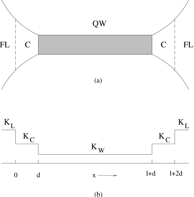
FIG. 1.: Schematic diagram of the model showing the lead regions (marked FL for Fermi liquid), the contact regions (C) of length $d$, and the quantum wire (QW) of length $l$. The interaction parameters in these three regions are denoted by $K_{L}$, $K_{C}$ and $K_{W}$ respectively.

REFERENCES

- [1] S. Tarucha et al., Sol. St. Comm. 94, 413 (1995).
- [2] K. J. Thomas et al., Phys. Rev. Lett. 77, 135 (1996).
- [3] A. Yacoby et al., Phys. Rev. Lett. 77, 4612 (1996).
- [4] C. -T. Liang et al., Phys. Rev. B 61, 9952 (2000).
- [5] A. Kristensen et al., Phys. Rev. B 62, 10950 (2000).
- [6] R. de Picciotto et al., Phys. Rev. Lett. 85, 1730 (2000).
- [7] B. E. Kane et al., App. Phys. Lett. 72, 3506 (1998).
- [8] D. J. Reilly et al., cond-mat/0001174.
- [9] C. L. Kane and M. P. A. Fisher, Phys. Rev. B 46, 15233 (1992).
- [10] I. Safi and H. J. Schulz, Phys. Rev. B 52, 17040 (1995).
- [11] D. L. Maslov and M. Stone, Phys. Rev. B 52, 5539 (1995); V. V. Ponomarenko, ibid. 52, R8666 (1995).
- [12] A. Furusaki and N. Nagaosa, Phys. Rev. B 54, 5239 (1996).
- [13] I. Safi, Ph.D. thesis, Laboratoire de Physique des Solides, Orsay (1996); Ann. Phys. (Paris) 22, 463 (1997); I. Safi and H. J. Schulz, Phys. Rev. B 59, 3040 (1999).
- [14] C. de C. Chamon and E. Fradkin, Phys. Rev. B 56, 2012 (1997).
- [15] M. Bttiker, Phys. Rev. B 41, 7906 (1990).
- [16] K. A. Matveev, Phys. Rev. B 51, 1743 (1995).
- [17] A. Yacoby and Y. Imry, Phys. Rev. B 41, 5341 (1990).
- [18] S. Lal, S. Rao and D. Sen, in preparation.
- [19] I. Safi, Phys. Rev. B 56, R12691 (1997).