Magnons in the ferromagnetic Kondo-lattice model

Abstract

The magnetic properties of the ferromagnetic Kondo-lattice model (FKLM) are investigated. Starting from an analysis of the magnon spectrum in the spin-wave regime, we examine the ferromagnetic stability as a function of the occupation of the conduction band $n$ and the strength $J$ of the coupling between the localised moments and the conduction electrons. From the properties of the spin-wave stiffness $D$ the ferromagnetic phase at zero temperature is derived. Using an approximate formula the critical temperature $T_{c}$ is calculated as a function of $J$ and $n$.

1 Introduction

The intensively investigated Kondo-lattice model (KLM) describes the exchange coupling of the itinerant electrons to a system of permanent, localised magnetic moments. These moments have their origin in the partially filled 5f-, 4f- and 3d-shells of materials such as actinides, rare earth elements, transition metals and their compounds.
The electrons of the conduction band mediate an indirect exchange interaction between the local moments, which order collectively below a critical temperature $T_{c}$. The Hamiltonian of the Kondo-lattice model is defined as follows [1]:

$$H=\sum_{ij\sigma}T_{ij}a_{i\sigma}^{+}a_{j\sigma}-J\sum_{i}{\bf\sigma}_{i}{\bf S}_{i}.$$ (1)

The first term describes the hopping of the conduction electrons between different lattice sites at ${\bf R}_{i}$ and ${\bf R}_{j}$. $T_{ij}$ are the hopping matrix elements, which represent the amplitude of the respective hopping process. The hopping integral is

$$T_{ij}=\frac{1}{N}\sum_{\bf k}\epsilon({\bf k})e^{i{\bf k}({\bf R}_{i}-{\bf R}_{j})},\$$ (2)

where $\epsilon({\bf k})$ is the Bloch dispersion. The operators $a_{i\sigma}^{+}$ and $a_{j\sigma}$ denote the creation and annihilation operators for conduction electrons with spin $\sigma$.
The second term describes the exchange coupling between the system of local moments and the conduction electrons. This term is similar to the Heisenberg Hamiltonian [2] and describes the local character of the interaction. ${\bf\sigma}_{i}$ is the spin operator of the conduction electrons, and ${\bf S}_{i}$ the operator of the localised spins.
A very important fact is the sign of the coupling constant $J$. If $J<0$, the itinerant electrons and the local spins couple antiferromagnetically. One result is the existence of a nonmagnetic phase caused by screening of the local moments [3, 4]. The term “Kondo-lattice model” implies a negative $J$. If $J>0$ the two subsystems couple ferromagnetically. Because the model with positive $J$ differs from the KLM only in the sign of $J$ it is refered to as the “ferromagnetic Kondo-lattice model (FKLM)” or “sf-(sd-) model”.
Interest in the FKLM has been on the increase following the rediscovery of ‘colossal magnetoresistance’ in various manganites, where a large change in resistivity associated with the FM transition occurs.[5]. The first observation of this effect has been made in 1950 [6] Manganites have a perovskite structure R_1-xX_xMnO₃, where R=La, Pr, Nd and X=Sr, Ca, Br, Pb. The manganite La_1-xCa_xMnO₃ is a prototype for the double exchange model [7], which can qualitatively describe ferromagnetism in manganites. However, it cannot reproduce the complex phase diagram of La_1-xCa_xMnO₃, where antiferromagnetic, ferromagnetic and paramagnetic phases as well as phase separation has been observed [5].
A procedure to reproduce this phase diagram using the FKLM has been presented in a paper by Dagotto et al.[8] These authors calculate phase diagrams for one- and two-dimensional systems with different total spins $S$. Both the existence of different magnetic phases and phase separation were demonstrated. A similar phase diagram has been calculated for infinite dimensions [9]. It is generally believed, therefore, that the FKLM is a good starting point for the determination of a phase diagram of manganites even in three dimensions. This is plausible if the $t_{2g}$ electrons of the Mn³⁺ ions in La_1-xCa_xMnO₃ are assumed to be quasilocalised $S=\frac{3}{2}$-spins and the $e_{g}$ electrons are assumed to be itinerant electrons moving through the $S=\frac{3}{2}$ lattice and being ferromagnetically coupled to the localised moments.
Another class of substances which are described by the FKLM are the ferromagnetic metals Gd, Tb, Dy and doped EuX [10]. Gd is an excellent prototype since its total spin of $\frac{7}{2}$ is the largest possible for the rare earth elements. The main focus of this paper are the ferromagnetic metals. In the framework of the FKLM the main difference between these materials and the manganites is the value of of the couplings strength $J$, which is one order of magnitude larger in manganites. The coupling constant in ferromagnetic metals is in the order of 0.1 eV [11].
The main aim of this work is to determine the ferromagnetic phase in three dimensions at $T=0$ K by analysing the stability of the spin-wave spectra. The magnon energies will be calculated by determining the poles of a magnon Green’s function. The same approach has been used by Wang [12], whose numerical results showed two significant properties of spin-wave spectra in the FKLM, namely the vanishing of the acoustic mode in the continuum and the effect of an anomalous softening of the spin-wave dispersion at the edge of the Brillouin zone. The second effect has been experimentally demonstrated in the manganite Pr_0.63Sr_0.37MnO₃ [14]. The author of [12] did not, however, investigate systematically the spin-wave dependence on the coupling strength and the band occupation $n$. The dependence of the spin wave energy on the coupling strength in the FKLM has been calculated by Furukawa for a fixed band occupation. An increase of the magnon energy with increasing coupling strength has been shown [13].
In this work a systematic investigation of the spin wave energy at different band occupations and coupling strengths is presented. From the spin wave stiffness $D$ we can determine the ferromagnetic phase in a $J-n$ diagram in 3D at $T=0$ K. It will be of particular interest to see whether and at what parameter configuration anomalous softening occurs. Finally we calculate the critical temperature dependence on $J$ and $n$ using an approximate formula taken from the Heisenberg model.

2 Theory

In this section we derive the magnon Green’s function for low temperatures in the random phase approximation (RPA). We then discuss briefly the resulting energetic structure of the magnon system.
We use the identities for the electron spin operators ($\hbar$=1)

$$\sigma_{i}^{z}=\frac{1}{2}\sum_{\sigma}z_{\sigma}n_{i\sigma},\sigma_{i}^{+}=a_{i\uparrow}^{+}a_{i\downarrow},\sigma_{i}^{-}=a_{i\downarrow}^{+}a_{i\uparrow},$$ (3)

and for the local moment spin operators

$$S_{i}^{x}=\frac{1}{2}(S_{i}^{+}+S_{i}^{-});\>S_{i}^{y}=\frac{1}{2i}(S_{i}^{+}-S_{i}^{-})$$ (4)

to find a more useful form for the sf-term in Eq.(1)

$$H_{sf}=-\frac{J}{2}\sum_{i,\sigma}(z_{\sigma}S_{i}^{z}n_{i\sigma}+S^{\sigma}_{i}a_{i-\sigma}^{+}a_{i\sigma})$$ (5)

with $\sigma=\uparrow=+,\sigma=\downarrow=-,z_{\uparrow}=1$ and $z_{\downarrow}=-1$. The $S_{i}^{\sigma}$ are the spin flip operators which cause spin deviation in the local moment system.
The first term on the right-hand side of Eq.(5) is an ”Ising-term”, since it describes the interaction of the z-components of localised spins [15]. The second term is non-diagonal in the spin indices and is called the “spin-flip term”.
We want to investigate the properties of our system at very low temperatures. In this limit we can apply the spin-wave approximation using the Holstein-Primakoff transformation [16] . This expression can then be simplified for low temperatures. By applying this approximation to (1) one gets:

$$H=\sum_{ij}T_{ij}a^{+}_{i\sigma}a_{j\sigma}-\frac{J}{2}\left(\sum_{i,\sigma}z_{\sigma}(S-n_{i})n_{i\sigma}+\sum_{i}\sqrt{2S}(b_{i}a_{i\downarrow}^{+}a_{i\uparrow}+b_{i}^{+}a_{i\uparrow}^{+}a_{i\downarrow})\right).$$ (6)

$b_{i}^{+}$,$b_{i}$ are Bose operators. The elementary excitation of the spin system can be derived from the retarded magnon Green’s function $\langle\langle S_{i}^{+};S_{j}^{-}\rangle\rangle_{E}$, which is defined as follows:

$$\langle\langle S_{i}^{+};S_{j}^{-}\rangle\rangle_{E}=-{\rm i}\int_{0}^{\infty}\ {\rm d}t\>exp(-{\rm i}Et)\>\langle[S_{i}^{+}(t),S_{j}^{-}(0)]_{-}\rangle.$$ (7)

$\langle...\rangle$ means thermodynamic averaging, while $[...]_{-}$ denotes the commutator.
In the spin wave approximation, the magnon Green’s function is given by

$$\langle\langle S_{i}^{+};S_{j}^{-}\rangle\rangle_{E}=2S\langle\langle b_{i};b_{j}^{+}\rangle\rangle_{E}.$$ (8)

The equation of motion of $\langle\langle b_{i};b_{j}^{+}\rangle\rangle_{E}$ is

$$E\langle\langle b_{i};b_{j}^{+}\rangle\rangle_{E} = \langle[b_{i},b_{j}^{+}]_{-}\rangle+\langle\langle[b_{i},H]_{-};b_{j}^{+}\rangle\rangle_{E}$$ (9)

$$= \delta_{ij}+\frac{1}{2}J\sum_{\sigma}z_{\sigma}\langle\langle b_{i}n_{i\sigma};b_{j}^{+}\rangle\rangle_{E}-\frac{1}{2}J\sqrt{2S}\langle\langle a_{i\uparrow}^{+}a_{i\downarrow};b_{j}^{+}\rangle\rangle_{E}.$$

On the right-hand side of the equation of motion we have two higher Green’s functions. The spin-flip Green’s function represents a characteristic part of the interaction between electrons and magnons since a magnon is created or annihilated by an electron spin-flip process. These processes are of primary importance in determining the magnetic properties of the FKLM. We therefore decouple the Ising-function only:

$$\langle\langle b_{i}n_{i\sigma};b_{j}^{+}\rangle\rangle_{E}=\langle n_{i\sigma}\rangle\langle\langle b_{i};b_{j}^{+}\rangle\rangle_{E}.$$ (10)

The spin-flip function is treated more carefully. We define a general spin-flip Green’s function $\Gamma_{ik,j}(E)$:

$$\Gamma_{ik,j}(E)=\langle\langle a_{i\uparrow}^{+}a_{k\downarrow};b_{j}^{+}\rangle\rangle_{E}.$$ (11)

If we now apply Eq.(10) to the equation of motion (9) and use the Fourier transform $G_{\bf q}(E)=\langle\langle b_{\bf q};b_{\bf q}^{+}\rangle\rangle_{E}$ of $G_{ij}(E)=\langle\langle b_{i};b_{j}^{+}\rangle\rangle_{E}$ we get the following form of the equation of motion in q-space:

$$EG_{\bf q}(E) = 1+J\langle\sigma^{z}\rangle G_{\bf q}(E)-\frac{J}{2N}\sqrt{2S}\sum_{i,j}e^{-i{\bf q}({\bf R}_{i}-{\bf R}_{j})}\Gamma_{ii,j}(E)$$ (12)

$$\langle\sigma^{z}\rangle = \frac{1}{2N}\sum_{{\bf k},\sigma}z_{\sigma}\langle n_{{\bf k}\sigma}\rangle.$$ (13)

We now derive the equation of motion for $\Gamma_{ik,j}(E)$:

$$E\Gamma_{ik,j}(E) = \langle[a_{i\uparrow}a_{k\downarrow},b_{j}^{+}]_{-}\rangle+\langle\langle[a_{i\uparrow}a_{k\downarrow},H]_{-};b_{j}^{+}\rangle\rangle_{E}$$

$$= \sum_{n}(T_{kn}\Gamma_{in,j}(E)-T_{ni}\Gamma_{nk,j}(E))+JS\Gamma_{ik,j}(E)$$

$$- \frac{J}{2}\left(\langle\langle n_{k}a_{i\uparrow}^{+}a_{k\downarrow};b_{j}^{+}\rangle\rangle_{E}+\langle\langle n_{i}a_{i\uparrow}^{+}a_{k\downarrow};b_{j}^{+}\rangle\rangle_{E}\right)$$

$$- \frac{J}{2}\sqrt{2S}\left(\langle\langle b_{k}a_{i\uparrow}^{+}a_{k\uparrow};b_{j}^{+}\rangle\rangle_{E}-\langle\langle b_{i}a_{i\downarrow}^{+}a_{k\downarrow};b_{j}^{+}\rangle\rangle_{E}\right).$$

On the right-hand side of Eq.(2) we have a set of higher Green’s function which describe more complex interaction processes between itinerant electrons and magnons. These higher Green’s functions are RPA decoupled, preserving spin and particle conservation, as follows:

$$\langle\langle n_{k}a_{i\uparrow}^{+}a_{k\downarrow};b_{j}^{+}\rangle\rangle_{E} \approx \langle n_{k}\rangle\Gamma_{ik,j}(E)$$

$$\langle\langle b_{k}a_{i\uparrow}^{+}a_{k\uparrow};b_{j}^{+}\rangle\rangle_{E} \approx \langle a_{i\uparrow}^{+}a_{k\uparrow}\rangle G_{kj}(E).$$ (15)

Applying the Fourier transform of the spin-flip Green’s function to 2 we and using Eq.(2) we obtain the following approximate expression for the equation of motion:

$$\Gamma_{{\bf k,q^{\prime}}}(E)=-\frac{J\sqrt{2S}}{2\sqrt{N}}\frac{(\langle n_{{\bf k}\uparrow}\rangle-\langle n_{{\bf k+q^{\prime}}\downarrow}\rangle)\>G_{\bf q^{\prime}}(E)}{E-\epsilon({\bf k+q^{\prime}})+\epsilon({\bf k})-J(S-\frac{1}{N}\sum_{\bf p}\langle n_{\bf p}\rangle)}.$$ (16)

At this stage we can obtain an analytical expression of the magnon Green’s function by solving Eq.(12):

$$G_{\bf q}(E)=\frac{1}{E-J\langle\sigma^{z}\rangle-J^{2}S\chi({\bf q},E)}$$ (17)

where

$$\chi({\bf q},E)=\frac{1}{2N}\sum_{\bf k}\frac{\langle n_{{\bf k}\uparrow}\rangle-\langle n_{{\bf k+q}\downarrow}\rangle}{E-\epsilon({\bf k+q})+\epsilon({\bf k})-J(S-\frac{1}{N}\sum_{\bf p}\langle n_{\bf p}\rangle)}$$ (18)

and $\langle n_{\bf p}\rangle$ is the occupation number of the magnons. At very low temperatures the number of magnons in the system is very small since the system is almost saturated ferromagnetically. We therefore set $\langle n_{\bf p}\rangle=0$ for numerical simplicity.
In [12] the magnon Green’s function $\langle\langle S^{+}(-{\bf q});S^{-}({\bf q})\rangle\rangle$ is derived by solving the equation of motion for finite temperatures in RPA. If we set $\langle S^{z}\rangle=S$ in this more general expression, our result with $\langle n_{\bf p}\rangle=0$ and ${\bf q}=-{\bf q}$ is obtained.
In the RPA theory, the magnon energy is renormalised by the term $\chi({\bf q},E)$, which is due to electron-magnon interaction. This term is given explicitly by the band structure, the occupation of the electron system and the coupling strength.
In this work we wish to investigate the energetic structure of the magnons. The magnitude of the dispersion is influenced by the real part of the magnon self energy, while the magnon lifetime is described by its imaginary part. The self energy $M_{\bf q}(E)$ can be defined by the formal solution of the retarded magnon Green’s function

$$G_{\bf q}^{ret}(E)=\frac{1}{E-M_{\bf q}(E)+i0^{+}}.$$ (19)

The magnon self energy in RPA can now be derived from Eq.(17):

$$M_{\bf q}(E)=J\langle\sigma^{z}\rangle+J^{2}S(Re\chi({\bf q},E)+iIm\chi({\bf q},E)).$$ (20)

By applying the Dirac identity we can calculate the real and imaginary part of $\chi({\bf q},E)$:

$$Re\chi({\bf q},E)=\frac{1}{2N}{\cal P}\sum_{\bf k}\frac{(\langle n_{{\bf k}\uparrow}\rangle-\langle n_{{\bf k+q}\downarrow}\rangle)}{E-\epsilon({\bf k+q})+\epsilon({\bf k})-JS},$$ (21)

$$Im\chi({\bf q},E)=\frac{-\pi}{2N}\sum_{\bf k}(\langle n_{{\bf k}\uparrow}\rangle-\langle n_{{\bf k+q}\downarrow}\rangle)\delta(E-\epsilon({\bf k+q})+\epsilon({\bf k})-JS)$$ (22)

where ${\cal P}$ denotes the principal value. This gives rise to two collective excitation modes and a one particle continuum as discussed in [17].
Outside this continuum the principal value at the right-hand side of eq. (21) is equal to the function itself, the imaginary part vanishes and the magnon lifetime becomes infinite. The poles of the Green’s function, i.e. the collective excitation energies, are then defined by the implicit equation

$$E-J\langle\sigma^{z}\rangle-J^{2}SRe\chi({\bf q},E)\stackrel{{\scriptstyle!}}{{=}}0.$$ (23)

The stability of the local moment ferromagnet at low temperature is determined by the collective excitations from the ferromagnetic ground state. The excitations into the acoustic mode are certainly dominant. We therefore limit ourselves to an analysis of the dependence of the acoustic mode on $J$ and $n$.
In order to solve Eq.(23) an expression for the $\langle n_{\bf{k}\sigma}\rangle$ is required. It is very common to treat the electronic system in a mean-field approximation (see e. g. [17]). This leads to a situation in which the electron-magnon interaction is included in the investigation of the magnon system, but not of the electronic system. In this work we wish to investigate how the ferromagnetic properties of our model system are determined by the RPA theory. We therefore limit ourselves to a mean-field treatment of the electronic part. In this approximation the expectation values of the ${\bf k}$-dependent occupation numbers in Eq. (21) is

$$\langle n_{{\bf k}\sigma}\rangle=\frac{1}{e^{\beta(\epsilon({\bf k})-\mu-\frac{1}{2}Jz_{\sigma}S)}+1}.$$ (24)

In this work we assume the system to be a simple cubic lattice with nearest-neighbor interaction only. The electronic dispersion of such a system is given by

$$\epsilon({\bf k})=-2t\sum_{i=1}^{d}cos(k_{i})+t_{0},\>k_{i}\>\epsilon[-\pi;\pi],\>t>0.$$ (25)

The midpoint of the band $t_{0}$ is chosen to be zero. The relation between the band width $W$ and the hopping term $t$ is $W=12t$.

3 Results and Discussion

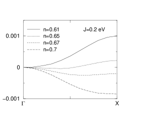
Figure 2: Spin-wave dispersion $E({\bf q})$ in [100] direction for a system with $S=3.5$, band width $W=1.0$ eV at $T=0$ K. The dispersions for two different coupling constants $J=0.2$ eV and $J=0.25$ eV at different band occupations $n$ are shown.

In this section we discuss the properties of the spin-wave dispersion Eq.(23) with increasing band occupation $n$ at different values of the coupling $J$. The coupling of the conduction electrons to the local moments leads to an indirect interaction between the spins.
In Fig. 1 spin wave spectra in the [100] direction are sketched for $J=0.2eV$ and $J=0.25eV$ at different band occupations $n$. By filling the conduction band with electrons the magnon energy increases up to a maximum at a given band occupation $n$. This maximum value increases with increasing $J$. After reaching the maximum value close to the quarter-filled band, the magnon energy decreases monotonically with further increasing band occupation.
The excitation energy of a spin-wave mode is the energy needed to cause a deviation of the spin system of unity from the ferromagnetically saturated state. Hence the larger the spin-wave energy the larger the ferromagnetic stability. This is of course a qualitative statement which must be substantiated by quantitative calculation of, for example, the critical temperature $T_{c}$.
In Fig. 2 we have sketched the behaviour of the magnon energies by further increasing the band occupation. The spin-wave spectra become negative.
The existence of negative excitation energies is of course unphysical since the magnons are excitations from the ground state. There is thus no stable ferromagnetic ground state beyond a critical band occupation $n_{c}$. The determination of $n_{c}$ requires the definition of a stability condition. The system becomes ferromagnetically unstable if the magnon energy becomes negative.
A widely used parameter for the ferromagnetic stability is the spin-wave stiffness $D$. In [12] it has been shown that the expression for the magnon energy can be rewritten as $E({\bf q})=D{\bf q}^{2}$ for small $q$. When $D$ becomes zero the system becomes ferromagnetically unstable. In the intermediate coupling regime $0.2eV<J<0.7eV$, this is indeed a unique criterion since the spin-wave energy becomes zero at small $q$.
However, an interesting effect can be observed at very small $J$. In Fig. 3 the magnon spectra for a system with $J=0.1$ eV are sketched. At $n=0.24$ the spin-wave dispersion starts to decrease significantly for large $q$ while the spin-wave stiffness remains almost the same. This effect is known as ’anomalous softening’. A second minimum appears in the dispersion curve at the righthand edge of the Brillouin zone. At $n=0.255$ the spin-wave energy at the $X$-point becomes zero. Hence at small $J$ a ferromagnetic instability exists at large $q$.
This effect has been observed experimentally in the manganite Pr_0.63Sr_0.37Mn0₃ [14]. But in manganite systems a strong coupling between the conduction electrons and the localised moments exists. It is thus not very clear, whether or not the anomalous softening found in our calculation is comparable to the experimental results. A more complex theory which assumes some d-character of the conduction electrons has already been presented in order to explain the measured anomalous softening [18]. A reasonably good agreement between theory and experimental data has been found. Despite this unsolved problem anomalous softening is certainly a model property of the FKLM as well. A very significant consequence of anomalous softening is the fact that the spin-wave stiffness $D$ is almost constant while the magnon energy at large $q$ is lowered. The decrease in magnon energy is equivalent to a decrease in ferromagnetic stability and hence of the critical temperature $T_{c}$. In our theory these facts would lead to an increase of the relation $\frac{D}{T_{c}}$. This effect has also been observed experimentally in manganite systems [19]. In this paper a ferromagnetic ground state is assumed. It is thus only possible to report a unique ferromagnetic instability at $J=0.1$ eV. The cause of the anomalous softening at low $J$ and hence the nature of the new phase is currently the subject of further research.
We have defined above the critical band occupation $n_{c}$ where the spin-wave stiffness becomes zero and the system ferromagnetically unstable. By calculating $n_{c}$ at different coupling $J$ we can sketch the ferromagnetic phase in a $J-n$ diagram, shown in Fig. 4.
The ferromagnetic phase occupies a large part of the phase diagram. The critical band occupation increases by increasing the coupling strength $J$. There is no ferromagnetism around half filling $(n=1)$. One gets a qualitative explanation of this result by looking at the energy of different spin states of the conduction electrons at half filling. All lattice points are occupied with one electron. If all electrons are in the spin-up state, no virtual hopping between the lattice points is possible. Virtual hopping reduces the energy of the system. Thus the stable spin configuration corresponds to the state with the maximal hopping amplitude, i.e. where all nearest neighbour electrons have opposite spin. Since we assume a ferromagnetic coupling between the two electron subsystems, such a spin configuration corresponds to an antiferromagnetic order of the local moments.
At $J=0.1$ eV we have sketched two points. The black point represents the band occupation where the magnon energy vanishes at the right-hand edge of the Brillouin zone. The second point is sketched at $n_{c}$. Hence the procedure described to determine the phase border is no longer unique.
The structure of the ferromagnetic phase of our system is very similar to those calculated in [8] and [9]. These calculations were performed using a variety of different methods, such as quantum Monte Carlo calculations, for systems with different dimensions d and total spins $S$. It is therefore quite problematic to compare these phase diagrams directly. However the similarity between these results is remarkable. The qualitative behaviour of the ferromagnetic phase seems to be a general property of the FKLM.
Finally we have calculated the critical temperature using an approximate formula which can be derived from the spin-wave approximation of the Heisenberg model (see e. g. [7]):

$$k_{B}T_{c}=\left(\frac{1}{NS}\sum_{\bf q}\frac{1}{E({\bf q})}\right)^{-1},$$ (26)

where $E({\bf q})$ is the spin-wave dispersion of a local moment system with direct exchange interaction.
This formula extrapolates the critical temperature from the magnon energy of the system in the spin-wave regime. A quantitatively better calculation of the critical temperature would require a self-consistent calculation.
At this stage we can only give a qualitative description of the dependence of the critical temperature on the band occupation $n$ and the coupling strength $J$. In our system the exchange interaction is mediated by the conduction electrons. The FKLM-Hamiltonian can be mapped onto an effective Heisenberg-Hamiltonian [11]. Information about the kind of interaction is then buried in the effective exchange integrals $J({\bf q})$, which are functionals of the electronic self energy. This description leads to the modified RKKY-interaction [11]. Following the same idea we can describe the excitation of the local spins in the spin-wave approximation as a system of noninteracting magnons:

$$H=E_{0}+\sum_{\bf q}\Omega_{eff}^{RPA}({\bf q})b_{\bf q}^{+}b_{\bf q}.$$ (27)

E(q)=$\Omega_{eff}^{RPA}({\bf q})$ is the spin-wave dispersion (23). The renormalised spin-wave energies are equivalent to the effective exchange integrals in the modified RKKY-interaction [11]. In our theory we can therefore rewrite the approximate formula (26) for the critical temperature.

$$k_{B}T_{c}=\left({\frac{1}{NS}}\sum_{\bf q}\frac{1}{\Omega_{eff}^{RPA}({\bf q})}\right)^{-1}$$ (28)

This equation is used to calculate the dependence of the critical temperature by evaluating the magnon energies in the whole Brillouin zone for given $n$ and $J$.
Plots of $T_{c}$ versus $n$ for different $J$ are sketched in Fig. 5. From Eq. (28) it is evident that the functional dependence of $T_{c}$ is equivalent to the $n$-dependence of the magnon energy. The critical temperature increases by increasing the band occupation up to a maximum. After passing this maximal value the critical temperature decreases monotonically before it vanishes at the critical band occupation $n_{c}$ (black points). Since the error of the numerical evaluation of $T_{c}$ becomes very large near the critical band occupation, the value of $n_{c}$ was taken from the phase diagram in Fig. 4. The good agreement between the $T_{c}$ versus $n$ graphs and the respective $n_{c}$ values supports the stability condition using the spin-wave stiffness $D$ defined above. Good qualitatitive agreement with the $T_{c}$ dependence on $n$ reported in [11] has been found. This agreement is perhaps unexpected, since a more realistic description of the electronic system is used in [11]. This could be due to the fact that the exchange integrals used in [11] are to first order very similar to the expression of the real part of $\chi({\bf q},E)$ in Eq.(21) which renormalises the expression of the magnon energy Eq. (23) with respect to electron-magnon interaction. The qualitative behaviour of the critical temperature is mainly determined by these interaction processes. It is thus reasonable that the inclusion of those processes in the perturbative analysis of the magnon system leads to a good description of the qualitative behaviour of $T_{c}$.
An exception is the $T_{c}(n)$ dependence at $J=0.1$eV. The calculation stopped at $n=0.21$. Above this band occupation we have to sum over two singularites in Eq.(28) due to the effect of anomalous softening. A numerical calculation is now rather complicated and was not done at this stage. However we sketched the critical band occupation $n_{c}=0.38$, where the spin-wave dispersion at small values of $q$ vanishes. If we assume the same qualitative dependence of $T_{c}$ as found for the larger $J$ this $n_{c}$ is too large. Hence the stability condition using $D$ does not work at this $J$.
A similar qualitative dependence of the critical temperature, on the band occupation, including a maximum at quarter filling, has also been found for the strong coupling limit ($J\rightarrow\infty)$ of the FKLM assuming classical spin ($S=1$) and using Monte-Carlo methods [20].
Another interesting result concerns the critical temperature as a function of the coupling strength $J$ in Fig. 6. It is sketched for three different band occupations $n$. The $T_{c}$ versus $J$ dependences for $n=0.1$ and $n=0.06$ are quite similar. The critical temperature increases with increasing coupling strength $J$. This result is intuitively correct. For $n=0.4$ we found a critical coupling strength $J_{c}$. Below $J_{c}$, $T_{c}$ is zero and the system is not ferromagnetically ordered. The existence of a $J_{c}$ has also been shown in [11] for higher band occupations. A different qualitative behaviour compared to [11] has been found at large $J$. While in that work $J$ remains constant above a certain value, we did not find saturation. This difference could be caused by the different electronic self energies used. We have not calculated the critical temperature for $J<0.1$eV. For this region we expect the normal RKKY-behaviour $T_{c}\sim J^{2}$, as shown in [11].

4 Summary and Conclusions

We have investigated the ferromagnetic properties of the FKLM through an analysis of the spin-wave spectrum at very low temperature. The spin-wave approximation was applied to the model Hamiltonian and the magnon Green’s function was derived within the RPA approximation. The numerical analysis of the magnon energy spectrum was limited to the acoustic branch of the collective excitations.
The results of $n$- and $J$-dependent calculations of the magnon spectra have been presented. The magnon energy for fixed coupling strength $J$ increases with increasing occupation of the conduction band up to a maximum value close to quarter filling. After reaching the maximum value the energy decreases as n increases and eventually vanishes. A stability condition for the ferromagnetic state was defined by using the spin-wave stiffness $D$. If the magnon energy at small $q$ vanishes at the critical band occupation $n_{c}$, i.e. $D$ becomes zero, the system becomes ferromagnetically unstable. The ferromagnetic phase in three dimensions has been determined by calculating $n_{c}$ for different $J$. There is a good agreement to the ferromagnetic phase obtained for FKLM-model systems with different total spin $S$ and dimension $d$ in [8] and [9]. The critical band occupation $n_{c}$ increases by increasing the coupling strength. There is no ferromagnetism around $n=1$. The good agreement between the different calculations may lead to the conclusion that the structure of the ferromagnetic phase is a general property of the FKLM.
In addition anomalous softening is found at $J=0.1eV$. The method to determine $n_{c}$ is thus no longer unique. It is not yet possible to link this result to the anomalous softening observed experimentally. This problem as well as the physical reason of this phenomenon is an interesting subject of future research.
Finally the critical temperature dependence on $J$ and $n$ was presented. A qualitative agreement to the results shown in [11] was found. A more careful treatment of the electronic system and a selfconsistent calculation of the critical temperature is currently the subject of further research.

Figure 1: Spin-wave dispersion $E({\bf q})$ in [100] direction for a system with $S=3.5$, band width $W=1.0$ eV at $T=0$ K. The dispersions for two different coupling constants $J=0.2$ eV and $J=0.25$ eV at different band occupations $n$ are shown. On the left-hand side of the figure the magnon energy increases with increasing n, whilst at the right-hand side it decreases.

Figure 3: Spin-wave dispersion $E({\bf q})$ in [100] direction for a system with $S=3.5$, band width $W=1.0$ eV at $T=0$ K. The dispersion for different $n$ at $J=0.1$ eV are shown.

Figure 4: Ferromagnetic phase at $T=0$ K, $S=3.5$, and $W=1.0$ eV

Figure 5: Critical Temperature $T_{c}$ as a function of $n$ at different coupling constants $J$.

Figure 6: Critical Temperature $T_{c}$ as a function of $J$ at different band occupations $n=0.06,~{}0.1,~{}0.4$.

References

- [1] C. Zener, Phys. Rev 81, 440 (1951).
- [2] W. Heisenberg, Z. Phys. 49, 619 (1928).
- [3] C. Lacroix and M. Cyrot, Phys. Rev. B. 20, 1969 (1928).
- [4] C. Lacroix, Solid State Comm. 54, 991 (1985).
- [5] Review by A.P. Ramirez, J. Phys: Condens. Matter 9, 8171 (1997) and references within.
- [6] G.H. Jonker, J.H. Van Santen, Physica 16, 337 and 559 (1950)
- [7] W. Nolting, Quantentheorie des Magnetismus, Teil 2. Modelle, (Stuttgart, Teubner, 1986).
- [8] E. Dagotto et.al., Phys. Rev. B. 58, 6416 (1998).
- [9] T. Momoi, K. Nagai and K. Kubo, arxiv: cond-mat/9911091 (1999).
- [10] M. Donath, P.A. Dowben and W. Nolting (ed.), Correlations in Local-Moment Systems: Rare-Earth Elements and Compounds, World Scientific (1998).
- [11] W. Nolting, S. Rex and S. Mathi Jaya, J. Phys: Condens. Matter 9, 1301 (1996).
- [12] X. Wang, Phys. Rev. B. 57, 7427 (1998).
- [13] N. Furukawa, J. Phys. Soc. 65, 1174 (1996)
- [14] H.Y. Hwang et.al., Phys. Rev. Lett. 80, 1316 (1998).
- [15] E. Ising, Z. Phys. 31, 253 (1925).
- [16] T. Holstein and W. Primakoff, Phys. Rev. 58, 1048 (1940).
- [17] A. Babcenko and M.G. Cottam, J. Phys. C 14, 5347 (1981).
- [18] G. Khalliulin and R. Killian, arxiv: cond-mat/9910106 (1999).
- [19] J.A. Fernandez-Baca et.al., Phys. Rev. Lett. 80, 4012 (1998).
- [20] S. Yunoki et.al., Phys. Rev. Lett. 80, 845 (1998).