[

Force Dependence of the Michaelis Constant in a Two–State Ratchet Model for Molecular Motors

Abstract

We present a quantitative analysis of recent data on the kinetics of ATP hydrolysis, which has presented a puzzle regarding the load dependence of the Michaelis constant. Within the framework of coarse grained two–state ratchet models, our analysis not only explains the puzzling data, but provides a modified Michaelis law, which could be useful as a guide for future experiments.

]

Molecular motors or protein motors are the terms used to describe a highly specialized class of enzymes which transduce the energy excess in the chemical hydrolysis reaction of ATP (adenosinetriphosphate) into mechanical work. They are involved in several important cellular processes, ranging from the transport of material and vesicles, to cell mobility and cell division. Linear protein motors move along complex periodic and polar structures called filaments, obtained by the polymerization of a single monomer (actin) or dimer (microtubules) [1, 2].

Several models have been proposed so far to explain the energy transduction process. In the earliest ones, known as cross–bridge models [3, 4], the motor can exist in different states (up to 5 or 6 [5]), within each of which the system reaches local thermodynamic equilibrium on time scales small compared to the exchange rates between the states. This hypothesis relies on the fact that the characteristic times of the motors (measured through transient response [6]) are of the order of milliseconds, while thermal equilibrium on a length scale of about 10 nm occurs in 10-100 ns [7, 8]. The latest models [9, 10, 11, 12, 13, 14, 15] share some common features: i) need for asymmetry (polarity) in order to establish a certain preferred direction of motion; ii) chemical energy consumption as a source of mechanical work; iii) local thermodynamic equilibrium for each state. A particular promising approach is that due to Vale and Oosawa [16], using the ratchet concept introduced by Feynman [17]. Since then, ratchet models have been intensively studied [9, 10, 18]. Non–equilibrium thermodynamics as well as stochastic methods contribute to the theoretical background of this new field of research.

The role of force in the reaction kinetics is still an open question, [19, 20, 21]. In particular, recent experiments performed on kinesin (a processive motor), [21], seem to indicate that the kinetics of ATP hydrolysis can be described by the Michaelis–Menten mechanism. This simple mechanism, introduced in 1913 to describe the process of enzymatic catalysis [22], assumes that the catalytic reaction of a substrate $S$ is divided into two processes. The enzyme $E$ and the substrate first combine rapidly and reversibly to give an enzyme–substrate complex $ES$ with no chemical change on the substrate. The chemical reaction occurs in a second step with a first–order rate constant $k_{cat}$, or turnover number. It is then simple to show that the reaction velocity $r$ (or rate of $S$ consumption) is given by the Michaelis law:

$$r=\frac{r_{max}\ [S]}{K_{M}+[S]},$$ (1)

where $r_{max}$ is a saturation value and $K_{M}$ is called the Michaelis constant. For the ATP hydrolysis reaction, $[S]$ is simply replaced by $[ATP]$. Furthermore it is reasonable that the velocity of a molecular motor should depend strictly on the rate of ATP consumption [7], so that the velocity curve is given by a Michaelis law in terms of ATP concentration. This hypothesis has been tested in the experiment [21] at least for high ATP concentrations. According to these experimental findings the Michaelis law can be written as:

$$v=\frac{\epsilon\ p\ k_{cat}\ [ATP]}{K_{M}+[ATP]},$$ (2)

where $p$ is the periodicity of the filament, $k_{cat}$ is the turnover number, and $\epsilon$, the coupling ratio, gives an estimate of the average performance of one hydrolysis event, i.e. it is higher when the energy transduction process is more efficient. It is rather intuitive that the coupling ratio should depend on the applied force, and should decrease when the opposing force is increased, as the applied load strongly limits the maximum attained velocity on which the coupling ratio is linearly dependent. The rather surprising experimental finding [21] is that the Michaelis constant $K_{M}$ is no longer a constant, but increases with increasing applied load. This result is not intuitive and rather striking, since the Michaelis constant is just an equilibrium constant for the reaction leading to the formation of the enzyme-substrate complex. Indeed reaction rates are assumed to be independent of the external force as long as they do not contribute to a net motion of the motor. Thus this experimental finding makes the picture more complicated than expected. It was suggested in [21] that a possible explanation might be to insert the external force in the transition rates as done by Fisher and Kolomeisky [20], but this cannot be done unambiguously, as stated by the authors themselves.

Coarse–grained two-state ratchet models [18] can give further insight into this problem. In these models, the state of the motor is indicated by the index $i$, whereas $x$ is the position of the protein center of mass along the track. The chemical reactions force the motor protein to switch from one state $i$ at position $x$ to another state $j$ in the same position $x$, with a rate given by $\omega_{ij}(x)$. The motor moves under the influence of a potential $W_{i}(x)$ chosen so as to reproduce the interaction between the filament and the motor head and with the same characteristics as the filament: polarity and periodicity. For this reason the potential is chosen to be asymmetric and periodic with period $p$ for each state $i$ (“ratchet” potential, see Fig. 1).

In a Fokker–Planck (FP) description, $P_{i}(x,t)$ is the probability density for the particle to be in state $i$ at position $x$ at time $t$, while the probability current $J_{i}(x,t)$ is defined as:

$$J_{i}(x,t)=-\frac{D_{i}}{kT}\left[P_{i}(x)\partial_{x}W_{i}-P_{i}(x)F_{ext}+kT\partial_{x}P_{i}(x)\right]$$ (3)

where $D_{i}$ is a diffusion coefficient which is taken to be equal in both states, $T$ is the temperature, $k$ is the Boltzmann constant and $F_{ext}$ is the external force. Since we are dealing with a simple two-state model, the chemical reaction cycle is compressed in a two step process:

$$\begin{array}[]{ccc}&{\scriptstyle\alpha_{1}(x)}&\\ M+ATP&{\textstyle\rightleftharpoons}&M\cdot ADP\cdot P\\ &{\scriptstyle\alpha_{2}(x)}&\end{array}$$ (4)

$$\begin{array}[]{ccc}&{\scriptstyle\beta_{1}(x)}&\\ M+ADP+P&{\textstyle\rightleftharpoons}&M\cdot ADP\cdot P\\ &{\scriptstyle\beta_{2}(x)}&\end{array}$$ (5)

where $M$ refers to the motor. This strongly resembles the Michaelis–Menten mechanism. The only difference, in this case, is that transition rates depend on the coordinate of the protein center of mass. We emphasize that all of the following discussion does not involve any hypothesis regarding enzymatic catalysis.

The state $M\cdot ADP\cdot P$ corresponds to one in which the motor head is detached from the fiber after binding and dissociating ATP. In this state the motor may move more or less freely upon the filament. This state will be called the “free” state, or state $2$. All the other terms in the equations refer to a state in which the motor is attached to the filament and therefore its motion is strongly dependent on the motor–filament interaction. This is the so called “bound” state or state $1$. In this case we are dealing essentially with a single–headed motor, although the mechanism for a two–head motor protein is similar. We assume detailed balance to hold for each chemical reaction:

$$\frac{\alpha_{1}(x)}{\alpha_{2}(x)}=\exp\left(\frac{W_{1}(x)-W_{2}(x)+\Delta\mu}{kT}\right)$$ (6)

$$\frac{\beta_{1}(x)}{\beta_{2}(x)}=\exp\left(\frac{W_{1}(x)-W_{2}(x)}{kT}\right)$$ (7)

where $\alpha_{1},\alpha_{2}\ (\beta_{1},\beta_{2})$ are the transition rates for the first (second) chemical reaction and $\Delta\mu=\mu_{ATP}-\mu_{ADP}-\mu_{P}$ is the difference in chemical potential or the chemical driving force.

The FP equation describing the process may now be written as:

$$\partial_{t}P_{i}+\partial_{x}J_{i}=\sum_{j\neq i}\left(\omega_{ji}P_{j}-\omega_{ij}P_{i}\right)$$ (8)

where $i=1,2$ for the two-state model and $\omega_{ij}(x)=\alpha_{i}(x)+\beta_{i}(x)$.

The main advantage of this approach is the straightforward manner in which external forces, if any, may be directly inserted in eq. (3) without any need for further assumptions (for a discussion of this point see [20]). If the external force is independent of time, it is possible to look for a stationary solution. The velocity of the motor, $v$, defined as:

$$v=\int_{0}^{p}\left(J_{1}(x)+J_{2}(x)\right)dx,$$ (9)

and the rate of ATP consumption:

$$r=\int_{0}^{p}\left(\alpha_{1}(x)P_{1}(x)-\alpha_{2}(x)P_{2}(x)\right)dx,$$ (10)

where $p$ is the periodicity of the filament, are identically zero when both $\Delta\mu$ and $F_{ext}$ are zero [18]. A necessary condition for motion to occur [18] is that $\Delta\mu\neq 0$, i.e. detailed balance is violated, and that the potential is asymmetric. This implies that the chemical reaction of ATP hydrolysis is able to break detailed balance for the total transition rates.

Using eq. (6) and (7) only two of the four functions $\alpha_{1}(x),\alpha_{2}(x),\beta_{1}(x),$ and $\beta_{2}(x)$, can be chosen arbitrarily once $W_{1}$ and $W_{2}$ are fixed. Since the release of products is just a thermal process and does not involve chemical reactions (see eq. (5)), we assume it to be position independent as in [8], so that $\beta_{2}(x)=\omega=const$.

Transitions due to chemical reactions are usually chosen to be localized, i.e. they may take place only in correspondence to a certain motor position along the filament period and therefore they are not distributed over the whole period. This corresponds to the “active site” concept in biology and in [18] the former hypothesis is shown to agree with experimental data. To take this effect into account we also define:

$$\alpha_{2}(x)=\left\{\begin{array}[]{ll}\omega&\mbox{for }p-\delta<x<p,\\ 0&\mbox{otherwise.}\end{array}\right.$$ (11)

with $\delta/p=0.05$. We use two kinds of models, differing only in the choice of the potential in state $2$ [18, 8]. $W_{1}$ is the standard ratchet potential shown in fig. 1. In model $(a)$, we suppose state $2$ to be strictly diffusive so that the potential $W_{2}(x)$ is flat (Fig.1). This corresponds to the picture of state $2$ as a totally free state. In model (b), we suppose the filament to affect the protein movement, so that the potential in state $2$ is essentially the same as $W_{1}(x)$, except for a uniform offset and a 5 times smaller amplitude of variation. We expect the motion in model (b) to be more constrained than in model (a).

We analyzed the two models $(a)$ and $(b)$ seeking the non–equilibrium stationary solutions $P_{i}^{s}(x)$ to the FP equations when applying different mechanical and chemical driving forces. This has been accomplished by numerically integrating the stationary FP eq. (3) starting from the equilibrium Boltzmann solutions and changing smoothly and alternatively the parameters $\Delta\mu$ and $F_{ext}$. For each stationary solution we calculated the velocity and the rate of ATP consumption. Fig. 2 shows the results for the rate of ATP consumption.

These results are plotted in terms of the ratio:

$$q=\frac{[ATP]}{[ADP][P]}=\exp\left(\frac{\Delta\mu}{kT}\right)$$ (12)

from mass–action law, using concentrations normalized with respect to their equilibrium value. Usually the Michaelis law is written in terms of ATP concentration, while in our results we derive it in terms of the parameter $q$ defined above. We observe that experiments are usually performed in conditions of high ATP concentrations, so that the ratio $q$ can be safely thought to be constant during the time taken by the experiment. Since the only way of varying $q$ is by adding ATP molecules to the solution, $q$ or $[ATP]$ may be interchanged in the Michaelis law. The rate of ATP consumption can be fitted by a Michaelis law in the form:

$$r=\frac{q\cdot r_{MAX}}{K_{M}+q}.$$ (13)

The value $r_{MAX}$ is weakly dependent on the applied force. Our calculations show that the Michaelis–Menten law is followed with a rather impressive precision for $q\gtrsim 10^{3}$, where $1/r$ is linear in $1/q$ with regression coefficients practically equal to $1$. The fact that the Michaelis law is so strictly followed also when different forces are applied is a good indication that the simplified two–state model is still in accordance with well established results for enzymatic catalysis.

Figure 3 shows the velocity as a function of $q$; at first sight these curves seem Michaelis-like, so that the correct equation for velocity should be eq. (13) with $r_{MAX}$ replaced by $v_{MAX}$. In this case $v_{MAX}$ strongly depends on the applied force, and it decreases when the applied force becomes more and more negative. Our results show that the velocity is linear with $r$, so that $v=\alpha r-\beta$ with a regression coefficient always $\gtrsim 0.9996$ and thus the relation for velocity, using eq. (13), reads:

$$v=\frac{\alpha r_{MAX}\cdot q}{K_{M}+q}-\beta.$$ (14)

A pleasing feature is that, using this equation, there is only one Michaelis constant for both $v$ and $r$. Another very interesting point is that the obtained positive values of $\beta$ indicate that ATP consumption is even possible under stall conditions ($v=0$) [23]. This “idling” rate of ATP consumption should be tested by motility assays.

The Michaelis law is commonly thought to hold for very high ATP concentrations. The experimental results [21] were obtained in this regime and fitted using eq. (14) forcing $\beta=0$. Table I shows the results obtained by fitting our numerical data using eq. (14) with $\beta$ as a free parameter; these results are compared with the ones obtained in a fit with a standard Michaelis law, i.e. forcing $\beta=0$. In the former case the fit is extremely good; indeed the sum of square residuals can be hundreds times less than in the latter case. While the maximum attained velocity is essentially independent of the fitting, the results for the Michaelis constant are quite different. The range of variability of $K_{M}$ with $F_{ext}$ is much wider using a standard Michaelis law; this is also confirmed by simple analytical arguments. Furthermore, in the case of model $(b)$ for high loads it is even impossible to fit the data without introducing $\beta$ in eq. (14). Still, eq. (2) does not allow for any inversion in the sign of velocity, nor for a stall condition, at variance with eq. (14).

In conclusion, our calculations on the two-state ratchet model clearly show that the rate of ATP consumption strictly follows a Michaelis law in the form (13); that the correct law for velocity is given by eq. (14), instead of eq. (2); that the observed fourfold increase of the Michaelis constant with applied load may be due to the use of eq. (2); that the model still accounts for an increase of the Michaelis constant smaller than $20\%$ when forces vary by a factor $5$ (in the range of pN), to be compared with the corresponding variation of about $250\%$ if a standard Michaelis law, eq. (2), is used.

We thank F. Cecconi and P. Ván for useful discussions. GL also acknowledges INFM funding.

$F_{ext}$	$K_{M}\ \$	$K^{\prime}_{M}$	$v_{MAX}$	$v^{\prime}_{MAX}$
$0.0$	$238030$	$243710$	$3.9053$	$3.9067$
$-1.0$	$249970$	$254680$	$3.079$	$3.0573$
$-2.0$	$263440$	$268840$	$2.316$	$2.2726$
$-3.0$	$272320$	$292800$	$1.584$	$1.5541$
$-4.0$	$282930$	$360000$	$0.9453$	$0.899$
$-5.0$	$296040$	$\sim 900000$	$0.3886$	$0.295$

TABLE I.: Michaelis constants, $K_{M}$, and maximum velocities, $v_{max}=\alpha\ r_{max}$ calculated from model $(a)$ using eq. (14) (second and fourth columns) with $\beta$ as a free parameter and the same equation with $\beta=0$ (third and fifth columns) corresponding to the standard Michaelis law. In the latter case, the constants $K_{M}$ and $v_{max}$ are indicated as $K^{\prime}_{M}$ and $v^{\prime}_{max}$ respectively. Forces (first column) are measured in units of $kT/p$.

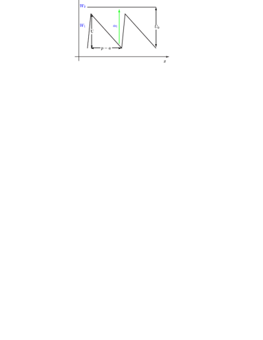
FIG. 1.: Model $(a)$: ratchet potential ($W_{1}$) and diffusive state $2$. The parameters are chosen so that $a/p=0.1$, $U=10kT,U_{0}=12kT,\omega/D=50$.

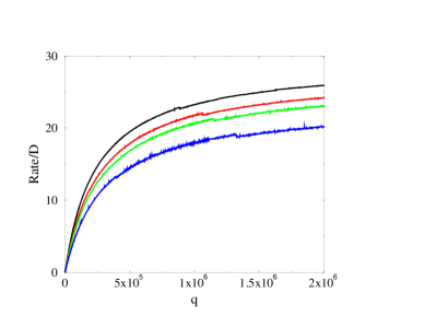
FIG. 2.: Results for the rate of ATP consumption for model $(a)$ with $\omega/D=50$ and various forces (top to bottom curves: $F_{ext}=0.0,-1.0,-3.0,-5.0$ in units of $kT/p$.

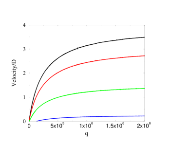
FIG. 3.: Results for the sliding velocity for model $(a)$ in units of $p$ with the same values of the forces as in fig.2.

REFERENCES

- [1] B. Alberts, D. Bray, J. Lewis, M.Raff, K. Roberts, and J.D. Watson. The Molecular Biology of the Cell. Garland, New York, 1994.
- [2] H.E. Huxley and W. Brown. J. Mol. Biol., 30:383–434, 1967.
- [3] A.F. Huxley. Prog. Biophys., 7:255, 1957.
- [4] T.L. Hill. Prog. Biophys. Mol. Biol., 28:267, 1974.
- [5] N. Thomas and R.A. Thornhill. J. Phys. D, 31:253–266, 1998.
- [6] A.F. Huxley and R.M. Simmons. Nature, 233:533–538, 1971.
- [7] S. Leibler and D.A. Huse. J. Cell Biol., 121:1357–1368, 1993.
- [8] A. Parmeggiani, F. Jülicher, A. Ajdari, and J.Prost. Phys. Rev. E, 60:2127–2140, 1999.
- [9] M.O. Magnasco. Phys. Rev. Lett., 71:1477–1481, 1993.
- [10] J. Prost, J.F. Chauwin, L. Peliti, and A. Ajdari. Phys. Rev. Lett., 72:2652–2655, 1994.
- [11] C.R. Doering, W. Horsthemke, and J. Riordan. Phys. Rev. Lett., 72:2984–2987, 1994.
- [12] F. Jülicher and J. Prost. Phys. Rev. Lett., 75:2618–2621, 1995.
- [13] I. Derényi and T. Vicsek. Phys. Rev. Lett., 75:374–377, 1995.
- [14] R.D. Astumian. Science, 276:917–922, 1997.
- [15] A.B. Kolomeisky and B. Widom. J. Stat. Phys., 93:633–645, 1998.
- [16] R.D. Vale and F. Oosawa. Adv. Biophys., 26:97–134, 1990.
- [17] R.P. Feynman, R.P. Leighton, and M. Sands. The Feynman Lectures on Physics. Addison–Wesley, Reading, MA, 1966.
- [18] F. Jülicher, A. Ajdari, and J. Prost. Rev. Mod. Phys., 69:1269–1281, 1997.
- [19] T. Duke and S. Leibler. Biophys. J., 71:1235–1247, 1996.
- [20] M. E. Fisher and A. B. Kolomeisky. Proc. Natl. Acad. Sci. USA, 96:6597–6602, 1999.
- [21] K. Visscher, M. J. Schnitzer, and S.M. Block. Nature, 400:184–189, 1999.
- [22] A. Fersht. Enzyme Structure and Mechanism. New York, Freeman, 1985.
- [23] We thank one of the referees for this observation.