Correlation versus mean-field contributions to excitons, multi-excitons, and charging energies in semiconductor quantum dots

Abstract

Single-dot spectroscopy is now able to resolve the energies of excitons, multi-excitons, and charging of semiconductor quantum dots with $\lesssim 1$ meV resolution. We discuss the physical content of these energies and show how they can be calculated via Quantum Monte Carlo (QMC) and Configuration Interaction (CI) methods. The spectroscopic energies have three pieces: (i) a “perturbative part” reflecting carrier-carrier direct and exchange Coulomb energies obtained from fixed single-particle orbitals, (ii) a “self-consistency correction” when the single particle orbitals are allowed to adjust to the presence of carrier-carrier interaction, and (iii) a “correlation correction.” We first apply the QMC and CI methods to a modle single-particle Hamiltonian: a spherical dot with a finite barrier and single-band effective mass. This allows us to test the convergence of the CI and to establish the relative importance of the three terms (i) – (iii) above. Next, we apply the CI method to a realistic single-particle Hamiltonian for a CdSe dot, including via a pseudopotential description the atomistic features, multi-band coupling, spin-orbit effects, and surface passivation. We include all bound states (up to 40,000 Slater determinants) in the CI expansion. Our study shows that: (1) typical exciton transition energies, which are $\sim 1$ eV, can be calculated to better than 95% by perturbation theory, with only a $\sim 2$ meV correlation correction; (2) typical electron addition energies are $\sim 40$ meV, of which correlation contributes very little ($\sim 1$ meV); (3) typical biexciton binding energies are positive and $\sim 10$ meV and almost entirely due to correlation energy, and exciton addition energies are $\sim 30$ meV with nearly all contribution due to correlation; (4) while QMC is currently limited to a single-band effective mass Hamiltonian, CI may be used with much more realistic models, which capture the correct symmetries and electronic structure of the dots, leading to qualitatively different predictions than effective mass models; and (5) and CI gives excited state energies necessary to identify some of the peaks that appear in single-dot photoluminescence spectra.

I Introduction: The physical content of exciton, multiexciton, and charging energies in dots

Small semiconductor dots, such as semiconductor embedded Stranski-Krastanow (SK) dots or “free-standing” colloidal dots, are engineered and studied for their optical and transport properties.Bimberg:1999 ; Woggon:1997 ; Jacak:1998 Measurements on these dots have centered around quantities such as excitons,Marzin:1994 ; Fafard:1995 ; Yang:2000 multi-excitons,Dekel:1998 ; Dekel:2000 ; Landin:1999 ; Toda:1999 ; Zrenner:2000 and charging energies.Fricke:1996 ; Tarucha:1996 ; Banin:1999 ; McEuen:1991 ; McEuen:1992 Advanced experimental techniques, such as single-dot spectroscopy, are able to resolve to such energies to $\lesssim 1$ meV resolution. This article discusses the physical content of such measured quantities in terms of the mean-field (direct and exchange) Coulomb energies, which are relatively simple to model, and correlation energies, which we calculate by two leading methods in the field — Quantum Monte Carlo (QMC) and Configuration-Interaction (CI).

Let us consider a quantum dot with $M$ holes in the valence band and $N$ electrons in the conduction band. The total energy of the dot is $E_{M,N}(\alpha)$, where $\alpha$ is a quantum number that identifies the state of the system. Only differences in energy are accessible to experiment. We focus on four physical quantities:

(i) Exciton energies.

The exciton transition energy $E_{X}^{(ij)}$ is the difference in total energy of a dot having as a dominant configuration an electron in level $e_{i}$ and a hole in level $h_{j}$ and a dot in the ground state,

$$E_{X}=E_{1,1}(e_{i}^{1},h_{j}^{1})-E_{0,0}.$$ (1)

Typical excitonic transition energies in III-V or II-VI dots, measured experimentallyFafard:1995 ; Bawendi:1990 by photoluminescence (PL) or by absorption, are 1 – 3 eV. The exciton binding energy $\Delta_{X}$ is the difference between the total energy of a system consisting of two infinitely separated identical dots, one with a hole in $h_{0}$ and the other with an electron in $e_{0}$, and the total energy of a quantum dot with an exciton:

$$\Delta_{X}=E_{1,0}+E_{0,1}-E_{1,1}-E_{0,0},$$ (2)

where $E_{1,0}$ stands for $E_{1,0}(h^{1}_{0}e^{0}_{0})$, $E_{0,1}=E_{0,1}(h^{0}_{0}e^{1}_{0})$, and $E_{1,1}=E_{1,1}(h^{1}_{0}e^{1}_{0})$. Typical exciton binding energies in III-V and II-VI dots are 10-200 meV.Fafard:1995 ; Bawendi:1990

(ii) Biexciton energies.

The biexciton binding energy $\Delta_{XX}$ is the difference between twice the exciton energy (or the energy of a system of two infinitely separated dots, each with an electron-hole pair), and the biexciton energy:

$$\Delta_{XX}=2E_{1,1}-E_{2,2}-E_{0,0}.$$ (3)

The biexciton binding energy is positive (“bound biexciton”) when the total energy of two excitons in the same dot is lower than the energy of the two excitons in two separate dots. A bound biexciton appears as a red-shifting of the exciton luminescence energy when a second exciton is present. This was seen in single-dot spectroscopy e. g. for InAs/GaAs.Dekel:1998 ; Dekel:2000 ; Zrenner:2000 ; Zrenner:1999 Biexciton binding energies in III-V dots are 1 – 6 meV.Zrenner:1999 ; Brunner:1994 ; Kuther:1998 ; Kamada:1998 ; Kulakovskii:1999 ; Gindele:1999

(iii) Multi-exciton energies.

The N-th exciton charging energy $W_{N}$ is the minimum energy needed to add to a dot having $N-1$ electron-hole pairs (excitons) in their ground state one additional exciton,

$$W_{N}=E_{N,N}-E_{N-1,N-1}.$$ (4)

Physically, $W_{N}$ is the highest possible energy for a photon emitted in the transition from the lowest energy state of $N$ excitons to a state with $N-1$ excitons. The difference in successive multi-exciton charging energies is the N-th exciton addition energy $\Delta^{(X)}_{N,N+1}$,

$$\begin{split}\Delta_{N,N+1}^{(X)}&=W_{N}^{(X)}-W_{N-1}^{(X)}\\ &=E_{N+1,N+1}+E_{N-1,N-1}-2E_{N,N}.\\ \end{split}$$ (5)

(iv) Electron loading energies.

The electron charging energy $\mu_{N}^{(e)}$ is the chemical potential needed to add an electron to a dot already having $N-1$ electrons:

$$\mu_{N}^{(e)}=E_{0,N}-E_{0,N-1},$$ (6)

whereas the electron addition energy is the difference between two successive chemical potentials,

$$\begin{split}\Delta_{N,N+1}^{(e)}&=\mu_{N}^{(e)}-\mu_{N-1}^{(e)}\\ &=E_{0,N+1}+E_{0,N-1}-2E_{0,N}.\\ \end{split}$$ (7)

Electron addition energies in colloidal dotsBanin:1999 are $\sim 200$ meV, whereas in SK dotsFricke:1996 ; Warburton:1998 they are $\sim 20$ meV.

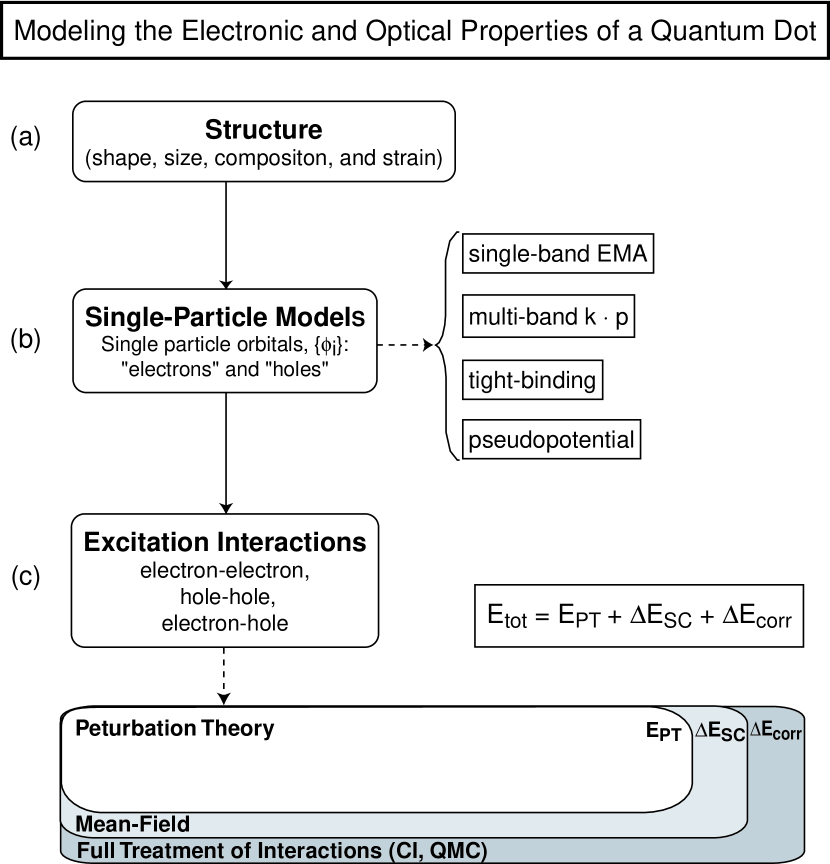
Figure 1: The three steps to modeling a quantum dot. (a) The structure is modeled by choosing a size, shape, and composition profile, and determining the strain. (b) Single particle properties of the electrons and holes are found by solving a Schrödinger equation for a chosen level of renormalization (EMA, $k\cdot p$, tight-binding, or pseudopotential). (c) Interactions between excitations (electron-electron, electron-hole, hole-hole) are added to the single particle model, using either perturbation theory $E_{\text{PT}}$; self-consistent mean-field theory, which adds the self-consistent contribution $\Delta E_{\text{SC}}$, or full treatment (CI or QMC), which adds the correlation energy $E_{\text{corr}}$.

The definitions given here in Eqs. (1)–(7) are operational, model-independent. A central question in the field is how to approximate these quantities through models. This requires knowing how much of the energy involved in the precesses described by Eqs. (1)–(7) are due to “mean-field” effects, which can be modeled relatively simply, and how much is due to inter-particle correlation, which is more intricate to model. Figure 1 illustrates the steps required to model the electronic and optical properties of a quantum dot: (a) choosing a structure (including size, shape, composition, and strain), (b) solving a single particle model, and (c) treating interactions among the electrons and holes. In this paper we are concerned with general trends in correlation in dots, so we focus mainly on the choice of single particle model, Fig. 1(b), and treatment of interactions, Fig. 1(c).

As illustrated in Fig. 1(b), the calculations of the quantities of Eqs. (1)–(7) require one to assume an underlying single-particle model, which determines the single particle states (conduction electrons and holes). The single-particle model is cast as a Schrödinger equation with an effective single-particle potential. This potential contain all structural information about the system: the size, shape, composition, surfaces, interfaces of the dot system. Various levels of renormalization exist for the quantum dot single-particle model. The simplest is an effective mass (“particle-in-a-box”) model, in which the electron and hole excitations come from single parabolic bands. Better approximations are the multi-band $k\cdot p$, tight-binding, and pseudopotentials.

The single-particle models do not usually contain the Coulomb interactions between the single-particle excitations (i. e. electron-electron, electron-hole, and hole-hole excitations). Instead, these interactions must be added to the model, as shown in Fig. 1(c). We classify the treatment of interaction among the single-particle excitations in three levels: (i) first order Perturbation Theory (PT),Dekel:1998 ; Barenco:1995 ; Franceschetti:1999 ; Franceschetti:2000a ; Franceschetti:2000b ; Williamson:2000c which includes direct and exchange Coulomb interactions, $J$ and $K$, evaluated from fixed single-particle orbitals; (ii) Self-Consistent Mean-Field (MF),Franceschetti:1997 in which the direct and exchange Coulomb terms are solved self-consistently [the difference between (ii) and (i) is called “self-consistency correction” $\Delta E^{\text{SC}}$]; and (iii) correlated methods, such as CIDekel:1998 ; Barenco:1995 ; Franceschetti:1999 ; Franceschetti:2000a ; Franceschetti:2000b ; Williamson:2000c or QMC,Harju:1999 ; Austin:1988 ; Bolton:1996 ; Shumway:1999 ; Pederiva:2000 ; Lee:1998a ; Luczak:2000 ; Mak:1998 ; Egger:1999a ; Egger:1999b ; Egger:1999c which include all many-body effects of interactions. The difference between the exact energy (iii) and the mean-field energy (ii) is called the “correlation correction,” $\Delta E^{\text{corr}}$. Thus, the energy for a dot with $M$ holes and $N$ electrons can be separated into three terms,

$$E_{M,N}^{\text{tot}}=E_{M,N}^{\text{PT}}+\Delta E_{M,N}^{\text{SC}}+\Delta E_{M,N}^{\text{corr}}$$ (8)

which are perturbation theory $E_{M,N}^{\text{PT}}$, self-consistent corrections $\Delta E_{M,N}^{\text{PT}}$, and the correlation correction $\Delta E_{M,N}^{\text{corr}}$.

Table 1: Relationship between the choice of single particle models for quantum dots and the availability of QMC and CI methods to calculate correlation energy [see Fig. 1, (b) and (c)]. This information motivates our approach to studying correlation: first we test the convergence of CI against QMC calculations using a simple single-band EMA model, then we present CI calculations on a realistic multi-band pseudopotential quantum dot model to illustrate features missed by the simple model.

Level of Renormalization	Model	CI	QMC
All electron	Exact Hamiltonian	no	no
Valence only	Multi-Band Pseudopotential	yes	no${}^{\text{b}}$
	Tight-binding	yes	no${}^{\text{b}}$
Active electron only	Multi-Band $k\cdot p$	yes	no
	Single-Band EMA	yes	yes

Due to computational limitations, the methods available to calculate correlation are dependent on which single-particle model is chosen (level of renormalization). The computational cost for accurately calculating correlation energies increases rapidly with the number of electrons one needs to consider. The number of electrons depends on both the dot’s size and on the type of renormalization one uses for the Hamiltonian. As summarized in Table 1, three levels of renormalization are pertinent:

(a) The all electron approach, where the number of electrons per atom equals its atomic number. Thus, Si has 14 electrons per atom, and a 40 Å diameter spherical Si dot has $1,600\times 14=22,400$  electrons. This is outside the reach of QMC, CI, and density functional methods.

(b) The valence-only pseudopotential approach, where the “core” electrons are removed as dynamic variables and replaced by an (often non-local) ionic potential. Thus, Si has 4 electrons per atom, and a 40 Å diameter spherical Si dot has $1,600\times 4=6,400$  electrons. This is outside the reach of density functional methods, and too large for QMC calculations, which are currently limited to about 25 Si atoms (100 electrons).Mitas:2000 Note that the all-valence pseudopotential approach can be further simplified, with no additional approximations by searching for eigensolutions in a fixed “energy window,”Wang:1994a ; Wang:1994c ; Wang:1996a e. g., near the band edges. Thus, a 40 Å diameter Si dot would require calculating $\sim 10$ eigensolutions. This trick makes pseudopotential calculations of dots feasible,Franceschetti:1999 ; Franceschetti:1997 ; Fu:1998a ; Wang:1998a ; Wang:2000a and CI may be used to compute correlation energies from the single particle solutions.Franceschetti:1999 ; Franceschetti:2000a ; Franceschetti:2000b ; Williamson:2000c It would be interesting if such folding techniques could be applied to QMC.

(c) The “active-electron-only” Effective Mass Approximation (EMA) approach, where all of the “indigenous” core and valence electrons are eliminated (replaced by dielectric screening) and only additional, band-edge electrons and holes are considered. Thus a 40 Å diameter Si dot has zero electrons. One can study added electrons and holes. This renormalization represents a severe approximation with respect to levels (a) and (b) above. Both QMC and CI methods may be readily applied to EMA Hamiltonians. Some improvement can be made by using several bands to describe the additional electrons and holes using the $k\cdot p$ formalism,Stier:1999 ; Grundmann:1995 but current QMC methods do not treat $k\cdot p$ Hamiltonians.

Most correlated calculations on quantum dots have used such a single-band effective mass model [level (c), above], where multi-band and inter-valley couplings are ignored. This particle-in-a-box description of the mean-field problem was recentlyFranceschetti:1999 ; Franceschetti:1997 ; Fu:1998a ; Wang:1998a ; Wang:2000a contrasted with the pseudopotential solution of the problem [(b) above] both for “free-standing” (colloidal) dots and for semiconductor-embedded SK dots. It was found that for “free-standing” dots (InP,Fu:1998a CdSeWang:1998a ) the effective mass approach can lead to energy shifts of the orderFu:1998a ; Wang:1998a $\sim 500$ meV; lead to reverse order of (s,p) levels;Fu:1998a miss more than half of the single-particle eigenvalues in a 0.5 eV energy range near the band edge;Wang:1998a underestimate the Coulomb integrals $J_{ij}$ [Eq. (II.1)] byFranceschetti:1997 $\sim 20\%$; and miss all the long-range part of the exchange integralsFranceschetti:1999 $K_{ij}$. For pyramidal SK dotsWang:2000a the errors are somewhat smaller: shifts in the energy levels for electrons and holes are $\sim 35$ meV and $\sim 110$ meV, respectively; energy spacings from EMA are about a factor of two too large; and the polarization ratio for dipole transitions along the two directions is 1 instead of 1.3. Such limitation in the EMA create a dilemma when modeling correlation as summarized in Table 1. On one hand CI expansions maybe applied to realistic single-particle models (e. g. pseudopotentials), but converge slowly with the number of configurations. On the other hand, QMC methods can give numerically exact answers including all correlation, but currently are limited to simple single-band effective mass models. This situation prompts us to use the following strategy to study correlation effects: First, we consider a simplified “particle-in-a-box” single-band EMA model which can be treated both via QMC and CI. Our best CI calculations for the EMA model include all bound states, but neglect continuum states. Second, we consider a CdSe dot whose single-particle properties are described realistically by pseudopotentials, and the correlation is treaded via CI only.

Table 2: Measurable quantities for our single-band spherical model dot, with effective masses $m_{e}=0.1$ and $m_{h}=0.5$, dielectric constant $\epsilon=12$, dot-material band gap $E_{\text{gap}}=1$ eV, and band offsets $\Delta E_{v}=200$ eV and $\Delta E_{c}=400$ meV. For each quantity we give the magnitude, the mean-field value, the correlation correction, and the percent of the energy recovered by CI expansion of using all bound states. All energies are given in meV, and electron charging and total energies are measured relative to the dot material CBM.

Quantity	Magnitude	Mean Field	Correlation	% CI
Exciton total energy, $E_{1,1}$ $(e_{0}^{1},h_{0}^{1})$	$1136.3$	$1138.3$	$2.0$	$100.1$
Biexciton total energy, $E_{2,2}$ $(e_{0}^{2}h_{0}^{2})$	$2266.5$	$2277.3$	$10.9$	$100.2$
Total energy of two electrons, $E_{0,2}$ $(e_{0}^{2})$	$335.0$	$335.8$	$0.8$	$100.1$
Exciton transition energy, $E_{X}$, [Eq. (1)]	$1136.3$	$1138.3$	$2.0$	$100.1$
Exciton binding energy, $\Delta_{X}$, [Eq. (2)]	$46.2$	$44.1$	$2.0$	$97.8$
Biexciton binding energy, $\Delta_{XX}$, [Eq. (3)]	$6.2$	$-0.6$	$6.8$	$64.5$
1st exciton charging energy, $W_{1}^{(X)}$, [Eq. (4)]	$1136.3$	$1138.3$	$2.0$	$100.1$
2nd exciton charging energy, $W_{2}^{(X)}$, [Eq. (4)]	$1130.1$	$1139.0$	$8.9$	$100.2$
1st exciton addition energy, $\Delta^{(X)}_{1,2}$, [Eq. (5)]	$-6.2$	$0.6$	$6.8$	$64.5$
1st electron charging energy, $\mu^{(e)}_{1}$, [Eq. (6)]	$147.5$	$147.5$	$0.0$	$100.0$
2nd electron charging energy, $\mu^{(e)}_{2}$, [Eq. (6)]	$187.5$	$188.3$	$0.8$	$100.1$
1st electron addition energy, $\Delta^{(e)}_{1,2}$, [Eq. (7)]	$40.0$	$40.8$	$0.8$	$101.4$

Our single-band EMA dot has been chosen to be representative of SK and colloidal dots. We summarize the properties of our model dot in Table 2. We find that for the single-band model dot:

(i) Typical exciton transition energies for our model dots are $\sim 1$ eV, and typical exciton binding energies are $\sim 50$ meV. Of this, MF gives $>95$% of the binding energy. Correlation is only $\sim 2$ meV, of which QMC provides an accurate solution Although CI misses half the correlation energy, i.e. $\sim 1$ meV, it still captures $\sim 98$% of the total binding energy.

(ii) Typical biexciton transition energies for our dots are $\sim 2$ eV and typical biexciton binding energies are $\sim 6$ meV. The biexciton binding energy from mean-field theory is slightly negative (unbound biexcitons), so the positive biexciton binding is in fact due to $\sim 6$ meV of correlation energy. QMC captures all the correlation energy, whereas our CI captures only half (about 4 meV), so that the CI estimate of biexciton binding is only about 65% of the true value.

(iii) Typical electron charing energies for our dots are $\mu_{1}^{(e)}\approx 150$ meV, relative to the dot material CBM, while addition energies are $\Delta_{1,2}^{(e)}\approx 40$ meV. Of this, correlation energy is very small ($\sim 1$ meV), so mean-field or even perturbation theory describes dot charging and addition energies very well.

For our realistic CdSe dot we find that CI can be effectively combined with accurate pseudopotential description of the MF problem, thus incorporating surface effects, hybridization, multi-band coupling. Furthermore, CI can calculate excited states easily, thus obtaining the many transitions seen experimentally, rather than only ground-state–to–ground-state decay calculated by conventional QMC (note, however, that extensions of QMC to several excited states are possibleCeperley:1988 ; Bernu:1990 ).

II Methods of Calculation

II.1 Uncorrelated methods: perturbation theory and mean field methods

The first-order perturbation energy $E_{M,N}^{PT}$ [Eq. (8)] can be written analytically as:

$$E_{M,N}^{PT}=E_{0,0}+(\sum_{c}\varepsilon_{c}-\sum_{v}\varepsilon_{v})+\sum_{v<v^{\prime}}(J_{v,v^{\prime}}-K_{v,v^{\prime}})+\sum_{c<c^{\prime}}(J_{c,c^{\prime}}-K_{c,c^{\prime}})-\sum_{v,c}(J_{v,c}-K_{v,c}),$$ (9)

where $\varepsilon_{i}$ are the single-particle energies, $J_{i,j}$ are the direct Coulomb energies, and $K_{i,j}$ are the exchange energies. The single-particle energies $\varepsilon_{i}$ are often obtained from the solution of an effective single-particle Schrödinger equation,

$$\{-\frac{1}{2}\nabla^{2}+V_{\text{eff}}\}\psi_{i}=\varepsilon_{i}\,\psi_{i}$$ (10)

where $V_{\text{eff}}$ is an effective potential. The Coulomb and exchange energies are given in terms of the single-particle wave functions $\psi_{i}$ by:

$$J_{i,j} = \int{|\psi_{i}({\bf r})|^{2}\,|\psi_{j}({\bf r}^{\prime})|^{2}\over\epsilon({\bf r},{\bf r}^{\prime})\,|{\bf r}-{\bf r}^{\prime}|}\,d{\bf r}\,d{\bf r}^{\prime}$$

$$K_{i,j} = \int{\psi_{i}^{*}({\bf r})\,\psi_{j}^{*}({\bf r})\,\psi_{i}({\bf r}^{\prime})\,\psi_{j}({\bf r}^{\prime})\over\epsilon({\bf r},{\bf r}^{\prime})\,|{\bf r}-{\bf r}^{\prime}|}\,d{\bf r}\,d{\bf r}^{\prime},$$ (11)

where $\epsilon$ is the dielectric constant of the quantum dot.

The self-consistent contribution $E^{\text{SC}}_{M,N}$, given by the first two terms on the right hand side of Eq. (8), arises from the self-consistent rearrangement of the single-particle wavefunction in respond to the electrostatic field, Eq. (II.1), generated by the excitation of electrons and holes.

II.2 The correlated, many-particle methods

II.2.1 Quantum Monte Carlo

The original QMC methodMcMillian:1965 was based on the variational technique, a simple, yet powerful theoretical tool. In a variational calculation, one proposes a parameterized trial wavefunction $\Psi_{T}^{\{\lambda\}}(R)$, where $\lambda$ represents a set of variational parameters and $R$ represents the coordinates of all the particles. The energy expectation value

$$E^{\{\lambda\}}_{T}=\frac{\int dR\Psi^{\{\lambda\}*}_{T}(R)H\Psi^{\{\lambda\}}_{T}(R)}{\int dR\Psi^{\{\lambda\}*}_{T}(R)\Psi^{\{\lambda\}}_{T}(R)},$$ (12)

may be minimized with respect to the variational parameters $\lambda$ to give an estimate for the ground state energy and ground state wavefunction. This integral may be evaluated analytically, or Monte Carlo integration may be used. In this simplest formulation, QMC is formally equivalent to the variational techniques commonly applied to excitons in nanostructures.Bastard:1988 Because the integral is over all electron and hole coordinates $R$, variational QMC calculations resemble classical simulations: a configuration of particle positions $R$ undergoes a random walk through configuration space, using the rules of Metropolis Monte Carlo integration. The sequence of configurations, $R_{i},R_{i+1},\ldots$, samples the density $|\Psi_{T}(R)|^{2}$.

The real power of QMC is that it can go beyond the variational formalism and actually project the true ground state energy from an input variational trial function, $\Psi_{T}$.Ceperley:1979 By weighting the the configuration as it samples configuration space, the random walk can identified with the imaginary time propagator $\exp(-H\tau)$. In this diffusion Monte Carlo algorithm,Ceperley:1979 ; Schmidt:1984 the random walk in configuration space actually samples $\Psi_{T}^{*}\Phi_{0}$ where $\Phi_{0}$ is the true ground state wavefunction. The energy expectation value along the walk $E_{0}=\langle\Psi_{T}|H|\Phi_{0}\rangle/\langle\Psi_{T}|\Phi_{0}\rangle$ is then the true ground state energy of the many-body Hamiltonian. That is, even though the true ground state wavefunction $\Phi_{0}$ is never explicitly calculated, its energy can be sampled from a random walk. In the remainder of the paper, the term QMC will refer to the diffusion Monte Carlo algorithm, unless explicitly noted otherwise.

Applications of QMC to quantum dots have used variational QMC,Harju:1999 diffusion QMC,Austin:1988 ; Bolton:1996 ; Shumway:1999 ; Pederiva:2000 ; Lee:1998a ; Luczak:2000 and a path-integral formulation, related to the diffusion algorithm and based on Feynman path integrals.Mak:1998 ; Egger:1999a ; Egger:1999b ; Egger:1999c Harju et alHarju:1999 have used both direct diagonalization and VMC to calculate the ground state energy of up to 6 electrons in a two-dimensional harmonically confined dot. Diffusion QMC within the EMA has been used (1) by AustinAustin:1988 to calculate the binding energy of excitons in a spherical dot as a function of dot radius, (2) by BoltonBolton:1996 to calculate the energy of up to 4 electrons in a two-dimensional harmonically confined dot in the presence of a magnetic field, (3) by Shumway et alShumway:1999 to calculate total energies for electron addition to a pyramidal dot, (4) by Pederiva et alPederiva:2000 to calculate ground and excitation energies for up to 13 electrons in a three-dimensional harmonically confined dot and compare to HF and LSDA, and (5) by Luczak et alLuczak:2000 to study energies of up to 20 electrons confined to a two-dimensional harmonic potential. Lee et alLee:1998a have used QMC within the EMA to study a pair of electrons in a two-dimensional parabolic confining potential. Path integral QMC has been used by Egger et alEgger:1999a to studied crossover from Fermi liquid to Wigner molecule behavior using PIMC within the EMA on up to 8 electrons in a two-dimensional harmonically confined dot, and by Harting et alHarting:2000 to calculate the total energy of up to 12 electrons in a two-dimensional harmonically confined dot.

II.2.2 Configuration Interaction

In the CI approach, the solutions of the many-body Hamiltonian are expanded in terms of Slater determinants $|\Phi\rangle$ obtained by removing $M$ electrons from the valence band and adding $N$ electrons to the conduction band:

$$|\Psi\rangle=\!\!\sum_{h_{1}\ldots h_{M}}\!\sum_{\phantom{h}e_{1}\ldots e_{N}}\!\!A(h_{1}\ldots h_{M},e_{1}\ldots e_{N})|\Phi_{h_{1}\ldots h_{M},e_{1}\ldots e_{N}}\rangle,$$ (13)

where:

$$|\Phi_{h_{1}\ldots h_{M},e_{1}\ldots e_{N}}\rangle=d^{\dagger}_{h_{1}}\cdots d^{\dagger}_{h_{M}}c^{\dagger}_{e_{1}}\cdots c^{\dagger}_{e_{N}}\,|\Phi_{0}\rangle.$$ (14)

Here $d^{\dagger}_{h_{1}}\cdots d^{\dagger}_{h_{M}}$ create holes in the valence-band states $h_{1}\ldots h_{M}$, while $c^{\dagger}_{e_{1}}\cdots c^{\dagger}_{e_{N}}$ create electrons in the conduction band states $e_{1}\ldots e_{N}$. The Hamiltonian is then diagonalized in the basis of Slater determinants $|\Phi\rangle$. This approach gives access to not only the ground state of the system, but also excited states.

Full CI (FCI) includes all possible determinants from a given (finite) set of single particle basis functions, i. e. $N_{h}$ hole orbitals and $N_{e}$ electron orbitals. In the limit of an infinite set of basis functions, $(N_{h},N_{e})\rightarrow(\infty,\infty)$, FCI provides the exact many-body solution, which is equivalent to the QMC results. However, most CI applications use a small and finite basis set to solve the Schrödinger problem. Thus, even including in the CI expansion all possible Slater determinants from a finite number of single-particle states (FCI) does not provide an exact solution, in contrast to QMC. For our calculations we also only use a small, finite basis set of bound states, denoted $(N_{h},N_{e})$, therefore ground state total energies from FCI will be above the true ground state total energy. A useful truncated CI basis is Singles and Doubles Configuration Interaction (SDCI), which the set of all determinants obtained by exciting at most two particles (electrons or holes) from the ground-state (or reference) determinant. SDCI is equivalent to FCI for a single exciton (or two electrons), but is an approximation for two or more excitons (or three or more electrons).

The CI method has been used in the past to solve the the many-body Schrödinger equation in the EMA approximationLandin:1999 ; Barenco:1995 ; Hawrylak:1999 ; Hawrylak:2000a ; Hawrylak:2000b ; Brasken:2000 and also tight binding.Dib:1999 More recently, the CI approach has been used in the context of the empirical pseudopotential method (EPM) for single excitons,Franceschetti:1999 electron and hole addition energies,Franceschetti:2000a ; Franceschetti:2000b and multiexcitons.Williamson:2000c

III Application of QMC and CI to a single-band effective-mass dot with finite barrier

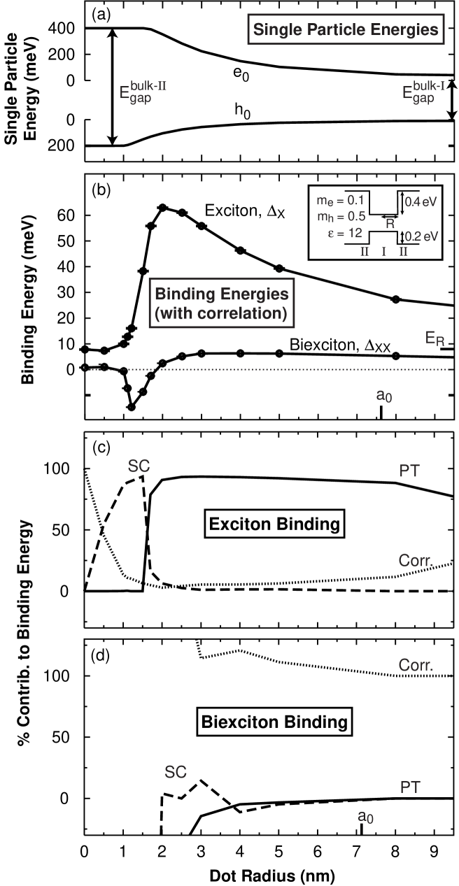
Figure 2: Exciton and biexciton binding energy versus dot radius as calculated by QMC, for the dot geometry shown in the inset. Panel (a) shows the energies of the non-interacting electron and hole band edge states. Panel (b) shows the the exciton binding energy $\Delta_{X}$ [Eq. (2)], and biexciton binding energy $\Delta_{XX}$ [Eq. (3)]. The bulk exciton Rydberg energy and Bohr radius are denoted $a_{0}=7.6$ nm and $E_{R}=7.9$ meV, respectively. Contributions to exciton and biexciton binding energy versus dot radius are shown in (c) and (d), respectively. Contributions are from: first order perturbation theory (PT), self-consistency correction (SC), and correlation (Corr.).

We first use a simplified single-band EMA model which can be treated by both QMC and CI. Our reference system is a spherical dot with radius $R=40$ Å, effective masses $m_{e}=0.1$ and $m_{h}=0.5$, dielectric constant $\epsilon=12$, and barriers $\Delta E_{\text{v}}=0.4$ eV and $\Delta E_{\text{c}}=0.2$ eV. The energies of the optical and electronic properties of this dot are summarized in Table 2. We have then varied the radius from 0 to 80 Å, while keeping the barriers fixed. This yields a range of bound electron and hole states. The energies of the lowest (i. e. band-edge) states $e_{0}$ and $h_{0}$ as a function of dot radius $R$ are shown in Fig. 2(a). When the radius $R$ of the dot goes to infinity we have a 3D bulk material called “material I” with $m_{e}=0.1$, $m_{h}=0.5$, and $\epsilon=12$. When the radius $R$ of the dot goes to zero we have a 3D bulk material called “material II” with $m_{e}$, $m_{h}$, and $\epsilon$ identical to “material I.” The band offsets between the two materials $\Delta E_{h}=0.2$ eV for the valence band and $\Delta E_{e}=0.4$ eV for the conduction band, so that the band-gap of “material II” is $\Delta E_{h}+\Delta E_{e}=0.6$ eV larger than the band-gap of “material I.” The bulk exciton in both materials is the same, and has a radius $a_{0}=76.2$ Å, a binding energy $E_{R}=7.873$ meV. Both bulk materials have a bound biexciton with the same binding energy, $\Delta^{\text{bulk}}_{XX}=0.716$ meV $=0.9E_{R}$, (calculated by QMC). In some calculations we have varied the barrier energy from $\Delta E_{\text{v}}=0.05$ eV to $\Delta E_{\text{v}}=4$ eV and $\Delta E_{\text{c}}=0.025$ eV to $\Delta E_{\text{c}}=2$ eV, while keeping the radius fixed at 40 Å. Our model system has thus been chosen to roughly capture some properties of small SK or colloidal dots, as summarized in Table 2.

III.1 Total energies for occupation by an exciton, biexciton, and two-electrons

Figure 3: CI convergence of the total energy for three cases: (a) an exciton, (b) a biexciton, and (c) two electrons. All energies are measured relative to the center of dot gap. For our CI expansion, we have used single and double substitutions (SDCI) and also all possible determinants (FCI). Note that SDCI is equivalent to FCI for cases (a) and (c). SDCI gives a good approximation to FCI for case (b), and involves far fewer determinants (see Table 3). In all cases our CI expansion captures about half of the correlation energy. The correlation energy (and hence CI error) is a very small fraction ($<1$%) of the total energy in all three cases.

Table 3: Number of determinants used for each of the CI calculations shown in Figs. 3 and 4, using only single and double substitutions (SDCI), or all possible slater determinants (FCI). Note that SDCI is equivalent to FCI for the case of an exciton or two electrons. For FCI the number of CI determinants for $M$ holes and $N$ electrons occupying $N_{h}$ hole states and $N_{e}$ electron states is $C_{M}^{2N_{h}}\cdot C_{N}^{2N_{e}}$.

		# of determinants
System	($N_{h}$,$N_{e}$)	SDCI	FCI
Exciton $(h^{1}e^{1})$:
	(1,1)	4	4
	(4,1)	16	16
	(4,4)	64	64
	(9,4)	144	144
	(10,4)	160	160
	(17,4)	262	262
	(20,4)	320	320
Biexciton $(h^{2}e^{2})$:
	(1,1)	1	1
	(4,1)	28	28
	(4,4)	199	784
	(9,4)	564	4284
	(10,4)	649	5320
	(17,4)	1356	15708
	(20,4)	1719	21840
Two Electrons$(h^{0}e^{2})$:
	(0,1)	4	4
	(0,4)	28	28
	(0,5)	153	153
	(0,10)	190	190

Figure 3 shows the total energy for (a) exciton, $E_{1,1}(e_{0}^{1},h_{0}^{1})$; (b) biexciton, $E_{2,2}(e_{0}^{2},h_{0}^{2})$; and (c) two-electrons, $E_{2,0}(e_{0}^{2},h_{0}^{0})$. We have decomposed the total energies into the three parts listed in Eq. (8): first-order perturbation theory ($E_{\text{PT}}$), self-consistent mean field ($E_{\text{PT}}+\Delta E_{\text{SC}}$), and the exact QMC result ($E_{\text{tot}}=E_{\text{PT}}+\Delta E_{\text{SC}}+\Delta E_{\text{corr}}$). We then plot the results of CI calculations as a function of the number of single-particle states $(N_{h},N_{e})$ used to generate the CI basis set, taking either singles and doubles only (SDCI) or all possible determinants (FCI). The CI energies for one determinant are equivalent to the MF result, and the FCI values must reach the QMC result in the limit of an infinite basis. The total number of CI determinants for $M$ holes and $N$ electrons occupying $N_{h}$ hole states and $N_{e}$ electron states is $C_{M}^{2N_{h}}\cdot C_{N}^{2N_{e}}$, where $C_{m}^{n}=n!/[m!(n-m)!]$. The factors of 2 are due to the spin-degeneracy of the single particle states. Table 3 lists the actual number of determinants for each of the FCI and SDCI data points in Fig. 3. The first three lines of Table 2 give a summary of the role of correlation energy and CI convergence in the total energy of these three systems.

In each system, the total energy estimated by first-order perturbation theory is above the true ground state energy (as required by the variational principle). Self-consistency improves upon first-order perturbation theory, and correlation provides additional improvement. For excitons, the self-consistency decreases the energy by $\sim 1$ meV, and correlation gives another $\sim 2$ meV improvement. The total energy, however, is $E_{1,1}=1136$ meV.  So, although our CI only recovers about half of the correlation energy, the total energy is only overestimated by about 0.1%. For the case of a biexciton, self-consistency also lowers the energy by $\sim 2$ meV, while correlation lowers the energy by another $\sim 10$ meV.  In calculations on a strain induced dot, Braskén et alBrasken:2000 found that SDCI captured $\gtrsim 90\%$ of the correlation energy for multi-excitons, based on comparison to FCI for one to four excitons. In our biexciton calculations, we also find that SDCI recovers nearly as much correlation energy as FCI, but this represents only about about half of the total correlation energy. Again, though, correlation represents a small part of the total energy of the biexciton, so CI (FCI and SDCI) only overestimate the total energy by $\sim 0.2$%. For a dot containing two electrons, corrections beyond first-order perturbation theory are much smaller, $\sim 1$ meV.   In fact, for the system calculated here, we find only a 0.35 meV decrease in the two-electron system with self-consistency, and correlation decreases the total energy by about another 0.8 meV.   Our CI expansion again captures about half this correlation energy, leading to negligibly small overestimation of the total energy ($<0.1$%).

III.2 Exciton and biexciton transition and binding energies

Measured quantities such as the exciton and biexciton binding energies represent differences between total energies. Even if the mean-field contributions dominate total energies, the mean-field contributions to differences of total energies may have significant contributions from correlation. Lines 4-6 of Table 2 summarize the role of correlation and CI convergence for the exciton transition energy, $E_{X}$ [Eq. (1)]; exciton binding energy, $\Delta_{X}$ [Eq. (2)]; and the biexciton binding energy, $\Delta_{XX}$ [Eq. (3)]. Correlation is only a small part (2 meV) of the exciton transition energy $E_{X}=1136.3$ meV.   So, even though our underconverged CI fails to capture all the correlation energy, $E_{X}$ is only overestimated by 0.1%. The same 2 meV of correlation energy is a much larger component of the exciton binding energy, $\Delta_{X}=46.2$ meV, so errors due to underconvergence of CI are more significant, and CI underestimates $\Delta_{X}$ by more than 2%. The biexciton binding energy $\Delta_{XX}=6.2$ meV is due entirely to 6.8 meV of correlation energy, so CI underconvergence is much more serious. Our CI calculation of biexciton binding is only 65% of the exact QMC result.

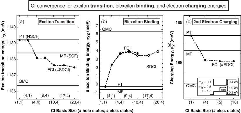
Figure 4: CI convergence of: (a) exciton transition energy, $E_{X}$ [Eq. (1)]; (b) biexciton binding energy, $\Delta_{XX}$ [Eq. (3)]; and (c) second electron addition energy, $\mu^{(e)}_{2}$ [Eq. (6)]. For our CI expansion, we have used single and double substitutions (SDCI) and also all possible determinants (FCI). Note that SDCI is equivalent to FCI for cases (a) and (c). SDCI gives a good approximation to FCI for case (b), and involves far fewer determinants (see Table 3). In all cases our CI expansion captures about half of the correlation energy. The correlation energy (and hence CI error) is a significant fraction of the the total energy only for case (b), biexciton binding.

In Fig. 4 we show the results of first-order perturbation theory ($E_{\text{PT}}$), self-consistent mean field ($E_{\text{PT}}+\Delta E_{\text{SC}}$), the exact QMC result ($E_{\text{tot}}=E_{\text{PT}}+\Delta E_{\text{SC}}+\Delta E_{\text{corr}}$), and CI convergence vs. basis size for (a) the exciton transition energy and (b) the biexciton binding energy. For the exciton transition energy, Fig. 4(a), increasing the CI basis does improve the calculated energy, but it is only a difference of $\sim 2$ meV out of a much larger exciton transition energy of 1.136 eV. On the other hand, the CI correction is essential to even approximate the biexciton binding energy, shown in Fig. 4(b). Note that the improvement of the biexciton binding with CI basis size is not monotonic. This is because the biexciton binding is a difference of one- and two-exciton energies. As the basis is increased, the relative improvement in the one- and two-exciton total energies varies, thus the calculated biexciton binding energy can actually decrease when the CI basis is improved. We also show the results of SDCI in Fig. 4(b).

III.2.1 Dependence on dot size

We have varied the dot radius from $R=0$ to $R=80$ Å, all in the strongly confined regime, $R\lesssim a_{0}=76.2$ Å. Figure 2(b) shows the exciton and biexciton binding energies as calculated by QMC. Figures 2(c) and 2(d) decompose the contributions to the exciton and biexciton binding into (1) first order perturbation theory, (2) self-consistency corrections, and (3) correlation corrections, as in Eq. (8).

The small $R$ limit is the energy of a bulk-II material, and all excitonic binding energy is from correlation. As the radius of the dot increases, the bulk-II exciton binds to the dot, the exciton binding energy is enhanced, and most of the binding energy comes from perturbation theory. The maximum in the binding energy occurs when the electron and hole are both individually bound to the dot, but the radius is small, so that the direct Coulomb interaction (from first order perturbation theory) is the strongest. The exciton binding energy exhibits a clear peak at around $R\approx 40$ Å, in similarity with previous calculations by Austin.Austin:1988 As the dot becomes larger, the direct Coulomb interaction from perturbation theory decreases, causing a decrease in the exciton binding energy. Finally, as the dot becomes comparable in size to the bulk-I exciton radius, correlation begins to have significant contributions to exciton binding. In the limit $R\gg a_{0}$ (not shown), the binding energy becomes that of a bulk-I exciton.

The biexciton binding energy is greatly enhanced in a quantum dot, except for the case of a very small dot with only a single weakly bound exciton. We find that the biexciton binding energy is remarkably insensitive to dot radius, having a value $\Delta_{XX}$ between 5.1 meV and 6.2 meV ($0.7~{}E_{R}$ to $0.9~{}E_{R}$) for dots with radii R between 2 nm and 8 nm ($0.3~{}a_{0}$ and $1.1~{}a_{0}$). This is in contrast the exciton binding energy, $\Delta_{X}$, which exhibits a clear peak at small dot radius. The size range $10\lesssim R\lesssim 18$ Å has a negative biexciton binding. Physically, these are small dots that can weakly bind two excitons, but with a higher total energy than separating the two excitons on two non-interacting, identical dots. We see from Fig. 2(d) that the biexciton binding energy is almost entirely due to correlation, as noted before.

III.2.2 Dependence on barrier height

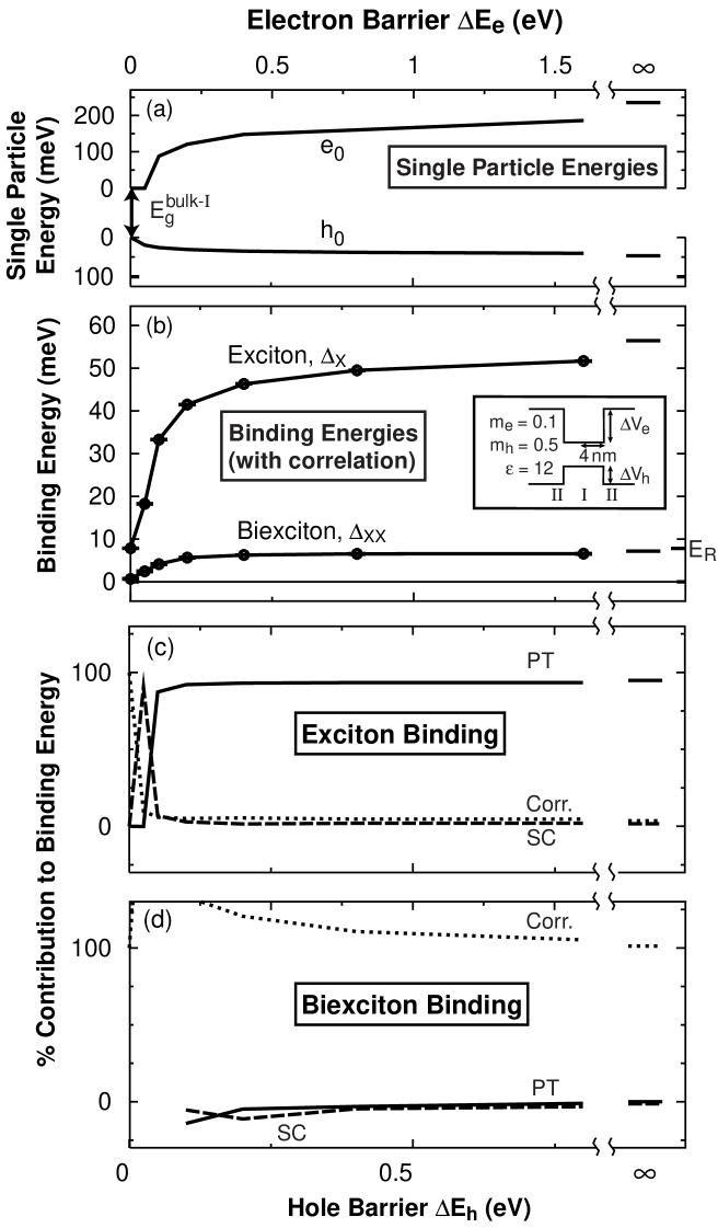
Figure 5: Exciton and biexciton binding energy (including correlation) as calculated by QMC as a function of versus barrier energy, with the constraint $\Delta E_{e}/\Delta E_{h}=2$, for the dot geometry shown in the inset. Panel (a) shows the single-particle energies of the non-interacting electron and hole band edge states. Panel (b) shows the the exciton binding energy $\Delta_{X}$ [Eq. (2)] and biexciton binding energy $\Delta_{XX}$ [Eq. (3)]. The bulk exciton Rydberg energy is denoted $E_{R}=7.9$ meV. Contributions to exciton and biexciton binding energy versus barrier energy are shown (c) and (d), respectively. Contributions are from: first order perturbation theory (PT), self-consistency correction (SC), and correlation (Corr.).

To study the effect of finite confining barriers on exciton and biexciton binding energies, we have varied the dot barriers from zero to infinity. In all calculations we have kept $\Delta E_{e}/\Delta E_{h}=2$ and used a radius of 40 Å. In Fig. 5(b) we plot the binding energies of excitons and biexcitons calculated with QMC as a function of barrier height. The 40 Å dot is able to bind an electron once $\Delta E_{e}\gtrsim 30$ meV, and binds a hole once $\Delta E_{h}\gtrsim 5$ meV. Unlike the behavior seen with varying the dot radius, increasing the confining potential leads to a monotonic increase in exciton and biexciton binding energies. For zero barrier potential, the exciton has the bulk-I exciton binding energy, $\Delta_{X}=E_{R}^{(I)}=7.9$ meV. As the barrier potential is increased enough to bind both electrons and holes, the exciton binding increases rapidly. The binding energy reaches a maximum of $\Delta_{X}=55~{}\text{meV}=7E_{R}$ for infinite barriers. Similarly, the biexciton binding energy starts from the bulk biexciton binding energy $\Delta_{XX}=0.7~{}\text{meV}=0.1E_{R}$ and increases to a maximum of $\Delta_{XX}=7.2~{}\text{meV}=1.0E_{R}$ for infinite barriers. Figures 5(c) and 5(d) show the contributions of perturbation theory, self-consistency correction, and correlation to the exciton and biexciton binding energy. Except for very weakly confined dots, the exciton is very well described by first-order perturbation theory. For weak confinement, the electron is unable to bind, but self-consistent interaction with the hole is able to bind the electron, so that the exciton binding energy is almost entirely due to self-consistency. For the weakest confinement, neither the electron nor the hole is bound, and the excitonic binding is entirely due to correlation. Again, biexciton binding is due entirely to correlation.

III.3 Multi-exciton energies

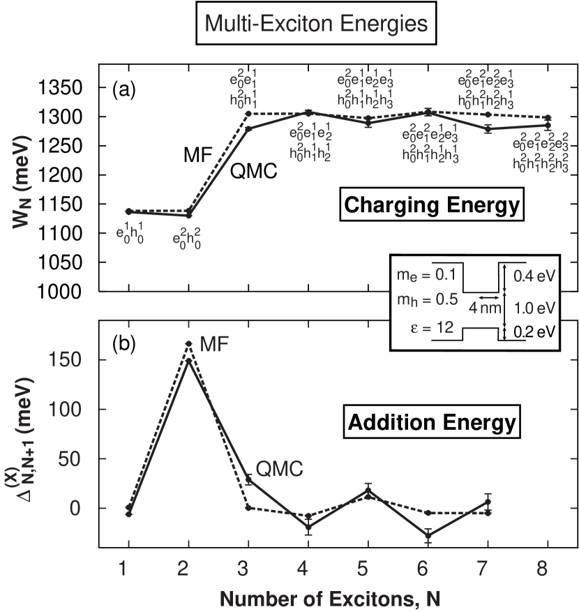
Figure 6: (a) Exciton charging [Eq. (4)], and (b) addition energies [Eq. (5)], for the dot shown in the inset. Because excitons are neutral, it is energetically favorable for a dot to hold many excitons.

Figure 6 shows mean-field and exact (QMC) results for the multi-exciton charging energies $W_{N}$ [Eq. (4)], and the multi-exciton additions energies, $\Delta^{(X)}_{N,N+1}$ [Eq. (5)]. The most prominent feature is the jump in the charging energy for $W_{3}$, which also appears as a peak in the addition energy $\Delta^{(X)}_{2,3}$. This “shell effect” arises because only the first two excitons can occupy the lowest energy $e_{0}$ and $h_{0}$ states. Starting with the third exciton, Pauli exclusion requires the addition excitons to start filling the next energy shell, $e_{1}h_{1}$ through $e_{3}h_{3}$. This is a feature of the single particle model, and does not require any treatment of correlation. Correlation is necessary to describe the decrease in charging energy for the second exciton, $W_{2}<W_{1}$, or equivalently the negative value of the first exciton addition energy $\Delta^{(X)}_{1,2}=-6.2$ meV. This is the positive biexciton binding energy $\Delta_{XX}=6.2$ meV, discussed earlier. As shown in lines 7-9 of Table 2, the correlation contribution for the second charging energy $W_{2}$ is 8.9 meV, considerably larger than the 2.0 meV for $W_{1}$. Our CI only captures about half the correlation energy, so it slightly overestimates the exciton charing energies, and considerably underestimates the negative value of $\Delta^{(X)}_{1,2}$.

III.4 Electron loading energies

Figure 7: (a) Electron charging energies [Eq. (6)], and (b) addition energies [Eq. (7)], for the dot shown in the inset. This dot can only hold up to four electrons, due to Coulomb repulsion. The conduction band minimum energy of the barrier material, $\Delta E_{e}=400$ meV is shown in panel (a).

Figure 7 shows mean-field and exact (QMC) results for electron charging energies $\mu_{N}$, [Eq. (6)], and the electron additions energies, $\Delta^{(e)}_{N,N+1}$ [Eq. (7)]. Because electrons are charged, Coulomb repulsion quickly limits the number of electrons that can be loaded into the dot. For our model, shown in the inset to Fig. 7, it is only energetically favorable to add four electrons; beyond this, electrons would rather escape into the barrier material conduction band, shown as a dashed horizontal line in Fig. 7(a). There is a peak in the electron addition energy $\Delta^{e}_{2,3}$ in Fig. 7(b). This is due the filling of the $e_{0}$ state by a spin-up and spin down electron (another “shell effect”). Both QMC and MF capture this single particle effect. As shown in Fig 4(c), our CI expansion recovers about half of the correlation energy for two electrons. However, the correlation energy in a two-electron dot is only about 1 meV, so CI errors are a negligible 0.5 meV. The small value of correlation and the good agreement of our CI calculations for dot charging are summarized in last three lines of Table 2

IV Application of CI to a multi-band dot described via plane-wave pseudopotentials

QMC calculations are currently limited to either small systems containing up to a few hundreds of electrons,Mitas:2000 ; Kent:1999 ; Torelli:2000 or to highly simplified model Hamiltonians (such as the EMA). A more accurate description of the electronic structure (Fig. 1) of semiconductor quantum dots can be obtained using the pseudopotential approach.Wang:2000a Unfortunately, QMC methods are presently unable to deal with the large number of electrons of a typical quantum dot, and CI is the only viable approach to treat correlation effects in large quantum dots described by atomistic pseudopotentials. In addition, the diagonalization of the CI Hamiltonian gives access to the excited states (unavailable in ground-state QMC calculations) as well as the ground state of the electronic system, thus enabling the calculation of the optical spectrum of quantum dots.

In order to illustrate the capabilities of the CI approach combined with a pseudopotential description of the electronic structure, we consider a nearly spherical CdSe quantum dot having the wurtzite lattice structure and a diameter of 38.5 Å. The surface dangling bonds are fully passivated using ligand-like atoms.Wang:1998a This quantum dot is representative of CdSe nanocrystals grown by colloidal chemistry methods.

We consider here only low-energy excitations of the electronic system, which are obtained by promoting electrons from states near the top of the valence band to states near the bottom of the conduction band. The band-edge solutions of Eq. (10) can be efficiently obtained using the folded spectrum method,Wang:1994a ; Wang:1994c ; Wang:1996a which allows one to calculate selected eigenstates of the Schrödinger equation with a computational cost that scales only linearly with the size of the system. In this approach, Eq. (10) is replaced by the folded-spectrum equation

$$\left[-\nabla^{2}+V_{ps}({\bf r})+{\hat{V}}_{NL}-\varepsilon_{ref}\right]^{2}\psi_{i}({\bf r},\sigma)=(\varepsilon^{0}_{i}-\varepsilon_{ref})^{2}\;\psi_{i}({\bf r},\sigma)\,,$$ (15)

where $\varepsilon_{ref}$ is an arbitrary reference energy. The lowest energy eigenstate of Eq. (15) coincides with the solution of the Schrödinger equation [Eq. (10)] whose energy is closest to the reference energy $\varepsilon_{ref}$. Therefore, by choosing the reference energy in the band gap, the band edge states can be obtained by minimizing the functional $A[\psi]=\langle\psi|({\hat{H}}-\varepsilon_{ref})^{2}|\psi\rangle$.

The solution of Eq. (15) is performed by expanding the wave functions $\psi_{i}({\bf r},\sigma)$ in a plane-wave basis set. To this purpose, the total pseudopotential $V_{ps}({\bf r})$ is defined in a periodically repeated supercell $\Omega$ containing the quantum dot and a portion of the surrounding material. The supercell $\Omega$ is sufficiently large to ensure that the solutions of Eq. (15) are converged within 1 meV. The single-particle wave functions can then be expanded as $\psi_{i}({\bf r},\sigma)=\sum_{\bf G}\,c_{i}({\bf G},\sigma)\,\exp(i{\bf G}\cdot{\bf r})$, where the sum runs over the reciprocal lattice vectors ${\bf G}$ of the supercell $\Omega$. The energy cutoff of the plane-wave expansion is the same used to fit the bulk electronic structure, to ensure that the band-structure consistently approaches the bulk limit. The minimization of the functional $A[\psi]$ is carried out in the plane-wave basis set using a preconditioned conjugate-gradients algorithm.

In the next step we construct a set of Slater determinants $|\Phi_{h_{1}\cdots h_{N},e_{1}\cdots e_{N}}\rangle$ [see Eq. (14)] obtained by creating $N$ holes in the valence band and $N$ electrons in the conduction band, and diagonalize the CI Hamiltonian in this basis set. Using the CI approach, we have calculated the multiexciton spectrum of a CdSe dot. We consider here up to three excitons and we use a CI basis set of 480 configurations for the single exciton, 43890 configurations for the biexciton, and 20384 configurations for the tri-exciton. All the relevant interactions (including electron-hole exchange) are included in the CI calculations. We assume that when an $N$-exciton is created in the quantum dot, it relaxes non-radiatively to the ground state before decaying radiatively into an $(N-1)$-exciton.

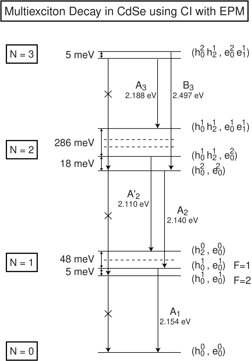
Figure 8: Schematic illustration of the leading contributions to peaks ($A_{3},B_{3},A^{\prime}_{2},A_{2},A_{1}$) appearing in Fig. 9. Solid horizontal lines are energies of $N=0$ to $N=4$ excitons, with dashed lines indicating states that do not participate in dipole transitions.

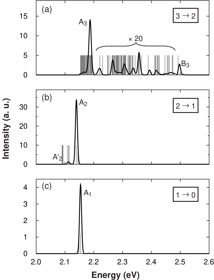
Figure 9: Exciton transition energies for a CdSe dot for (a) decay from three to two excitons, (b) decay from two to one excitons, and (c) decay of a single exciton. The intensity scale is different in each of the three panels, and weak transitions between peaks $A_{3}$ and $B_{3}$ in (a) have been magnified by $\times 20$. Grey vertical lines indicate all calculated transition energies, and solid black lines in the Gaussian broadened transitions weighted by calculated dipole transition strengths.

The calculated multiplet levels are shown in Fig. 8 and the emission spectrum is shown in Fig. 9. The three panels of Fig. 9 correspond to the recombination of (a) a tri-exciton into a biexciton ($3\rightarrow 2$), (b) a biexciton into a single-exciton ($2\rightarrow 1$), and (c) a single-exciton into the ground state ($1\rightarrow 0$), respectively. We assume that the low-energy states of the $N$-exciton are thermally populated ($kT=5\;{\rm meV}$) before recombination. We see from Fig. 9 that:

(i) The single-exciton recombination spectrum, Fig. 9(a), shows a single peak ($A_{1}$) centered at $2.154\;{\rm eV}$. It is well known Nirmal:1995 that in CdSe nanocrystals the electron-hole exchange interaction splits the lowest-energy excitonic state ($h_{0}^{1},e_{0}^{1}$) into two doublets, having total angular momentum $F=2$ and $F=1$ respectively (see Fig. 8 ). The lower-energy doublet ($F=2$) is optically forbidden, while the higher-energy doublet ($F=1$) is optically allowed. We find an energy separation of $\sim 5\;{\rm meV}$ between the two doublets. The emission peak $A_{1}$ observed in Fig. 9 comes from the recombination of the higher-energy doublet, which is thermally populated. This explains the relatively weak intensity of the single-exciton peak.

(ii) The biexciton recombination spectrum, Fig. 9(b), shows a strong peak ($A_{2}$) centered at $2.140\;{\rm eV}$. This peak originates from the recombination of a biexciton in the ground state ($h_{0}^{2},e_{0}^{2}$) into a single exciton in the $F=1$ state. The weak shoulder to the red of the main peak ($A^{\prime}_{2}$) is due to the recombination of a thermally occupied higher-energy biexciton state in the configuration ($h_{0}^{1}h_{2}^{1},e_{0}^{2}$). Note that several transitions from the biexciton ground state to single-exciton excited states are in principle possible, but have very weak oscillator strength. These transitions would occur to the red of the fundamental transition. The calculated biexciton binding energy is $2E_{X}-E_{XX}\sim 4\;{\rm meV}$. This value is probably underestimated due to the under-convergence of the CI expansion. Interestingly, the “apparent” biexciton binding energy, i.e. the red-shift of the main biexciton peak $A_{2}$ with respect to the single-exciton peak $A_{1}$, is $\sim 14\;{\rm meV}$ (not $4\;{\rm meV}$). The reason is that the biexciton recombination takes the quantum dot in the $F=1$ excited state, rather than the $F=2$ ground state (see Fig. 8). Thus we have $E(A_{1})-E(A_{2})=(E_{X}^{F=1}-E_{0,0})-(E_{XX}-E_{X}^{F=1})=\Delta_{XX}+2\,(E_{X}^{F=1}-E_{X}^{F=2})=4+2\times 5\;{\rm meV}=14\;{\rm meV}$.

(iii) In the case of three excitons we find that the ground state wave function originates primarily from the non-Aufbau configuration $h_{0}^{2}h_{2}^{1};e_{0}^{2}e_{1}^{1}$. In fact, the third hole prefers to occupy the $p$-like $h_{2}$ state rather than the $s$-like $h_{1}$ state, due to reduced Coulomb repulsion with the remaining two holes. Two main transitions are possible from the three-exciton ground state: the $e_{0}\rightarrow h_{0}$ recombination, which leaves the system into the excited biexciton configuration $h_{0}^{1}h_{2}^{1};e_{0}^{1}e_{1}^{1}$, leads to peak $A_{3}$ located at $2.188\;{\rm eV}$. The $e_{1}\rightarrow h_{2}$ recombination, which takes the system into the ground-state biexciton configuration $h_{0}^{2};e_{0}^{2}$, is responsible for peak $B_{3}$ centered at $2.497\;{\rm eV}$. Note that the $B_{3}$ transition originates from an exchange-split tri-exciton state (see Fig. 8) which is thermally populated, hence the relatively weak oscillator strength of the $B_{3}$ transition.

Note that a calculation considering only ground-state to ground-state transitions would miss most of the peaks observed in Fig. 9. The capability of the CI expansion to access excited states, coupled with the possibility of using a multi-band pseudopotential Hamiltonian for the calculation of the single-particle energies and wave functions, makes it the method of choice for calculating excited states of semiconductor quantum dots.

V Conclusion

We have studied the effects of correlation on a simplified, single-band model dot using both QMC and CI, and have studied correlation in the multi-exciton PL spectra of a realistically modeled CdSe dot using CI. Our results for the simplified, single band model are summarized in Table 2. We find the following results for our model: (1) total energies for an exciton, biexciton, and two electrons are dominated by mean field effects, so that correlation energies and CI convergence errors are less than 1% [see Fig. 3]; (2) typical exciton transition energies, which are $\sim 1$ eV, can be calculated to closer than 1% by perturbation theory, with only a $\sim 2$ meV correlation correction [see Fig. 4(a)]; (3) typical exciton binding energies are $\sim 46$ meV, with only 2 meV from correlation, and our CI captures roughly half of the correlation to give exciton binding energies that are nearly 98% of the exact QMC value; (4) typical biexciton binding energies are positive $\sim 6$ meV, almost entirely due to correlation energy, and our CI only recovers about 65% of the exact QMC value [see Fig. 4(b)]; (5) exciton charging energies are $\sim 1130$ meV and well described by CI, while exciton addition energies can be due entirely to correlation, in which case our CI is only qualitatively correct; and (6) typical electron charging energies are $\sim 150$ meV, of which correlation contributes very little ($\sim 1$ meV), likewise, electron addition energies are $\sim 40$ meV with very little correlation contribution, so that CI is accurate to about 1-2% for electron addition energies.

Although QMC is a good method for testing convergence of CI on a simplified, single band model, only CI may be used on our more realistic model of CdSe. Our multi-band pseudopotential model capture the correct symmetries and electronic structure of the dots, leading to qualitatively different predictions than single-band models. For example, the multiplet structure presented in Fig. 8 requires a multi-band description of the single particle levels. Some of the details of our realistic CdSe calculation that are missing from our single-band CI model are: (1) different degeneracies of the single-particle hole levels due to a multi-band description of the valence band states, (2) electron-hole exchange splitting of 5 meV in the ground state $(h_{0}^{1},e_{0}^{1})$ exciton, (4) the existence of many weak transitions that are symmetry forbidden in single band models, An additional benefit of CI is that it gives excited state energies necessary to identify some of the peaks that appear in single-dot photoluminescence spectra.

We conclude that correlation effects are important to some quantities, such as exciton binding and exciton addition energies, and essential to calculate positive binding energies. QMC methods are well-suited for simple, single-band models. Applications to realistic models which capture the proper symmetries and electronic structure of quantum dots are currently restricted to CI methods. We find that CI calculations including all bound states are accurate to better than 3% for many measurable properties, as listed in Table 2. Even for biexciton binding, which is dominated by correlation, our CI calculations are qualitatively correct, capturing about 65% of the QMC prediction for a simplified models. Therefore we conclude that realistic multi-band models combined with perturbation theory and a judicious use of CI for correlation corrections is a computational approach well-suited to realistic modeling of interacting electrons and holes in SK and colloidal semiconductor quantum dots.

- (1) D. Bimberg, M. Grundman, and N. N. Ledentsov, Quantum Dots Heterostructures (John Wiley & Sons, New York, 1999).
- (2) U. Woggon, Optical Properties of Semiconductor Quantum Dots (Springer-Verlag, Berlin, 1997).
- (3) L. Jacak, A. Wójs, and P. Harylack, Quantum Dots (Spinger-Verlag, Berlin, 1998).
- (4) J.-Y. Marzin, J.-M. Gérard, A. Izraël, D. Barrier, and G. Bastard, Phys. Rev. Lett. 73, 716 (1994).
- (5) S. Fafard, R. Leon, D. Leonard, J. L. Merz, and P. M. Petroff, Phys. Rev. B 52, 5752 (1995).
- (6) W. Yang, H. Lee, T. J. Johnson, P. C. Sercel, and A. G. Norman, Phys. Rev. B 61, 2784 (2000).
- (7) E. Dekel, D. Gershoni, E. Ehrenfreund, D. Spektor, J. M. García, and P. M. Petroff, Phys. Rev. Lett. 80, 4991 (1998).
- (8) E. Dekel, D. Gershoni, E. Ehrenfreund, J. Garcia, and P. Petroff, Phys. Rev. B 61, 11009 (2000).
- (9) L. Landin, M.-E. Pistol, C. Pryor, M. Persson, M. Persson, L. Sammuelson, and M. Miller, Phys. Rev. B 60, 16640 (1999).
- (10) Y. Toda, O. Moriwake, M. Nishioda, and Y. Arakawa, Phys. Rev. Lett. 82, 4114 (1999).
- (11) A. Zrenner, J. Chem. Phys. 112, 7790 (2000).
- (12) M. Fricke, A. Lorke, J. P. Kotthaus, G. Medeiros-Ribeiro, and P. M. Petroff, Europhys. Lett. 36, 197 (1996).
- (13) S. Tarucha, D. G. Austing, T. Honda, R. J. van der Hage, and L. P. Kouwenhoven, Phys. Rev. Lett. 77, 3613 (1996).
- (14) U. Banin, Y. Cao, D. Katz, and O. Millo, Nature 400, 542 (1999).
- (15) P. L. McEuen, E. B. Foxman, U. Meirav, M. A. Kastner, Y. Meir, N. S. Wingreen, and S. J. Wind, Phys. Rev. Lett. 66, 1926 (1991).
- (16) P. L. McEuen, E. B. Foxman, U. Meirav, M. A. Kastner, Y. Meir, N. S. Wingreen, and S. J. Wind, Phys. Rev. B 45, 11419 (1992).
- (17) M. G. Bawendi, M. Steigerwald, and L. E. Brus, Annu. Rev. Phys. Chem. 41, 477 (1990).
- (18) A. Zrenner, M. Markmann, E. Beham, F. Findeis, G. Böhm, and G. Abstreiter, J. Elec. Mat. 28, 542 (1999).
- (19) K. Brunner, G. Abstreiter, G. Böhm, G. Tränkle, and G. Weimann, Phys. Rev. Lett. 73, 1138 (1994).
- (20) A. Kuther, M. Bayer, A. Forcel, A. Gorbiunov, V. B. Timofeev, F. Schäfer, and J. P. Reithmaier, Phys. Rev. B 58, R7508 (1998).
- (21) H. Kamada, H. Ando, J. Temmyo, and T. Tamamura, Phys. Rev. B 58, 16243 (1998).
- (22) V. D. Kulakovskii, G. Bacher, R. Weigand, T. Kümmell, A. Forchel, E. Borovitskaya, K. Leonardi, and D. Hommel, Phys. Rev. Lett. 82, 1780 (1999).
- (23) F. Gindele, K. Hild, W. Langbein, and U. Woggon, Phys. Rev. B 60, R2157 (1999).
- (24) R. J. Warburton, B. T. Miller, C. S. Dürr, C. Bödefeld, K. Karrai, J. P. Kotthaus, G. Medeiros-Ribeiro, P. M. Petroff, and S. Huant, Phys. Rev. B 58, 16221 (1998).
- (25) A. Barenco and M. A. Dupertuis, Phys. Rev. B 52, 2766 (1995).
- (26) A. Franceschetti, H. Fu, L. W. Wang, and A. Zunger, Phys. Rev. B 60, 1819 (1999).
- (27) A. Franceschetti and A. Zunger, Appl. Phys. Lett. 76, 1731 (2000).
- (28) A. Franceschetti, A. Williamson, and A. Zunger, J. Phys. Chem. B 104, 3398 (2000).
- (29) A. J. Williamson, L. W. Wang, and A. Zunger, in preparation, cond-mat/0003188 (unpublished).
- (30) A. Franceschetti and A. Zunger, Phys. Rev. Lett. 78, 915 (1997).
- (31) A. Harju, V. A. Sverdlov, R. M. Nieminen, and V. Halonen, Phys. Rev. B 59, 5622 (1999).
- (32) E. J. Austin, Semicond. Sci. Technol. 3, 960 (1988).
- (33) F. Bolton, Phys. Rev. B 54, 4780 (1996).
- (34) J. Shumway, L. R. C. Fonseca, J. P. Leburton, R. M. Martin, and D. M. Ceperley, Physica E 8, 260 (2000).
- (35) F. Pederiva, C. J. Umrigar, and E. Lipparini, Phys. Rev. B 62, 8120 (1999).
- (36) E. Lee, A. Puzder, M. Y. Chou, T. Uzer, and D. Farrelly, Phys. Rev. B 57, 12281 (1998).
- (37) F. Luczak, F. Brosens, J. T. Devreese, and L. F. Lemmens, available online, cont-mat/0002343 (unpublished).
- (38) C. H. Mak, R. Egger, and H. Weber-Gottschick, Phys. Rev. Lett. 81, 4533 (1998).
- (39) R. Egger, W. Häusler, C. H. Mak, and H. Grabert, Phys. Rev. Lett. 82, 3320 (1999).
- (40) R. Egger, W. Häusler, C. H. Mak, and H. Grabert, Phys. Rev. Lett. 83, 462 (1999).
- (41) R. Egger and C. H. Mak, avaliable online, cond-mat/9910496 (unpublished).
- (42) L. Mitas, J. C. Grossman, I. Stich, and J. Tobik, Phys. Rev. Lett. 84, 1479 (2000).
- (43) L.-W. Wang and A. Zunger, J. Phys. Chem. 100, 2394 (1994).
- (44) L.-W. Wang and A. Zunger, J. Chem. Phys. 100, 2394 (1994).
- (45) L. W. Wang and A. Zunger, in Semiconductor nanoclusters, edited by P. V. Kamat and D. Meisel (Elsevier, Amsterdam, 1996).
- (46) H. Fu, L.-W. Wang, and A. Zunger, Phys. Rev. B 57, 9971 (1999).
- (47) L.-W. Wang and A. Zunger, J. Phys. Chem. B 102, 6449 (1998).
- (48) L. W. Wang, A. J. Williamson, A. Zunger, H. Jiang, and J. Singh, Appl. Phys. Lett. 76, 339 (2000).
- (49) O. Stier, M. Grundmann, and D. Bimberg, Phys. Rev. B 59, 5688 (1999).
- (50) M. Grundmann, O. Stier, and D. Bimberg, Phys. Rev. B 52, 11969 (1995).
- (51) D. M. Ceperley and B. Bernu, J. Chem. Phys. 89, 6316 (1988).
- (52) B. Bernu, D. M. Ceperley, and W. A. Lester, Jr., J. Chem. Phys. 93, 552 (1990).
- (53) W. L. McMillian, Phys. Rev 138, A442 (1965).
- (54) G. Bastard, Wave mechanics applied to semiconductor heterostructures (Les Editions de Physique, Les Ulis Cedex, France, 1988).
- (55) D. M. Ceperley and M. H. Kalos, in Monte Carlo Methods in Condensed Matter Physics, Vol. 7 of Topics in Current Physics, edited by K. Binder (Springer, Heidelberg, 1979), Chap. 4.
- (56) K. E. Schmidt and M. H. Kalos, in Applications of the Monte Carlo Methods in Condensed Matter Physics, Vol. 36 of Topics in Current Physics, edited by K. Binder (Springer, Heidelberg, 1984), Chap. 4.
- (57) J. Harting, O. Mülken, and P. Borrmann, available online, cond-mat/0002269 (unpublished).
- (58) P. Hawrylak, Phys. Rev. B 60, 5597 (1999).
- (59) P. Hawrylak, G. A. Narvaez, M. Bayer, and A. Forchel, Phys. Rev. Lett. 85, 389 (2000).
- (60) P. Hawrylak, Phys. Stat. Sol. (b) 220, 19 (2000).
- (61) M. Braskén, M. Lindberg, D. Sundholm, and J. Olsen, Phys. Rev. B 61, 7652 (2000).
- (62) M. Dib, M. Chamarro, V. Volitos, J. L. Fave, C. Guenaud, P. Roussignol, T. Gacoin, J. P. Boilot, C. Delerue, G. Allan, and M. Lannoo, Phys. Stat. Sol. (b) 212, 293 (1999).
- (63) P. R. C. Kent, M. D. Towler, R. J. Needs, and G. Rajagopal, accepted by Phys. Rev. B, also available online, physics/9909037 (unpublished).
- (64) T. Torelli and L. Mitas, Phys. Rev. Lett. 85, 1702 (2000).
- (65) M. Nirmal, D. J. Norris, M. Kuno, M. G. Bawendi, A. L. Efros, and M. Rosen, Phys. Rev. Lett. 75, 3728 (1995).