Semiclassical trace formulae using coherent states
Bernhard Mehlig^1, and Michael Wilkinson^3
1Theoretische Quantendynamik, Fakultät für Physik, Universität Freiburg, D-79104 Freiburg
³Faculty of Mathematics and Computing, The Open University, Milton Keynes, MK7 6AA, Bucks, England.
Received 4 May 2000, revised 28 September 2000, accepted 1 November 2000 by U. Eckern
Abstract. We derive semiclassical trace formulae including Gutzwiller’s trace formula using coherent states. This formulation has several advantages over the usual coordinate-space formulation. Using a coherent-state basis makes it immediately obvious that classical periodic orbits make separate contributions to the trace of the quantum-mechanical time evolution operator. In addition, our approach is manifestly canonically invariant at all stages, and leads to the simplest possible derivation of Gutzwiller’s formula.
Keywords: semiclassical approximation, trace formulae, coherent states
PACS: 05.45.+b

1 Introduction

Gutzwiller’s trace formula [1, 2, 3] relates the density of states of a quantum system to periodic orbits of the corresponding classical Hamiltonian. In its usual form it applies to systems with a discrete quantum spectrum, and isolated, unstable periodic orbits. In the general case it is not an exact relation. The density of states $\rho(E)$ may be expressed in terms of the trace of the quantum-mechanical time evolution operator

$$\rho(E)=\sum_{n}\delta(E-E_{n})=\int_{-\infty}^{\infty}\frac{{\rm d}t\,}{2\pi\hbar}\exp({\rm i}Et/\hbar){\rm Tr}[\hat{U}_{t}]$$ (1)

where $E_{n}$ are the eigenvalues and $\hat{U}_{t}=\exp(-{\rm i}\hat{H}t/\hbar)$ is the quantum-mechanical time evolution operator. The idea is to approximate the trace by a formula valid in the semiclassical ($\hbar\to 0$) limit. Gutzwiller has also provided a discussion of some precursors of his expression in the mathematical literature [3], including an exact formula due to Selberg (discussed in [4]) which applies to the Schrödinger equation on closed manifolds of constant negative curvature. Gutzwiller’s formula has been used as a basis for many investigations in semiclassical quantum mechanics, with applications in atomic [5], molecular and mesoscopic physics [6]. We will discuss some of its extensions in due course. It is certainly a powerful and fundamental element in semiclassical quantum theory, and it is desirable to have a clear and direct derivation.

The original derivation by Gutzwiller is undeniably far more complicated than the final result, and it also has the disadvantage that it uses the coordinate representation of the quantum-mechanical time evolution operator, whereas the final answer is expressed in a canonically invariant form. The approach described here uses a coherent-state basis to evaluate the trace. The coherent states $|{{\mbox{\boldmath$\alpha$}}}\rangle$ will be defined later. They are labeled by a phase-space point ${{\mbox{\boldmath$\alpha$}}}=({{{\mbox{\boldmath$q$}}}},{{{\mbox{\boldmath$p$}}}})$ — $q$ and $p$ are $d$-dimensional coordinate and momentum vectors respectively — and may be thought of as wave packets positioned at the phase-space point $\alpha$. The trace of any operator may be expressed as an integral over coherent states. For example, the trace of $\hat{U}_{t}$ may be written as

$${\rm Tr}[\hat{U}_{t}]=\int\!\frac{{\rm d}{{\mbox{\boldmath$\alpha$}}}}{(2\pi\hbar)^{d}}\,\langle{{\mbox{\boldmath$\alpha$}}}|\hat{U}_{t}|{{\mbox{\boldmath$\alpha$}}}\rangle\ .$$ (2)

The semiclassical approximation for the state resulting from the action of the time evolution operator $\hat{U}_{t}$ on the coherent state $|{{\mbox{\boldmath$\alpha$}}}\rangle$ is clearly expected to be a wave packet with phase-space coordinates ${{\mbox{\boldmath$\alpha$}}}_{t}$, which are the result of mapping the phase-point $\alpha$ for time $t$ under the action of Hamilton’s equations. The contribution to the integral (2) from the phase point $\alpha$ is clearly negligible, unless $\alpha$ is very close to a periodic orbit of period close to $t$. The fact that the density of states may be expressed in terms of periodic orbits is thus immediately obvious when the coherent state basis is used. This point was made some time ago in a paper by one of us [7].

It is less obvious how the precise form of Gutzwiller’s trace formula may be obtained using coherent states. A derivation based upon coherent states has previously been given by Combescure et al [8], but we will argue shortly that our method has the advantage of being canonically invariant, as well as being considerably simpler. Our calculation builds upon the semiclassical evolution of coherent states as described in [9]. Translation of wave packets in phase space is effected by so-called Weyl-Heisenberg operators, $\hat{\cal T}({{\mbox{\boldmath$\alpha$}}})$. Wave packets are not only moved around in phase space but, in general, also deformed under quantum evolution. This deformation is described by a symplectic transformation represented by a matrix $\tilde{S}$. A representation of symplectic transformations on the quantum-mechanical Hilbert space is achieved by metaplectic operators ${\hat{\cal R}}(\tilde{S})$ (they actually form a double covering of the symplectic group). In [9] the metaplectic operators are expressed in terms of coordinate-space matrix elements, and a similar coordinate space representation was used by Combescure et al. Our calculation uses the Weyl representation of metaplectic operators, partially developed in [10], in which an operator $\hat{A}$ is represented as an integral over Weyl-Heisenberg operators $\hat{\cal T}({{\mbox{\boldmath$\alpha$}}})$, with weight $A({{\mbox{\boldmath$\alpha$}}})$. This representation gives a canonically invariant formulation, without reference to any coordinate space representations.

Our derivation of Gutzwiller’s formula is based upon a simple formula for the trace of a metaplectic operator

$${\rm Tr}[{\hat{\cal R}}(\tilde{S})]={\exp({\rm i}\pi\nu/2)\over{\sqrt{|{\rm det}(\tilde{S}-\tilde{I})|}}}$$ (3)

(where $\nu$ is an integer index). It uses the fact that the periodic-orbit contributions to ${\rm Tr}[\hat{U}_{t}]$ are proportional to $\exp({\rm i}R_{\rm p}/\hbar){\rm Tr}[{\hat{\cal R}}(\tilde{M}_{\rm p})]$ where $R_{\rm p}$ is Hamilton’s action along the periodic orbit and $\tilde{M}_{\rm p}$ is the corresponding stability matrix. The use of this expression leads to a derivation which is arguably the simplest possible, since none of the intermediate stages involve expressions which are significantly more complicated than the final result. All of the stages are canonically invariant.

An advantage of finding a simplified derivation is that extensions and variations of the original expression are easily obtained. Gutzwiller’s trace formula has been extended to give an expression for the density of states of integrable systems [11]. It has also been extended by one of us to yield information about diagonal [12] and off-diagonal [7] matrix elements of operators. We will also give very direct derivations of the latter two formulae, and discuss the integrable case briefly in the concluding section.

The remainder of this paper is organized as follows. Section 2 deals with some definitions and notation. Section 3 discusses a semiclassical approximation using the Weyl representation of metaplectic operators. This representation of metaplectic operators has not previously been developed in detail. It allows us to work entirely in phase space, thus simplifying the discussion considerably. In section 4 we show how to derive a trace formula for the density of eigenphases of a Floquet matrix corresponding to a chaotic quantum map. While this example has limited physical applications, it serves as a simple illustrative example. In section 4.2 we derive the Gutzwiller trace formula for chaotic flows. The discussion is parallel to that of section 4, with the complication that the marginal direction along the flow has to be treated separately. Section 4.3 considers more general trace formulae for chaotic systems. Section 5 contains a discussion of the results.

2 Definitions and notation

2.1 Traces

We consider a closed quantum system described by a time-independent Hamiltonian $\hat{H}$, for which the solution of the stationary Schrödinger equation gives rise to discrete energy levels $E_{j}$ and eigenfunctions $|\psi_{j}\rangle$, $\hat{H}|\psi_{j}\rangle=E_{j}\,|\psi_{j}\rangle$. The density of states is defined as

$$\rho(E)\equiv\sum_{j}\delta(E-E_{j})\,.$$ (4)

In the following it will be shown how to obtain semiclassical estimates of this and more general densities such as

$$\rho_{A}(E) = \sum_{j}\langle\psi_{j}|\hat{A}|\psi_{j}\rangle\,\delta(E-E_{j})\,,$$ (5)

$$S_{A}(E,\hbar\omega) = \sum_{j,l}|\langle\psi_{j}|\hat{A}|\psi_{l}\rangle|^{2}\,\delta(\hbar\omega-E_{k}+E_{j})\,\delta(E-E_{j})\,.$$ (6)

Here, $\hat{A}$ is an observable with a classical limit. The three densities $\rho(E),\rho_{A}(E)$ and $S_{A}(E,\hbar\omega)$ may be written as traces over the quantum-mechanical time evolution operator

$$\hat{U}_{t}\equiv{\rm exp}\big{(}-{\rm i}\hat{H}t/\hbar\big{)}\,.$$ (7)

One has

$$\rho(E) = \int_{-\infty}^{\infty}\!\frac{{\rm d}t}{2\pi\hbar}\,\exp({\rm i}Et/\hbar)\,\mbox{Tr}\,[\hat{U}_{t}]\,,$$ (8)

$$\rho_{A}(E) = \int_{-\infty}^{\infty}\!\frac{{\rm d}t}{2\pi\hbar}\,\exp({\rm i}Et/\hbar)\,\mbox{Tr}\,[\hat{A}\,\hat{U}_{t}]\,,$$ (9)

$$S_{A}(E,\hbar\omega) = \int_{-\infty}^{\infty}\!\frac{{\rm d}t}{2\pi\hbar}\,\exp({\rm i}Et/\hbar)\,\int_{-\infty}^{\infty}\!\frac{{\rm d}s}{2\pi\hbar}\,\exp({\rm i}\omega s)\mbox{Tr}\,[\hat{A}\,\hat{U}_{s}\,\hat{A}\,\hat{U}_{t-s}]\,.$$ (10)

In the remainder of this article, semiclassical expressions for the traces occurring in Eqs. (8) to (10) will be sought.

We will also consider explicitly time-dependent systems, subject to a driving force with period $T$. In this case the density of eigenphases $\theta_{j}$ of the Floquet operator $\hat{U}_{T}$ will be calculated. The Floquet operator maps solutions $|\psi_{t}\rangle$ of the time-dependent Schrödinger equation according to $|\psi_{t+k\,T}\rangle=\hat{U}_{T}^{k}\,|\psi_{t}\rangle$ where $k$ is an integer. $\hat{U}_{T}$ is a unitary operator and the density of its eigenphases is defined as

$$\rho(\theta)=\sum_{l=-\infty}^{\infty}\sum_{j=1}^{N}\delta(\theta-\theta_{j}-2\pi l)\,.$$ (11)

This may be written as

$$\rho(\theta)=\frac{1}{2\pi\hbar}\sum_{n=-\infty}^{\infty}\sum_{j=1}^{N}{\rm e}^{\displaystyle{\rm i}n(\theta-\theta_{j})}$$ (12)

using the Poisson summation formula. Thus

$$\rho(\theta)=\frac{1}{2\pi\hbar}\sum_{n=-\infty}^{\infty}\mbox{Tr}\,[\hat{U}_{T}^{n}]\,{\rm e}^{\displaystyle{\rm i}n\theta}=\frac{N}{2\pi\hbar}+\frac{1}{\pi\hbar}\mbox{Re}\sum_{n>0}\mbox{Tr}\,[\hat{U}_{T}^{n}]\,{\rm e}^{\displaystyle{\rm i}n\theta}\,.$$ (13)

In this case, we seek a semiclassical expression for $\mbox{Tr}\,[\hat{U}_{T}^{n}]$ for $n>0$. Eq. (13) may be viewed as a discrete analogue of Eq. (8).

2.2 Classical dynamics

We consider a possibly time-dependent Hamiltonian flow defined by the Hamilton function $H({{\mbox{\boldmath$q$}}},{{\mbox{\boldmath$p$}}};t)$ with $d$ degrees of freedom. Here ${{\mbox{\boldmath$\alpha$}}}=({{\mbox{\boldmath$q$}}},{{\mbox{\boldmath$p$}}})=(q_{1},\ldots,q_{d},p_{1},\ldots,p_{d})$ are phase-space coordinates, ${{\mbox{\boldmath$\alpha$}}}_{t}$ is a family of phase-space points representing a trajectory labeled by time $t$. The flow is governed by Hamilton’s equations

$$\dot{{\mbox{\boldmath$\alpha$}}}_{t}=\tilde{J}\frac{\partial H}{\partial{{\mbox{\boldmath$\alpha$}}}_{t}}$$ (14)

with

$$\tilde{J}=\left(\begin{array}[]{cc}\tilde{0}&\tilde{I}\\ -\tilde{I}&\tilde{0}\end{array}\right)\,.$$ (15)

The separation $\delta{{\mbox{\boldmath$\alpha$}}}_{t}$ of two nearby trajectories is given by the stability matrix $\tilde{M}_{t}$

$$\delta{{\mbox{\boldmath$\alpha$}}}_{t}=\tilde{M}_{t}\,\delta{{\mbox{\boldmath$\alpha$}}}_{0}\,.$$ (16)

The stability matrix $\tilde{M}_{t}$ obeys the differential equation

$$\frac{{\rm d}}{{\rm d}t}\tilde{M}_{t}=\tilde{J}\,{\tilde{K}_{t}}\,\tilde{M}_{t}\,,$$ (17)

where we have defined the matrix $\tilde{K}_{t}$ with matrix elements

$$\{\tilde{K}_{t}\}_{ij}\equiv\frac{\partial^{2}H}{\partial\alpha_{i}\partial\alpha_{j}}\;\mbox{\rule[-11.38109pt]{0.25pt}{31.29802pt} \raisebox{-8.53581pt}{\hskip 3.0pt${{\mbox{\boldmath$\alpha$}}}={{\mbox{\boldmath$\alpha$}}}_{t}$}}\,.$$ (18)

3 Semiclassical dynamics in phase space

We will make use of a representation of quantum dynamics in phase space and will evaluate traces such as the trace $\mbox{Tr}\,[\hat{U}_{t}]$ of the time evolution operator $\hat{U}_{t}$ in a coherent-state basis.

3.1 Coherent states and Weyl-Heisenberg operators

Following the notation established in [9] we denote coherent states by

$$|{{\mbox{\boldmath$\alpha$}}}_{0}\rangle=\hat{\cal T}({{\mbox{\boldmath$\alpha$}}}_{0})\,|0\rangle$$ (19)

where the state $|0\rangle$ is the ground state of a harmonic oscillator and the Weyl-Heisenberg operator $\hat{\cal T}({{\mbox{\boldmath$\alpha$}}}_{0})$ is given by

$$\hat{\cal T}({{\mbox{\boldmath$\alpha$}}}_{0})={\rm e}^{\displaystyle-{\rm i}({{\mbox{\boldmath$\alpha$}}}_{0}\wedge{\hat{{\mbox{\boldmath$\alpha$}}}})/\hbar}$$ (20)

where ${\hat{{\mbox{\boldmath$\alpha$}}}}=(\hat{{\mbox{\boldmath$q$}}},\hat{{\mbox{\boldmath$p$}}})$. Throughout we define ${{\mbox{\boldmath$\alpha$}}}_{0}\wedge{{\mbox{\boldmath$\alpha$}}}_{1}={{\mbox{\boldmath$q$}}}_{0}.{{\mbox{\boldmath$p$}}}_{1}-{{\mbox{\boldmath$q$}}}_{1}.{{\mbox{\boldmath$p$}}}_{0}$, where ${{\mbox{\boldmath$q$}}}.{{\mbox{\boldmath$p$}}}$ denotes the usual scalar product. Weyl-Heisenberg operators have the following properties (all of which may be verified using the Baker-Cambbell-Hausdorff formula [13]).

1. Translation

   $$\hat{\cal T}^{\dagger}({{\mbox{\boldmath$\alpha$}}}_{0})\,\hat{{\mbox{\boldmath$\alpha$}}}\,\hat{\cal T}({{\mbox{\boldmath$\alpha$}}}_{0})=\hat{{\mbox{\boldmath$\alpha$}}}+{{\mbox{\boldmath$\alpha$}}}_{0}\,.$$ (21)

2. The Weyl-Heisenberg operators satisfy the following concatenation property

   $$\hat{\cal T}({{\mbox{\boldmath$\alpha$}}}_{0})\hat{\cal T}({{\mbox{\boldmath$\alpha$}}}_{1})={\rm e}^{\displaystyle-{\rm i}[{{\mbox{\boldmath$\alpha$}}}_{0}\wedge{{\mbox{\boldmath$\alpha$}}}_{1}]/2\hbar}\,\hat{\cal T}({{\mbox{\boldmath$\alpha$}}}_{0}+{{\mbox{\boldmath$\alpha$}}}_{1})\,.$$ (22)

   From this it follows that $\hat{\cal T}^{-1}({{\mbox{\boldmath$\alpha$}}}_{0})=\hat{\cal T}(-{{\mbox{\boldmath$\alpha$}}}_{0})=\hat{\cal T}^{\dagger}({{\mbox{\boldmath$\alpha$}}}_{0})$.

3. Equation of motion

   $${\rm i}\hbar\frac{{\rm d}}{{\rm d}t}\hat{\cal T}({{\mbox{\boldmath$\alpha$}}}_{t})=\hat{\cal T}({{\mbox{\boldmath$\alpha$}}}_{t})\,\left(\textstyle{1\over 2}[\dot{{{\mbox{\boldmath$\alpha$}}}}_{t}\wedge{{\mbox{\boldmath$\alpha$}}}_{t}]+[\dot{{{\mbox{\boldmath$\alpha$}}}}_{t}\wedge\hat{{\mbox{\boldmath$\alpha$}}}]\right)\,.$$ (23)

The Weyl-Heisenberg operators translate wave packets in phase space, by virtue of (21). It is expected that wave packets are not only moved around but also deformed under quantum evolution. In order to represent deformations of wave packets one needs a representation of symplectic transformations $\tilde{S}$ on the Hilbert space of the system.

3.2 Representation of symplectic transformations

We seek operators which provide a representation of symplectic matrices $\tilde{S}$ on the Hilbert space of the system. These are termed metaplectic operators, and are defined by the requirement that the operators ${\hat{\cal R}}(\tilde{S})$ which which represent the symplectic matrices $\tilde{S}$ are unitary matrices, satisfying

$${\hat{\cal R}}(\tilde{S})\,\hat{\cal T}({{\mbox{\boldmath$\alpha$}}})\,{\hat{\cal R}}^{-1}(\tilde{S})=\hat{\cal T}(\tilde{S}{{\mbox{\boldmath$\alpha$}}})\,.$$ (24)

Usually [8, 9] this representation is derived in configuration space and explicitly defined by prescribing the configuration-space matrix elements $\langle{{\mbox{\boldmath$q$}}}^{\prime}|{\hat{\cal R}}(\tilde{S})|{{\mbox{\boldmath$q$}}}\rangle$ of ${\hat{\cal R}}(\tilde{S})$. In the mathematical literature so-called Fock-space representations of symplectic transformations are often used. These go back to and are defined in [14]. Such representations introduce additional undesirable complications in the present context. In the following we use the Weyl representation [15] of the metaplectic operators ${\hat{\cal R}}(\tilde{S})$, in which an operator is expressed in terms of an integral over the Weyl-Heisenberg operators. This representation is simpler, and also more natural because it uses phase space throughout, avoiding making an arbitrary choice of coordinates. The only place where we are aware of the Weyl representation of the metaplectic operators having been constructed previously is in [10] (the results differ slightly: the requirement of unitarity was not imposed, the expansion was in terms of magnetic translations rather than Weyl-Heisenberg translations, and a phase factor was included which always evaluates to unity).

The operator

$${\hat{\cal R}}(\tilde{S})={\exp({\rm i}\pi\nu/2)\over{\sqrt{|{\rm det}(\tilde{S}-\tilde{I})|}}}\int\!\frac{{\rm d}{{\mbox{\boldmath$y$}}}}{(2\pi\hbar)^{d}}\,\exp\Big{(}\frac{{\rm i}}{2\hbar}{{\mbox{\boldmath$y$}}}.\tilde{A}{{\mbox{\boldmath$y$}}}\Big{)}\,\hat{\cal T}({{\mbox{\boldmath$y$}}})$$ (25)

is the metaplectic representative of the $d$-dimensional symplectic matrix $\tilde{S}$ when the symmetric matrix $\tilde{A}$ is given by

$$\tilde{A}=\textstyle{{1\over 2}}\tilde{J}(\tilde{S}+\tilde{I})(\tilde{S}-\tilde{I})^{-1}\,.$$ (26)

The integer index $\nu$ will be discussed further in due course, but we remark that when all of the eigenvalues of $\tilde{A}$ are large and positive, setting $\nu=d$ makes ${\hat{\cal R}}(\tilde{S})$ approximate the identity operator, $\hat{I}$. Following the approach of reference [10], using (22) it is easily verified that this expression satisfies (24), and that the following properties hold:

1. The operator ${\hat{\cal R}}(\tilde{S})$ represents symplectic transformations on the quantum-mechanical Hilbert space, in the sense that it satisfies (24), and also

   $${\hat{\cal R}}(\tilde{S})\,{\hat{{\mbox{\boldmath$\alpha$}}}}\,{\hat{\cal R}}^{-1}(\tilde{S})=\tilde{S}^{-1}{\hat{{\mbox{\boldmath$\alpha$}}}}\,.$$ (27)

2. The operator ${\hat{\cal R}}(\tilde{S})$ is unitary

   $${\hat{\cal R}}(\tilde{S}){\hat{\cal R}}^{\dagger}(\tilde{S})=\hat{I}\,.$$ (28)

3. The operator ${\hat{\cal R}}(\tilde{S})$ obeys the following law of concatenation

   $${\hat{\cal R}}(\tilde{S}_{1}){\hat{\cal R}}(\tilde{S}_{2})=\pm\,{\hat{\cal R}}(\tilde{S}_{1}\tilde{S}_{2})\,.$$ (29)

   The origin of the sign will be discussed in due course.

Thus (25) constitutes the desired quantum-mechanical representation of symplectic transformations. Furthermore, the following properties will be used below:

1. The representation of a symplectic matrix with an infinitesimal generator, $\tilde{S}=\tilde{I}\!-\!\epsilon\tilde{H}\tilde{J}$ (with $\tilde{H}$ symmetric) is given by

   $${\hat{\cal R}}(\tilde{S})=\hat{I}-\frac{{\rm i}\epsilon}{2\hbar}{\hat{{\mbox{\boldmath$\alpha$}}}}.\tilde{J}\tilde{H}\tilde{J}{\hat{{\mbox{\boldmath$\alpha$}}}}+O(\epsilon^{2})\,,$$ (30)

   compare [15, 16].

2. Using the infinitesimal representation (30), it was shown in [9] that the operator ${\hat{\cal R}}(\tilde{S}_{t})$ obeys the equation of motion

   $${\rm i}\hbar\frac{{\rm d}}{{\rm d}t}{\hat{\cal R}}(\tilde{S}_{t})=-\textstyle{1\over 2}\hat{{{\mbox{\boldmath$\alpha$}}}}.\tilde{J}\displaystyle{{{\rm d}\tilde{S}_{t}\over{{\rm d}t}}}\tilde{S}_{t}^{-1}\hat{{{\mbox{\boldmath$\alpha$}}}}\,{\hat{\cal R}}(\tilde{S}_{t})\,.$$ (31)

3. Finally, the trace of ${\hat{\cal R}}(\tilde{S})$ is

   $$\mbox{Tr}\,[{\hat{\cal R}}(\tilde{S})]=\frac{\exp({\rm i}\pi\nu/2)}{\displaystyle\sqrt{|\det(\tilde{S}-\tilde{I})|}}\,.$$ (32)

   This is immediately obvious from (25) by noting that $\mbox{Tr}\,[\hat{\cal T}({{\mbox{\boldmath$y$}}})]=(2\pi\hbar)^{d}\,\delta({{\mbox{\boldmath$y$}}})$.

Obviously, the representation (25) breaks down whenever $\tilde{S}$ has eigenvalues unity. It will be seen below that in a semiclassical description of wave-packet dynamics, $\tilde{S}$ is just the stability matrix of the classical nearby-orbit problem. In the case of chaotic Hamiltonian flows, this stability matrix always has at least two eigenvalues unity, corresponding to the direction along the flow (parallel direction). In this case it is possible, as will be shown below, to separate the metaplectic representations corresponding to motion in the parallel and perpendicular directions. For the metaplectics in the parallel direction, the following representation will be useful: the singular $2\times 2$ symplectic matrix

$$\tilde{S}=\left(\begin{array}[]{cc}1&b\\ 0&1\end{array}\right)$$ (33)

is represented by the metaplectic operator

$${\hat{\cal R}}(\tilde{S})=\frac{1}{\sqrt{2\pi{\rm i}\hbar b}}\,\int_{-\infty}^{\infty}{\rm d}x_{1}\,{\rm e}^{{\rm i}x_{1}^{2}/2\hbar b}\,\hat{\cal T}({{\mbox{\boldmath$x$}}})\\$$ (34)

with ${{\mbox{\boldmath$x$}}}=(x_{1},0)$ (c.f. [17, 10]). An infinitesimal negative imaginary part added to the real number $b$ makes this integral convergent. Note that the phase of the prefactor increases by $\pi/2$ when $b$ goes negative. This representation of a subgroup of symplectic transformations satisfies the above properties 1 – 6.

3.3 Topology of the symplectic group

We must now consider the topology of the group of symplectic matrices and of the corresponding metaplectic operators. In particular, we must explain the fact that the metaplectic operators form a ‘double covering’ of the symplectic matrices, since this property gives contributions to the Maslov indices [18] which occur in the Gutzwiller trace formula.

We commence by discussing some results which are already known [9]. We consider only the case of $2\times 2$ matrices; the results generalise to higher dimensions. A general symplectic matrix may be written in the form

$$\tilde{S}=\tilde{S}_{\rm T}\tilde{S}_{\rm R}$$ (35)

where $\tilde{S}_{\rm T}$ and $\tilde{S}_{\rm R}$ are, respectively, a symmetric matrix satisfying ${\rm det}(\tilde{S}_{\rm T})=1$, and an orthogonal matrix. In the case of $2\times 2$ matrices, the matrix $\tilde{S}_{\rm T}$ belongs to a two-parameter family with the topology of the plane, and $\tilde{S}_{\rm R}$ is a rotation matrix parametrised by an angle $\theta$, so that the space of the orthogonal matrices therefore has a circular topology. The space of $2\times 2$ symplectic matrices therefore has the topology of the Cartesian product of a plane and a circle. The symplectic matrices can also be labeled by points in a space of three real variables, as a periodic function of the parameter $\theta$. It will be helpful to bear both representations in mind. We will term these two regions of parameter space the ‘fundamental domain’ and the ‘extended domain’, respectively. The extended domain consists of a set of ‘cells’, which are replicas of the fundamental domain generated by adding an integer multiple of $2\pi$ to $\theta$.

The metaplectic operators ${\hat{\cal R}}(\tilde{S})$ may be represented as analytic functions of the underlying symplectic matrices $\tilde{S}$, but this analytic representation could be multi-valued. We discuss the simplest case, in which the matrix $\tilde{S}_{\rm T}$ is the identity matrix, so that $\tilde{S}$ is a $2\times 2$ rotation matrix, $\tilde{S}_{\rm R}(\theta)$. The metaplectic operator representing a rotation in phase space is clearly generated by the action of a harmonic oscillator $H(x,p)={1\over 2}(x^{2}+p^{2})$. The corresponding metaplectic operator may be written either in the form (25), or alternatively

$${\hat{\cal R}}(\tilde{S}_{\rm R}(\theta))=\exp\biggl{(}{-{\rm i}\over{2\hbar}}(\hat{x}^{2}+\hat{p}^{2})\theta\biggr{)}\,.$$ (36)

By expanding states in a basis of harmonic oscillator eigenfunctions, we see that in the extended domain, this operator clearly satisfies the concatenation rule in the form ${\hat{\cal R}}\big{(}\tilde{S}_{\rm R}(\theta_{1}+\theta_{2})\big{)}={\hat{\cal R}}\big{(}\tilde{S}_{\rm R}(\theta_{1})\big{)}\,{\hat{\cal R}}\big{(}\tilde{S}_{\rm R}(\theta_{2})\big{)}$, but ${\hat{\cal R}}\big{(}\tilde{S}_{\rm R}(2\pi)\big{)}=-\hat{I}$. We therefore see that in the fundamental domain, the metaplectic representing rotations is a double covering, in the sense that a product of two metaplectics is equal to another metaplectic only up to a sign. Specifically, for $\theta$ in the fundamental interval $[0,2\pi)$, we have

$${\hat{\cal R}}\big{(}\tilde{S}_{\rm R}(\theta_{1})\big{)}\,{\hat{\cal R}}\big{(}\tilde{S}_{\rm R}(\theta_{2})\big{)}=(-1)^{s}{\hat{\cal R}}\big{(}\tilde{S}_{\rm R}((\theta_{1}+\theta_{2}){\rm mod}2\pi)\big{)}\ ,\ \ \ s={\rm int}\biggl{(}{\theta_{1}+\theta_{2}\over{2\pi}}\biggr{)}\,.$$ (37)

This property is general, in that the metaplectic operators do form a double covering of the symplectic operators in the fundamental domain, although they can be represented as a single valued analytic function in the extended domain. This assertion can be checked by means of the following argument. Firstly, using the properties of the Weyl-Heisenberg operators, it is verified that (25) satisfies (29), with a factor $(-1)^{s}$ appearing rather than some more general phase factor. Continuity considerations show that if (37) holds when $\tilde{S}=\tilde{S}_{\rm R}$, it must also hold in the more general case, implying a double valued rather than single valued function throughout the fundamental domain. The fundamental domain could be delimited by the planes $\theta=0$ and $\theta=2\pi$ in the representation (35), although there is an arbitrariness in the choice of the boundaries, and we will discuss an alternative choice shortly.

We now discuss the index $\nu$ appearing in our general representation of the metaplectic operators, defined by (25). This is an explicit analytic representation, which is defined everywhere except upon the manifold of codimension 1 where ${\rm det}(\tilde{S}-\tilde{I})=0$. (Alternative representations, such as (34), are available on this manifold.) The index $\nu$ is chosen so that the resulting representation of the metaplectic operators is continuous across manifolds where ${\rm det}(\tilde{S}-\tilde{I})=0$. It changes by $\pm 1$ on each crossing. The manifolds where ${\rm det}(\tilde{S}-\tilde{I})=0$ are of two types; the function ${\rm det}(\tilde{S}-\tilde{I})$ is either increasing or decreasing as $\theta$ increases. These form an alternating sequence as $\theta$ increases (although they may coalesce to a double zero, as happens when $\tilde{S}_{\rm T}=\tilde{I}$). For our purposes it will be convenient to define the domain boundaries as being one of these two sets of surfaces satisfying the equation ${\rm det}(\tilde{S}-\tilde{I})=0$. There are two possibilities for the change of the index upon crossing to a successive cell. Either the changes of index have the same sign on each of the two manifolds where ${\rm det}(\tilde{S}-\tilde{I})=0$, or they have different signs. The fact that the metaplectic operators change sign when $\theta$ increases by $2\pi$ implies that the former possibility is realised. The index $\nu$ therefore changes by $\pm 2$ when crossing to an equivalent point in an adjacent cell.

3.4 Semiclassical dynamics

In Ref. [9] the following ansatz for the quantum-mechanical time evolution operator is discussed for the evolution of the coherent state $|{{\mbox{\boldmath$\alpha$}}}\rangle$

$$|{{\mbox{\boldmath$\alpha$}}}_{t}\rangle\equiv\hat{U}_{t}|{{\mbox{\boldmath$\alpha$}}}_{0}\rangle\sim{\rm e}^{\displaystyle{\rm i}\gamma_{t}/\hbar}\,\hat{\cal T}({{\mbox{\boldmath$\alpha$}}}_{t})\,{\hat{\cal R}}(\tilde{S}_{t})\,|0\rangle\,.$$ (38)

It is not possible to write a corresponding semiclassical ansatz for the operator $\hat{U}_{t}$ itself, in a form which is independent of the label of the coherent state upon which it acts. Nevertheless, (38) is sufficient for our purposes. The phase $\gamma_{t}$ and the matrix $\tilde{S}_{t}$ are to be determined by substitution into the Schrödinger equation

$${\rm i}\hbar{\frac{{\rm d}}{{\rm d}t}}|{{\mbox{\boldmath$\alpha$}}}_{t}\rangle=\hat{H}|{{\mbox{\boldmath$\alpha$}}}_{t}\rangle\,.$$ (39)

The lhs of (39) gives

$$-\dot{\gamma}_{t}\,{\rm e}^{\displaystyle{\rm i}\gamma_{t}/\hbar}\,\hat{\cal T}({{\mbox{\boldmath$\alpha$}}}_{t})\,{\hat{\cal R}}(\tilde{S}_{t}){|0\rangle}$$

$$+{\rm e}^{\displaystyle{\rm i}\gamma_{t}/\hbar}\,\hat{\cal T}({{\mbox{\boldmath$\alpha$}}}_{t})\,\left(\textstyle{1\over 2}[\dot{{{\mbox{\boldmath$\alpha$}}}}_{t}\wedge{{\mbox{\boldmath$\alpha$}}}_{t}]+[\dot{{{\mbox{\boldmath$\alpha$}}}}_{t}\wedge\hat{{\mbox{\boldmath$\alpha$}}}]\right)\,{\hat{\cal R}}(\tilde{S}_{t})\,{|0\rangle}$$

$$-\textstyle{1\over 2}\,{\rm e}^{\displaystyle{\rm i}\gamma_{t}/\hbar}\,\hat{\cal T}({{\mbox{\boldmath$\alpha$}}}_{t})\,{\hat{\cal R}}(\tilde{S}_{t})\,\hat{{{\mbox{\boldmath$\alpha$}}}}.\tilde{J}\displaystyle{{{\rm d}\tilde{S}_{t}\over{{\rm d}t}}}\tilde{S}_{t}^{-1}\hat{{{\mbox{\boldmath$\alpha$}}}}\,{\hat{\cal R}}(\tilde{S}_{t})\,{|0\rangle}\,.$$ (40)

The rhs of (39) is evaluated using

$$\hat{H}|{{\mbox{\boldmath$\alpha$}}}_{t}\rangle={\rm e}^{\displaystyle{\rm i}\gamma_{t}/\hbar}$$ (41)

$$\times\left(H({{\mbox{\boldmath$\alpha$}}}_{t};t)\hat{\cal T}({{\mbox{\boldmath$\alpha$}}}_{t}){\hat{\cal R}}(\tilde{S}_{t})|0\rangle+\hat{\cal T}({{\mbox{\boldmath$\alpha$}}}_{t})\frac{\partial H}{\partial{{\mbox{\boldmath$\alpha$}}}_{t}}{\hat{{\mbox{\boldmath$\alpha$}}}}{\hat{\cal R}}(\tilde{S}_{t})|0\rangle\right.$$

$$+\left.\textstyle{1\over 2}\hat{\cal T}({{\mbox{\boldmath$\alpha$}}}_{t}){\hat{{\mbox{\boldmath$\alpha$}}}}.\tilde{J}\,\tilde{K}_{t}\,{\hat{{\mbox{\boldmath$\alpha$}}}}{\hat{\cal R}}(\tilde{S}_{t})|0\rangle+\cdots\right)$$

with $\tilde{K}_{t}$ given by Eq. (18). This expression can be obtained from the Weyl quantisation scheme. One thus obtains the following set of equations,

$$\dot{\gamma}_{t} = \textstyle{1\over 2}[{{\mbox{\boldmath$\alpha$}}}_{t}\wedge\dot{{\mbox{\boldmath$\alpha$}}}_{t}]-H({{\mbox{\boldmath$\alpha$}}}_{t})\,,$$ (42)

$$\dot{{\mbox{\boldmath$\alpha$}}}_{t} = \tilde{J}\,\frac{\partial H}{\partial{{\mbox{\boldmath$\alpha$}}}_{t}}\,,$$ (43)

$${{\rm d}\over{{\rm d}t}}\tilde{S}_{t} = \tilde{J}\,\tilde{K}_{t}\tilde{S}_{t}\,.$$ (44)

From (42) it follows that $\gamma_{t}$ is related to Hamilton’s action $R_{t}$

$$\gamma_{t}=R_{t}-\textstyle{1\over 2}{{{\mbox{\boldmath$p$}}}}_{t}.{{{\mbox{\boldmath$q$}}}}_{t}+\textstyle{1\over 2}{{{\mbox{\boldmath$p$}}}}_{0}.{{{\mbox{\boldmath$q$}}}}_{0}\ ,\ \ \ R_{t}=\int{{{\mbox{\boldmath$p$}}}}.d{{{\mbox{\boldmath$q$}}}}-Hdt$$ (45)

Eqs. (43) are just Hamilton’s equations, (14). By comparison of (17) and (44) it follows that $\tilde{S}_{t}$ is the stability matrix $\tilde{M}_{t}$. The final result is [9]

$$|{{\mbox{\boldmath$\alpha$}}}_{t}\rangle\sim{\rm e}^{\displaystyle{\rm i}(R_{t}-{{\mbox{\boldmath$p$}}}_{t}.{{\mbox{\boldmath$q$}}}_{t}/2+{{\mbox{\boldmath$p$}}}_{0}.{{\mbox{\boldmath$q$}}}_{0}/2)/\hbar}\,\hat{\cal T}({{\mbox{\boldmath$\alpha$}}}_{t})\,{\hat{\cal R}}(\tilde{M}_{t})\,{|0\rangle}\,.$$ (46)

The propagation of a state $|{{\mbox{\boldmath$\alpha$}}}_{0}\rangle$ is thus envisaged as follows: $|{{\mbox{\boldmath$\alpha$}}}_{0}\rangle$ is transported to the origin of phase space by $\hat{\cal T}^{\dagger}({{\mbox{\boldmath$\alpha$}}}_{0})$, there it is deformed by ${\hat{\cal R}}(\tilde{M}_{t})$ and finally the state is transported to $|{{\mbox{\boldmath$\alpha$}}}_{t}\rangle$ by $\hat{\cal T}({{\mbox{\boldmath$\alpha$}}}_{t})$.

The evolution of the wave packet should be continuous. The metaplectic operators can be presented as an analytic function of the symplectic matrices in the extended domain. If we follow the evolution of the symplectic matrix as the trajectory evolves, the metaplectic operator evolves continuously, and expression (46) remains valid. The index $\nu$ changes by $\pm 1$ each time $\tilde{M}_{t}$ crosses the a manifold where ${\rm det}(\tilde{M}_{t}-\tilde{I})=0$. These changes of index are the origin of the Maslov indices [18] which appear in the Gutzwiller trace formula.

4 Trace formulae for classically chaotic (hyperbolic) systems

4.1 Gutzwiller’s trace formula for chaotic maps

In this section, we consider a time-dependent Hamiltonian flow with $d=1$ degree of freedom, defined by the Hamilton function $H(q,p;t)$, such as a driven pendulum with a periodic driving force of period $T$. We define a stroboscopic section at $t=nT$, with $n=0,1,2,\ldots$. The dynamics on the stroboscopic section, generated by the flow $H(q,p;t)$, is given by a Poincaré map acting on the stroboscopic section. The quantum evolution operator of this Hamiltonian, $\hat{U}_{t}$ evaluated at the stroboscopic time $t=T$ is termed the Floquet operator. We will obtain an expression for the trace of powers of the Floquet operator $\hat{U}_{nT}=[\hat{U}_{T}]^{n}$, and use this to give a trace formula for the density of eigenphases. We may write

$$\mbox{Tr}\,[\hat{U}_{t}]=\int\frac{{\rm d}{{\mbox{\boldmath$\alpha$}}}}{2\pi\hbar}\,\langle{{\mbox{\boldmath$\alpha$}}}|\hat{U}_{t}|{{\mbox{\boldmath$\alpha$}}}\rangle\,.$$ (47)

Now

$$\langle{{\mbox{\boldmath$\alpha$}}}|\hat{U}_{t}|{{\mbox{\boldmath$\alpha$}}}\rangle\sim\exp[{\rm i}(R_{t}-p_{t}q_{t}/2+p_{0}q_{0}/2)/\hbar]\,\langle 0|\hat{\cal T}^{\dagger}({{\mbox{\boldmath$\alpha$}}})\,\hat{\cal T}({{\mbox{\boldmath$\alpha$}}}_{t})\,{\hat{\cal R}}(\tilde{M}_{t}){|0\rangle}\,.$$ (48)

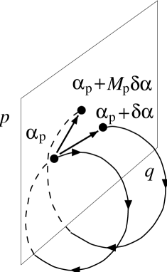
Fig. 1: Illustrates the nearby orbit problem for a classical map. Shown is a periodic orbit ${{\mbox{\boldmath$\alpha$}}}_{\rm p}$ and a nearby orbit starting at ${{\mbox{\boldmath$\alpha$}}}_{\rm p}+\delta{{\mbox{\boldmath$\alpha$}}}$ and leading to ${{\mbox{\boldmath$\alpha$}}}_{\rm p}+\tilde{M}_{\rm p}\delta{{\mbox{\boldmath$\alpha$}}}$ in time $t$.

(Here we consider ${\hat{\cal R}}(\tilde{M}_{t})$ in the extended domain.) We assume that the classical dynamics is hyperbolic. In this case, within the semiclassical approximation, the essential contributions to this trace will come from isolated, unstable periodic points ${{\mbox{\boldmath$\alpha$}}}_{\rm p}$ and we write (compare Fig. 1)

$${{\mbox{\boldmath$\alpha$}}}_{0}={{\mbox{\boldmath$\alpha$}}}_{\rm p}+\delta{{\mbox{\boldmath$\alpha$}}}\,,\qquad{{\mbox{\boldmath$\alpha$}}}_{t}={{\mbox{\boldmath$\alpha$}}}_{\rm p}+\tilde{M}_{\rm p}\,\delta{{\mbox{\boldmath$\alpha$}}}\,,$$ (49)

where $t=nT$, and $\tilde{M}_{\rm p}$ is the stability matrix evaluated at the periodic point. Using (22) and (24) one has for the matrix element in the vicinity of ${{\mbox{\boldmath$\alpha$}}}_{\rm p}$

$$\langle 0|\hat{\cal T}^{\dagger}({{\mbox{\boldmath$\alpha$}}}_{\rm p}+\delta{{\mbox{\boldmath$\alpha$}}})\,\hat{\cal T}({{\mbox{\boldmath$\alpha$}}}_{\rm p}+\tilde{M}_{\rm p}\delta{{\mbox{\boldmath$\alpha$}}})\,{\hat{\cal R}}(\tilde{M}_{\rm p}){|0\rangle}\sim\exp[{\rm i}{{\mbox{\boldmath$\alpha$}}}_{\rm p}\wedge(\tilde{M}_{\rm p}-\tilde{I})\delta{{\mbox{\boldmath$\alpha$}}}/2\hbar]$$ (50)

$$\hskip 199.16928pt\times\langle\delta{{\mbox{\boldmath$\alpha$}}}|{\hat{\cal R}}(\tilde{M}_{\rm p})|\delta{{\mbox{\boldmath$\alpha$}}}\rangle\,.$$

Consider the expansion of the phase in (48) about the phase value $R_{\rm p}$ characterising the period orbit. From (42), the difference $\delta\gamma_{t}$ between the phases characterising two nearby trajectories satisfies the following differential equation:

$$\delta\dot{\gamma}_{t}=-{\textstyle{1\over 2}}\delta{{\mbox{\boldmath$\alpha$}}}_{t}\wedge\dot{{\mbox{\boldmath$\alpha$}}}_{t}-{\textstyle{1\over 2}}{{\mbox{\boldmath$\alpha$}}}_{t}\wedge\delta\dot{{\mbox{\boldmath$\alpha$}}}_{t}-{\textstyle{1\over 2}}\delta{{\mbox{\boldmath$\alpha$}}}_{t}\wedge\delta\dot{{\mbox{\boldmath$\alpha$}}}_{t}-\delta H=-{\textstyle{1\over 2}}{{\rm d}\over{\rm d}t}\bigl{(}{{\mbox{\boldmath$\alpha$}}}_{t}\wedge\tilde{M}_{t}\delta{{\mbox{\boldmath$\alpha$}}}\bigr{)}\,.$$ (51)

This equation must be solved subject to the boundary condition that $\delta\gamma_{0}=0$. The solution is

$$\delta\gamma_{t}=-{\textstyle{1\over 2}}{{\mbox{\boldmath$\alpha$}}}_{t}\wedge\tilde{M}_{t}\delta{{\mbox{\boldmath$\alpha$}}}+{\textstyle{1\over 2}}{{\mbox{\boldmath$\alpha$}}}_{0}\wedge\delta{{\mbox{\boldmath$\alpha$}}}$$ (52)

For a periodic orbit, ${{\mbox{\boldmath$\alpha$}}}_{t}={{\mbox{\boldmath$\alpha$}}}_{0}={{\mbox{\boldmath$\alpha$}}}_{\rm p}$, so that in the neighbourhood of such an orbit (with $\tilde{M}_{\rm p}=\tilde{M}_{t}$)

$$\delta\gamma=-{\textstyle{1\over 2}}{{\mbox{\boldmath$\alpha$}}}_{\rm p}\wedge(\tilde{M}_{\rm p}-\tilde{I})\delta{{\mbox{\boldmath$\alpha$}}}\,.$$ (53)

Expanding the phase in (48) in the vicinity of ${{\mbox{\boldmath$\alpha$}}}_{\rm p}$, one now obtains

$$R_{t}-p_{t}q_{t}/2+p_{0}q_{0}/2=R_{\rm p}-\textstyle{1\over 2}[{{\mbox{\boldmath$\alpha$}}}_{\rm p}\wedge(\tilde{M}_{\rm p}-\tilde{I})\delta{{\mbox{\boldmath$\alpha$}}}]+O(\delta{{\mbox{\boldmath$\alpha$}}}^{3})\,.$$ (54)

Taking everything together (note that all terms linear in $\delta{{\mbox{\boldmath$\alpha$}}}$ in the phase cancel) we obtain for the contribution ${\rm Tr}[\hat{U}_{t}]_{\rm p}$ of a periodic point ${{\mbox{\boldmath$\alpha$}}}_{\rm p}$ to the trace of $\hat{U}_{t}$:

$${\rm Tr}[\hat{U}_{t}]_{\rm p}\sim\exp({\rm i}R_{\rm p}/\hbar)\,\mbox{Tr}\,[{\hat{\cal R}}(\tilde{M}_{\rm p})]\,.$$ (55)

It thus turns out that the stability property of the periodic orbit is encoded in the trace of ${\hat{\cal R}}(\tilde{M}_{\rm p})$. Using (32) we have

$${\rm Tr}[\hat{U}_{t}]_{\rm p}\sim\frac{\exp({\rm i}R_{\rm p}/\hbar+{\rm i}\pi\nu_{\rm p}/2)}{\sqrt{|{\rm det}(\tilde{M}_{\rm p}-\tilde{I})|}}\,.$$ (56)

This contribution is summed over all periodic points and one obtains

$$\mbox{Tr}\,[\hat{U}_{T}^{n}]\sim\sum_{\stackrel{{\scriptstyle\mbox{\small periodic points $p$}}}{{\mbox{\small of order $n$ }}}}\frac{n_{p}\,\exp({\rm i}R_{p}/\hbar+{\rm i}\pi\nu_{\rm p}/2)}{\sqrt{|\det(\tilde{M}_{p}-\tilde{I})|}}\,,$$ (57)

where $p$ is now an integer index labeling the periodic points. The sum is over all periodic points, including primitive points and their repetitions. In the latter case, $n_{p}=n/r_{p}$ where $r_{p}$ is the order of repetition. With this result one finds for the density (13) of eigenphases

$$d(\theta)\sim\frac{N}{2\pi\hbar}-\frac{1}{\pi\hbar}\mbox{Im}\sum_{p}\frac{n_{p}\,\exp[{\rm i}(R_{p}-n_{p}r_{p}\theta)/\hbar+{\rm i}\pi\nu_{p}/2]}{\sqrt{|\det(\tilde{M}_{p}-\tilde{I})|}}\,.$$ (58)

This is Gutzwiller’s trace formula for chaotic maps, discussed in reference [19]. The first term is often called Weyl contribution and describes the average density of states.

4.2 Gutzwiller’s trace formula for chaotic Hamiltonian flows

In this section we consider chaotic Hamiltonian flows with $d=2$ degrees of freedom and a time-independent Hamilton function $H({{\mbox{\boldmath$q$}}},{{\mbox{\boldmath$p$}}})$. As in the previous section, a semiclassical approximation for the trace of the quantum-mechanical time evolution operator $\hat{U}_{t}$ will be derived, in order to find a semiclassical expression for the density of states. The trace $\mbox{Tr}\,[\hat{U}_{t}]$ will again be evaluated using coherent states, using (2). There are two contributions: a smooth part (Weyl term) due to very short orbits (corresponding to the first term in (58)) and oscillatory contributions from periodic orbits.

We consider the smooth part first. For very short times,

$$\langle{{\mbox{\boldmath$\alpha$}}}|\hat{U}_{t}|{{\mbox{\boldmath$\alpha$}}}\rangle\simeq\langle{{\mbox{\boldmath$\alpha$}}}|\hat{\cal T}(\delta{{\mbox{\boldmath$\alpha$}}}_{t})|{{\mbox{\boldmath$\alpha$}}}\rangle\,{\rm e}^{\displaystyle-\frac{{\rm i}}{\hbar}H({{\mbox{\boldmath$\alpha$}}})t}$$ (59)

where $\delta{{\mbox{\boldmath$\alpha$}}}_{t}={{\mbox{\boldmath$\alpha$}}}_{t}-{{\mbox{\boldmath$\alpha$}}}$. If the coherent states are those of the Hamiltonian $H({{\mbox{\boldmath$\alpha$}}})={1\over 2}{{\mbox{\boldmath$\alpha$}}}.{{\mbox{\boldmath$\alpha$}}}$, then we may write

$$\langle{{\mbox{\boldmath$\alpha$}}}|\hat{\cal T}(\delta{{\mbox{\boldmath$\alpha$}}}_{t})|{{\mbox{\boldmath$\alpha$}}}\rangle\,=f(|\delta{{\mbox{\boldmath$\alpha$}}}_{t}|/\hbar)$$ (60)

where $|{{\mbox{\boldmath$\alpha$}}}|$ is the Euclidean norm of $\alpha$, (and the function $f(x)$ is a Gaussian, satisfying $f(0)=1$). Thus the smooth part of the density is

$$\langle\rho(E)\rangle \sim \int\!\frac{{\rm d}{{\mbox{\boldmath$\alpha$}}}}{(2\pi\hbar)^{2}}\,\int_{-\infty}^{\infty}\frac{{\rm d}t}{2\pi\hbar}\,{\rm e}^{\displaystyle{\rm i}[E-H({{\mbox{\boldmath$\alpha$}}})]t/\hbar}f(|\delta\dot{{\mbox{\boldmath$\alpha$}}}|t/\hbar)$$

$$= \int\frac{{\rm d}{{\mbox{\boldmath$\alpha$}}}}{(2\pi\hbar)^{2}}\,{1\over{|\dot{{\mbox{\boldmath$\alpha$}}}_{t}|\sqrt{\hbar}}}\widetilde{f}[(E-H({{\mbox{\boldmath$\alpha$}}})/|\delta\dot{{\mbox{\boldmath$\alpha$}}}_{t}|\sqrt{\hbar}]$$

where $\widetilde{f}(y)$ is the Fourier transform of $f(x)$. Now, noting that

$$\lim_{\epsilon\to 0}{1\over\epsilon}\tilde{f}(x/\epsilon)=f(0)\delta(x)\,,$$ (62)

the contribution to the density of states from short times is

$$\langle\rho(E)\rangle\sim\int\!\frac{{\rm d}{{\mbox{\boldmath$\alpha$}}}}{(2\pi\hbar)^{2}}\,\delta[E-H({{\mbox{\boldmath$\alpha$}}})]\,,$$ (63)

which is the well known Weyl estimate [3].

We now turn to the periodic-orbit contributions. The derivation of the previous section needs to be slightly modified since (as we shall shortly show) the stability matrix for a flow always has an eigenvalue unity (along the direction of the flow). Thus the representation (25) is singular. The solution to this problem is to treat longitudinal and transverse coordinates separately, as described in the following.

It will be helpful to introduce a local canonical coordinate system in the vicinity of an unstable periodic orbit. The reference orbit is denoted by ${{\mbox{\boldmath$\alpha$}}}_{\rm p}(\tau,\eta)$, with $\tau$ measuring the time taken a reach the point ${{\mbox{\boldmath$\alpha$}}}_{\rm p}(\tau,\eta)$ from some arbitrary starting point on the orbit at energy $\eta$. The period of the orbit is $T_{\rm p}(\eta)$. Any point close to the orbit may be specified by giving its deviation from some point on the reference orbit: ${{\mbox{\boldmath$\alpha$}}}={{\mbox{\boldmath$\alpha$}}}_{\rm p}(\tau,\eta)+\delta{{\mbox{\boldmath$\alpha$}}}$, where $\delta{{\mbox{\boldmath$\alpha$}}}$ depends upon $\tau$ and $\eta$. For points close to the orbit at a reference energy $\eta_{0}$, we will find it convenient to represent the deviations by a transformed set of local canonical coordinates, $\delta{{\mbox{\boldmath$\alpha$}}}^{\prime}$, such that

$$\delta{{\mbox{\boldmath$\alpha$}}}=\tilde{M}^{\prime}(\tau)\delta{{\mbox{\boldmath$\alpha$}}}^{\prime}\ ,\ \ \ \delta{{\mbox{\boldmath$\alpha$}}}^{\prime}=(\delta\tau,\delta E,\delta X,\delta P)\,,$$ (64)

where $\tilde{M}^{\prime}$ is a symplectic matrix depending upon $\tau$. This matrix is chosen so that the new coordinates $\delta{{\mbox{\boldmath$\alpha$}}}$ have the following interpretations. The energy $\delta E$ is defined by $\delta E=H({{\mbox{\boldmath$\alpha$}}})-\eta_{0}$. The time coordinate $\delta\tau$ measures the contribution to the displacement $\delta{{\mbox{\boldmath$\alpha$}}}$ from a vector parallel to the flow, namely $\tilde{J}\partial H/\partial{{\mbox{\boldmath$\alpha$}}}$. The remaining coordinates $\delta{{\mbox{\boldmath$\beta$}}}=(\delta X,\delta P)$ measure perpendicular displacements from the orbit; they are chosen such that $\delta{{\mbox{\boldmath$\beta$}}}=0$ corresponds to a point on the reference periodic orbit at energy $\eta_{0}+\delta E$. The construction of the symplectic transformation $\tilde{M}^{\prime}(\tau)$ is described in an appendix. Note that this symplectic transformation is periodic: $\tilde{M}^{\prime}(\tau+T_{\rm p}(\eta_{0}))=\tilde{M}^{\prime}(\tau)$.

Given an initial deviation $\delta{{\mbox{\boldmath$\alpha$}}}$ from the reference trajectory ${{\mbox{\boldmath$\alpha$}}}_{\rm p}(\tau,\eta_{0})$ at time $t=0$, there will be a corresponding deviation ${{\mbox{\boldmath$\alpha$}}}_{t}$ from ${{\mbox{\boldmath$\alpha$}}}_{\rm p}(\tau+t,\eta_{0})$ at a later time $t$. We write

$$\delta{{\mbox{\boldmath$\alpha$}}}_{t}=\tilde{M}^{\prime}(t+\tau)\delta{{\mbox{\boldmath$\alpha$}}}^{\prime}_{t}\ ,\ \ \ \delta{{\mbox{\boldmath$\alpha$}}}^{\prime}_{t}=\tilde{M}^{\prime\prime}_{t}\delta{{\mbox{\boldmath$\alpha$}}}^{\prime}\,,$$ (65)

where $\tilde{M}^{\prime\prime}_{t}$ is a monodromy matrix which describes the instability of the orbit in the local canonical coordinates $\delta{{\mbox{\boldmath$\alpha$}}}^{\prime}$. The construction of the $\delta{{\mbox{\boldmath$\alpha$}}}^{\prime}$ coordinates implies that there is no coupling between the deviation in the $(\delta E,\delta\tau)$ subspace and the delta $\delta{{\mbox{\boldmath$\beta$}}}$ subspace.

$$\delta{{\mbox{\boldmath$\alpha$}}}^{\prime}=\bigl{(}\delta\tau,\delta\eta,\delta{{\mbox{\boldmath$\beta$}}}\bigr{)}\,,\qquad\delta{{\mbox{\boldmath$\alpha$}}}^{\prime}_{t}=\bigl{(}\delta\tau+\frac{\partial t}{\partial E}\delta\eta,\delta\eta,\tilde{M}_{\perp}\delta{{\mbox{\boldmath$\beta$}}}\bigr{)}\,,$$ (66)

so that the stability matrix $\tilde{M}^{\prime\prime}_{t}$ has the following form

$$\tilde{M}^{\prime\prime}_{t}=\left(\begin{array}[]{cc}\tilde{M}_{||}&\tilde{0}\\ \tilde{0}&\tilde{M}_{\perp}\end{array}\right)$$ (67)

where $\tilde{M}$ and $\tilde{M}_{\perp}$ are $2\times 2$ symplectic matrices, with

$$\tilde{M}_{||}=\left(\begin{array}[]{cc}1&b\\ 0&1\end{array}\right)\,,$$ (68)

and $b={\rm d}t/{\rm d}E$, and $\tilde{M}_{\perp}$ is a $2(d-1)\times 2(d-1)$ symplectic matrix mapping infinitesimal deviations in the transverse coordinates. In the fixed canonical coordinate system, the stability matrix describing the evolution of small deviations $\delta{{\mbox{\boldmath$\alpha$}}}$ from the reference trajectory is $\tilde{M}_{t}=\tilde{M}^{\prime}(t+\tau)\tilde{M}^{\prime\prime}_{t}[\tilde{M}^{\prime}(\tau)]^{-1}$.

Evaluation of the trace ${\rm Tr}[\hat{U}_{t}]$ follows the approach used in section 4.1, and requires the evaluation of $\langle\delta{{\mbox{\boldmath$\alpha$}}}|{\hat{\cal R}}(\tilde{M}_{t})|\delta{{\mbox{\boldmath$\alpha$}}}\rangle$. The metaplectic operator ${\hat{\cal R}}(\tilde{M}_{t})$ must be considered a a continuous function of $t$, defined in the extended domain. It may be written as a product, so that when $t\approx T_{\rm p}(\eta_{0})$:

$${\rm Tr}\bigl{[}{\hat{\cal R}}(\tilde{M}_{t})\bigr{]} = {\rm Tr}\bigl{[}{\hat{\cal R}}(\tilde{M}^{\prime}(t+\tau)){\hat{\cal R}}(\tilde{M}^{\prime\prime}_{t})[{\hat{\cal R}}(\tilde{M}^{\prime}(\tau))]^{-1}\bigr{]}$$ (69)

$$= (-1)^{s}{\rm Tr}\bigl{[}{\hat{\cal R}}(\tilde{M}^{\prime}(\tau)){\hat{\cal R}}(\tilde{M}_{t}^{\prime\prime})[{\hat{\cal R}}(\tilde{M}(\tau))]^{-1}\biggr{]}$$

$$= (-1)^{s}{\rm Tr}\bigl{[}{\hat{\cal R}}(\tilde{M}^{\prime\prime}_{t})\bigr{]}\,.$$

Here we have used the fact that $\tilde{M}^{\prime}(\tau)$ is periodic, so that ${\hat{\cal R}}(\tilde{M}^{\prime}(\tau))$ is periodic apart from a factor $(-1)^{s}$ discussed in section 3.3.

The operator ${\hat{\cal R}}(\tilde{M}^{\prime\prime}_{t})$ may be written in the form

$${\hat{\cal R}}(\tilde{M}^{\prime\prime}_{t})=\left(\begin{array}[]{cc}{\hat{\cal R}}(\tilde{M}_{\perp})&\hat{0}\\ \hat{0}&{\hat{\cal R}}(\tilde{M})\end{array}\right)$$ (70)

where ${\hat{\cal R}}(M)$ and ${\hat{\cal R}}(M_{\perp})$ are operators acting upon Hilbert spaces corresponding to respectively one and $d-1$ degrees of freedom. These operators may be expressed as integrals of the form (25), constructed using sets of mutually commuting translation operators, respectively $\hat{\cal T}(\tau,\eta)$ and $\hat{\cal T}({{\mbox{\boldmath$\beta$}}})$. This implies that the matrix element of the metaplectic operator ${\hat{\cal R}}(\tilde{M}^{\prime\prime}_{t})$ is in the form of a product

$$\langle\delta{{\mbox{\boldmath$\alpha$}}}|{\hat{\cal R}}(\tilde{M}^{\prime\prime}_{t})|\delta{{\mbox{\boldmath$\alpha$}}}\rangle=\langle\delta\tau,\delta\eta|{\hat{\cal R}}(\tilde{M}_{||})|\delta\tau,\delta\eta\rangle\,\langle\delta{{\mbox{\boldmath$\beta$}}}|{\hat{\cal R}}(\tilde{M}_{\perp})|\delta{{\mbox{\boldmath$\beta$}}}\rangle\,.$$ (71)

We now evaluate a contribution to ${\rm Tr}[\hat{U}_{t}]$ arising from a periodic orbit. The dominant contribution arises for period orbits of period $T_{\rm p}=t$, and we choose the energy $\eta$ such that this condition is satisfied. Following the argument leading from (48) to (55), the contribution to the trace is

$$\mbox{Tr}[\hat{U}_{t}]_{\rm p} = {(-1)^{s}\over{(2\pi\hbar)^{2}}}\int_{0}^{T_{\rm p}}{\rm d}\tau\int_{-\infty}^{\infty}{\rm d}\delta\eta\int{\rm d}\delta{{\mbox{\boldmath$\beta$}}}\ \langle{{\mbox{\boldmath$\alpha$}}}_{\rm p}+\delta{{\mbox{\boldmath$\alpha$}}}|\hat{U}_{t}|{{\mbox{\boldmath$\alpha$}}}_{\rm p}+\delta{{\mbox{\boldmath$\alpha$}}}\rangle$$ (72)

$$= {\exp({\rm i}R_{\rm p}/\hbar+{\rm i}\pi s)\over{2\pi\hbar}}\int_{0}^{T_{\rm p}}\!\!{\rm d}\tau\,\int_{-\infty}^{\infty}\!\!{\rm d}\delta\eta\ \langle\delta\eta\ |{\hat{\cal R}}(\tilde{M}_{||})|\delta\eta\rangle\ \mbox{Tr}\,[{\hat{\cal R}}(\tilde{M}_{\perp})]$$

where $R_{\rm p}$ is the action of the periodic orbit, with the energy $\eta$ chosen such that $T_{\rm p}(\eta)=t$. Using Eqs. (32) and (34), and performing the integral over $\tau$, this evaluates to

$$\mbox{Tr}[\hat{U}_{t}]_{\rm p}={T_{\rm p}\over{\sqrt{2\pi{\rm i}\hbar b_{\rm p}}}}{\exp[{\rm i}R_{\rm p}/\hbar+{\rm i}\pi(\mu_{\rm p}+2s)/2)]\over{\sqrt{|\det(\tilde{M}_{\perp}-\tilde{I})|_{\rm p}}}}\,.$$ (73)

where $\tilde{M}_{\perp}$ is evaluated for the periodic orbit with period $T_{\rm p}=t$, and $\mu_{\rm p}$ is an additional index chosen so that ${\hat{\cal R}}(\tilde{M}_{\perp})$ is a continuous function of time along the periodic orbit. This expression is an explicit function of $\eta$, but implicitly a function of $t$, since $\eta$ satisfies $t=T_{\rm p}(\eta)$.

Now the time integral over $\mbox{Tr}[\hat{U}_{t}]$ is performed, in order to evaluate the density of states. The contribution due to a single family of periodic orbits is

$$\rho(E)=\int_{-\infty}^{\infty}\frac{{\rm d}t}{2\pi\hbar}\ \exp({\rm i}Et/\hbar)\,{\rm Tr}[\hat{U}_{t}]_{\rm p}\,.$$ (74)

This integral is approximated using the method of stationary phase. The time is written $t=t_{0}+\delta t$ where $t_{0}$, the stationary phase point, satisfies

$${\frac{{\rm d}}{{\rm d}t}}(Et+R_{\rm p})=0\qquad\mbox{for $t=t_{0}$}\,.$$ (75)

We will discuss the solution of this equation in detail. For each value of the time $t$ over which we integrate, the integrand is evaluated at a different value of the energy, $\eta$, determined by the implicit relation $t=T_{\rm p}(\eta)$. The action $S_{\rm p}$ of the orbit and its period $T_{\rm p}$ are also functions of the energy $\eta$:

$$S_{\rm p}(\eta)=\oint{{{\mbox{\boldmath$p$}}}}.{\rm d}{{{\mbox{\boldmath$q$}}}}\bigg{|}_{({{{\mbox{\boldmath$q$}}}},{{{\mbox{\boldmath$p$}}}})={{\mbox{\boldmath$\alpha$}}}_{\rm p}(\tau)}\ ,\ \ \ \ T_{\rm p}={\partial S_{\rm p}\over{\partial\eta}}\,.$$ (76)

The equation (75) for the stationary phase condition now becomes

$$0 = {{\rm d}\over{{\rm d}t}}\big{\{}S_{\rm p}[\eta(t)]-\eta(t)t+Et\big{\}}=[T_{\rm p}(\eta)-t]{{\rm d}\eta\over{{\rm d}t}}+[E-\eta(t)]\,.$$ (77)

We have already required that $T_{\rm p}(\eta)=t$ and we therefore satisfy the stationary phase condition by requiring, in addition, that $E=\eta(t)$. When evaluating the integral (74), the value of the energy $E$ therefore determines $\eta=E$, which in turn determines the stationary phase point $t_{0}=T_{\rm p}(\eta)$. We note that this corresponds to a Legendre transformation from $R$ to $S$:

$$S_{\rm p}=R_{\rm p}+Et\,,\qquad\frac{\partial R_{\rm p}}{\partial t}=-E\,.$$ (78)

In order to perform the stationary phase integral, we require the second derivative of the action: we write

$$Et+S_{\rm p}(\eta(t))-\eta t=S_{\rm p}(E)+{\textstyle{1\over 2}}\lambda[t-T_{\rm p}(E)]^{2}$$ (79)

where we find

$$\lambda=-{{\rm d}E\over{{\rm d}T_{\rm p}}}=-b^{-1}|_{\rm p}\,.$$ (80)

The Gaussian integration over $\delta t$ gives a factor of $\exp({\rm i}\pi/2)\sqrt{2\pi{\rm i}\hbar b_{\rm p}}$, and thus we obtain for the contribution of a periodic orbit to the density of states

$$\frac{1}{2\pi\hbar}\frac{T_{\rm p}\,\exp\bigl{(}{\rm i}S_{\rm p}/\hbar+{\rm i}\pi\nu_{\rm p}/2\bigr{)}}{\sqrt{|\det(\tilde{M}_{\perp}-\tilde{I})|_{\rm p}}}$$ (81)

where $\nu_{\rm p}=\mu_{\rm p}+2s+1$ is the Maslov index of the periodic orbit. By summing over individual contributions from isolated, hyperbolic periodic orbits, labeled by an index $p$. Combining contributions from positive- and negative-time orbits one obtains:

$$\rho(E)=\langle\rho(E)\rangle+\frac{1}{\pi\hbar}\mbox{Re}\sum_{p}{{T_{p}}\over{\sqrt{|{\rm det}(\tilde{M}_{\perp}-\tilde{I})|_{p}}}}\exp\biggl{(}{{\rm i}S_{p}\over{\hbar}}+{{\rm i}\pi\nu_{p}\over 2}\biggr{)}\,.$$ (82)

This is Gutzwiller's trace formula [1, 2, 3].

4.3 More general trace formulae for chaotic Hamiltonian flows

The results of the previous section may be used to derive semiclassical approximations for more general traces, such as $\mbox{Tr}\,[\hat{A}\,\hat{U}_{t}]$, where $\hat{A}$ is an observable with a classical limit $A({{\mbox{\boldmath$\alpha$}}})$, compare Eq. (9). This trace may be written as

$$\mbox{Tr}\,\bigl{[}\hat{A}\hat{U}_{t}\bigr{]}=\int\!\frac{{\rm d}{{\mbox{\boldmath$\alpha$}}}}{(2\pi\hbar)^{d}}\ A({{\mbox{\boldmath$\alpha$}}})\ \langle{{\mbox{\boldmath$\alpha$}}}|\hat{U}_{t}|{{\mbox{\boldmath$\alpha$}}}\rangle\,.$$ (83)

Using (59) one obtains for the smooth part of the density $\rho_{A}(E)$ [20]

$$\langle\rho_{A}(E)\rangle=\int\!\frac{{\rm d}{{\mbox{\boldmath$\alpha$}}}}{(2\pi\hbar)^{d}}\,A({{\mbox{\boldmath$\alpha$}}})\,\delta[E-H({{\mbox{\boldmath$\alpha$}}})]\,.$$ (84)

As far as the periodic-orbit contributions are concerned, it is immediately obvious that all steps performed in section 4.2 are the same in this case, except for an additional factor of $A(\tau,E)$ . One thus obtains for the weighted density [12]

$$\rho_{A}(E)=\langle\rho_{A}(E)\rangle+\frac{1}{\pi\hbar}\mbox{Re}\sum_{p}\frac{A_{p}}{\sqrt{|\det({\tilde{M}_{\perp}}-\tilde{I})|_{p}}}\,\exp\biggl{(}{{\rm i}S_{p}\over\hbar}+{{\rm i}\pi\nu_{p}\over 2}\biggr{)}\,.$$ (85)

where $A_{p}$ is the average of the observable $A({{\mbox{\boldmath$\alpha$}}})$ over the $p^{\rm th}$ orbit:

$$A_{p}=\int_{0}^{T_{p}}\!{\rm d}t\ A({{\mbox{\boldmath$\alpha$}}}_{t})\,.$$ (86)

Similarly, a trace formula involving non-diagonal matrix elements may be derived, starting from the expression

$$S_{A}(t,s)=\mbox{Tr}[\hat{A}\,\hat{U}_{s}\,\hat{A}\,\hat{U}_{t-s}]\,.$$ (87)

We may write

$$S_{A}(t,s)={1\over{(2\pi\hbar)^{d}}}\int\!\frac{{\rm d}{{\mbox{\boldmath$\alpha$}}}}{(2\pi\hbar)^{2}}\,A({{\mbox{\boldmath$\alpha$}}})\,A({{\mbox{\boldmath$\alpha$}}}_{s})\,\langle{{\mbox{\boldmath$\alpha$}}}|\hat{U}_{t}|{{\mbox{\boldmath$\alpha$}}}\rangle\,.$$ (88)

Using (59), one has [20, 7]

$$\langle S_{A}(E,\hbar\omega)\rangle=\int_{-\infty}^{\infty}\!\frac{{\rm d}s}{2\pi\hbar}\,{\rm e}^{\displaystyle i\omega s}\int\!\frac{{\rm d}{{\mbox{\boldmath$\alpha$}}}}{(2\pi\hbar)^{d}}\,A({{\mbox{\boldmath$\alpha$}}})\,A({{\mbox{\boldmath$\alpha$}}}_{s})\,\delta[E-H({{\mbox{\boldmath$\alpha$}}})]\,,$$ (89)

which is just the Fourier transform of the phase-space averaged correlation function, as derived in [7]. Including the periodic-orbit contributions one obtains the following expression

$$S_{A}(E,\hbar\omega)=\langle S_{A}(E,\hbar\omega)\rangle+\frac{1}{\pi\hbar}\mbox{Re}\sum_{p}\frac{S_{p}(E,\hbar\omega)}{\sqrt{|\det({\tilde{M}_{\perp}}-\tilde{I})|_{p}}}\,\exp\biggl{(}{{\rm i}S_{p}\over{\hbar}}+{{\rm i}\pi\nu_{p}\over 2}\biggr{)}$$ (90)

where

$$S_{p}(E,\hbar\omega)=\int_{-\infty}^{\infty}\!\frac{{\rm d}s}{2\pi\hbar}\,{\rm e}^{\displaystyle{\rm i}\omega s}\int_{0}^{T_{p}}\!{\rm d}t\,A({{\mbox{\boldmath$q$}}}_{t+s},{{\mbox{\boldmath$p$}}}_{t+s})\,A({{\mbox{\boldmath$\alpha$}}}_{t},{{\mbox{\boldmath$p$}}}_{t})\,.$$ (91)

5 Discussion

We close with a couple of additional remarks. First, the above formulae were derived assuming that all periodic orbits are isolated and unstable (as is the case in hyperbolic systems). The above approach is very easily extended to deal with integrable systems where the dynamics is most conveniently expressed in angle and action variables ${{\mbox{\boldmath$\alpha$}}}=({{\mbox{\boldmath$\theta$}}},{{\mbox{\boldmath$I$}}})$. In these variables, the Hamilton function is a function of the action variables only, $H({{\mbox{\boldmath$I$}}})$. Thus

$${{\mbox{\boldmath$I$}}}_{t}={\rm const.}\,,\qquad{{\mbox{\boldmath$\theta$}}}_{t}={{\mbox{\boldmath$\theta$}}}+{{\mbox{\boldmath$\omega$}}}({{\mbox{\boldmath$I$}}})\,t$$ (92)

with ${{\mbox{\boldmath$\omega$}}}({{\mbox{\boldmath$I$}}})=\partial H/\partial{{\mbox{\boldmath$I$}}}$. The for the typical case where the frequencies are not rationally related, the trajectories fill $d$ dimensional tori in phase space. The periodic orbits only occur when the frequencies are rationally related, which occurs when the actions ${{\mbox{\boldmath$I$}}}({{\mbox{\boldmath$\nu$}}})$ satisfy the implicit equation

$${{\mbox{\boldmath$\omega$}}}[{{\mbox{\boldmath$I$}}}({{\mbox{\boldmath$\nu$}}})]t=2\pi{{\mbox{\boldmath$\nu$}}}\,.$$ (93)

where ${{\mbox{\boldmath$\nu$}}}=(\nu_{1},\nu_{2},\ldots)$ is a vector of integers. The trajectories labeled by the integer vectors $\nu$ form $d$-parameter families (rational tori) which can be labeled by an initial angle ${{\mbox{\boldmath$\theta$}}}_{0}$. It is thus clear that the leading-order contribution to the trace (2) comes from periodic orbits on rational tori. The derivation of the trace formula for integrable systems [11] proceeds exactly as before, using a $2d$-dimensional generalization of the representation (34).

Secondly, it is clear that the trace formulae Eqs. (8), (82), (85) and (90) are not exact and at best asymptotically valid for small $\hbar$. In order to obtain convergent expressions, the densities (4-6) are often smoothed by convolution with a smoothing factor, i.e.,

$$\rho_{\epsilon}(E)=\frac{1}{\sqrt{2\pi}\epsilon}\,\int_{-\infty}^{\infty}\!{\rm d}E^{\prime}\,\rho(E^{\prime})\,\exp[-(E-E^{\prime})^{2}/2\epsilon^{2}]\,.$$ (94)

This leads to a truncation of the periodic orbit sums in (82), (85) and (90) [7]. The periodic-orbit formulae (82) and (85) are certainly valid provided the wave packet does not spread to the extent that the use of a linearised approximation to describe its deformation becomes invalid. If the system is hyperbolic, this criterion leads to the requirement that $\epsilon>\hbar\lambda/\mbox{log}(S_{0}/\hbar)$, where $\lambda$ is an exponent describing the exponential separation of trajectories, and $S_{0}$ a characteristic action scale for the system. In the case of (89), an additional smoothing with respect to the second argument of $S_{A}$ is needed, of the same order of magnitude as $\epsilon$.

Appendix
This appendix explains the construction of the coordinate system used in section 4.2. It is constructed around a periodic orbit. The set of points on the periodic orbit is ${{\mbox{\boldmath$\alpha$}}}_{\rm p}(\tau,\eta)$, where $\eta$ is the energy and $\tau$ is the time taken to reach the point starting from an arbitrary reference point. We assume that these reference points are chosen such that ${{\mbox{\boldmath$\alpha$}}}(\tau,\eta)$ is a smooth function of $\tau$.

Local canonical coordinates $(\delta\tau,\delta\eta,\delta X,\delta P)=(\delta\alpha^{\prime}_{1},\delta\alpha^{\prime}_{2},\delta\alpha^{\prime}_{3},\delta\alpha^{\prime}_{4})=\delta{{\mbox{\boldmath$\alpha$}}}^{\prime}$ are constructed from the original coordinates $(x,y,p_{x},p_{y})$ by obtaining a set of four vectors ${\bf v}_{i}$, such that $\sum_{i}{\bf v}_{i}\delta\alpha^{\prime}_{i}$ is the variation of $(x,y,p_{x},p_{y})$ resulting from a variation of the new coordinates. The vector ${\bf v}_{1}$ is the velocity vector of the Hamiltonian flow, ${\bf v}_{1}=\tilde{J}(\partial H/\partial{{{\mbox{\boldmath$\alpha$}}}})$. The vector ${\bf v}_{2}=\partial{{\mbox{\boldmath$\alpha$}}}_{\rm p}(\tau,\eta)/\partial\eta$ satisfies ${\bf v}_{1}^{\rm T}\tilde{J}{\bf v}_{2}=1$, so that the coordinates $\delta\alpha_{1}^{\prime}=\delta\tau$ and $\delta\alpha_{2}^{\prime}=\delta\eta$ form a canonical pair. The remaining vectors ${\bf v}_{3}$ and ${\bf v}_{4}$ are constructed so that $\gamma_{ij}={\bf v}_{i}^{\rm T}\tilde{J}{\bf v}_{j}$ satisfies $\gamma_{ij}=0$ when $i\in\{1,2\}$ and $j\in\{3,4\}$, and $\gamma_{34}=1$. These values of $\gamma_{ij}$ represent five linear constraints on the eight coefficients defining the vectors ${\bf v}_{3}$ and ${\bf v}_{4}$. All of these vectors are functions of $\tau$. The matrix element $M_{ij}^{\prime}(\tau)$ of $\tilde{M}^{\prime}(\tau)$ is the $i^{\rm th}$ component of the vector ${\bf v}_{j}$.

References

- [1] M. C. Gutzwiller, J. Math. Phys. 8 (1967) 1979
- [2] M. C. Gutzwiller, J. Math. Phys. 12 (1971) 343
- [3] M. C. Gutzwiller, Chaos in Classical and Quantum Mechanics, Springer: New York (1990)
- [4] N. Balazs and A. Voros, Phys. Rep. 143 (1987) 109
- [5] H. Friedrich and D. Wintgen, Phys. Rep. 183 (1989) 37
- [6] G. Montambaux, in: Quantum Fluctuations, Les Houches proceedings 1995, eds: E. Giacobino, S. Reynaud and J. Zinn-Justin, Elsevier (1998)
- [7] M. Wilkinson, J. Phys. A: Math. Gen. 20 (1987) 2415
- [8] M. Combescure, D. Robert, and J. Ralston, Commun. Math. Phys. 202 (1999) 463
- [9] R. G. Littlejohn, Phys. Rep. 138 (1986) 193
- [10] M. Wilkinson, J. Phys.: Condensed Matter 10 (1998) 7407
- [11] M. Berry and M. V. Tabor, J. Phys. A: Math. Gen. 10 (1977) 371
- [12] M. Wilkinson, J. Phys. A: Math. Gen. 21 (1988) 1173
- [13] E. Merzbacher, Quantum Mechanics, 2nd ed., Wiley, New York (1970)
- [14] V. Bargmann, Comm. Pure Appl. Math. 14 (1961) 187
- [15] H. J. Groenewold, Physica 12 (1946) 405
- [16] S. R. de Groot and L. G. Suttorp, Foundations of Electrodynamics, North-Holland: Amsterdam (1972)
- [17] G. B. Folland, Harmonic Analysis in Phase Space, Princeton University Press: Princeton (1989)
- [18] V. P. Maslov and M. V. Fedoriuk, Semiclassical approximations in quantum mechanics, Reidel: Boston (1981)
- [19] U. Smilansky, in: Quantum Fluctuations, Les Houches proceedings 1995, eds: E. Giacobino, S. Reynaud and J. Zinn-Justin, Elsevier (1998)
- [20] M. Feingold and A. Peres, Phys. Rev. A 31 (1985) 2472