Universal eigenvector statistics in a quantum scattering ensemble

Abstract

We calculate eigenvector statistics in an ensemble of non-Hermitian matrices describing open quantum systems [F. Haake et al., Z. Phys. B 88, 359 (1992)] in the limit of large matrix size. We show that ensemble-averaged eigenvector correlations corresponding to eigenvalues in the center of the support of the density of states in the complex plane are described by an expression recently derived for Ginibre’s ensemble of random non-Hermitian matrices.

The statistical properties of eigenvector overlaps may have an important bearing on time evolution and determine the sensitivity to perturbations of systems governed by non-Hermitian operators or matrices. In such systems it is thus important to know the statistical properties of the (left and right) eigenvectors. Despite this fact little is known about eigenvector correlations in general ensembles of non-Hermitian random matrices. In Refs. [1, 2], eigenvector statistics were calculated for Ginibre’s ensemble of random non-Hermitian matrices where each matrix element is an independent, identically distributed Gaussian complex random variable. The question arises to which extent these results are relevant for other ensembles of non-Hermitian random matrices.

In the following we determine eigenvector statistics for an ensemble of non-Hermitian $N\times N$ matrices of the form

$$J=H+{\rm i}\gamma\sum_{a=1}^{M}V^{a}({{V}^{a})}^{\dagger}\,.$$ (1)

Here $H$ is a $N\times N$ Hermitian random matrix with complex, Gaussian distributed matrix elements $H_{kl}$ with zero mean and variance $\langle|H_{kl}|^{2}\rangle=\delta_{kl}\,N^{-1}$ . The $V^{a}$ are vectors with complex random Gaussian entries $V_{k}^{a}$ with zero mean and variance $\langle V_{k}^{a}\overline{V}_{l}^{b}\rangle=\delta_{kl}\delta_{ab}N^{-1}$. The eigenvalues, $\lambda_{\alpha}$, of $J$ are distributed in the complex plane. The ensemble (1), with $\gamma<0$, has been used to model the statistical properties of resonances arising in the case of resonance scattering in open quantum systems [4, 5]; the position of the resonances is modelled by the real part $\lambda_{\alpha}^{\prime}$ of the eigenvalues of (1) and the width by the imaginary part $\lambda_{\alpha}^{\prime\prime}$. The statistics of eigenvectors for such an ensemble was found to be of considerable importance for describing the properties of random lasing media, see [6].

The ensemble-averaged density of states $d(z)=\big{\langle}N^{-1}\sum_{\alpha}\delta(z-\lambda_{\alpha})\big{\rangle}$ for the ensemble (1) has been worked out using a number of different techniques, namely the replica trick [3], the non-linear sigma model approach [5] and using the self-consistent Born approximation [7].

Very recently, in Ref. [8], all $n$-point spectral correlation functions for a variant of the ensemble (1) were determined. It is given by

$$J=H+{\rm i}\Gamma$$ (2)

where $H$ is defined as above, and $\Gamma$ is a fixed, $N\times N$ diagonal matrix with $M$ non-zero diagonal matrix elements $\gamma$. For the ensemble (2) it was shown, in particular, that the spectral two-point function $R_{2}(z_{1},z_{2})=\big{\langle}N^{-1}\sum_{\alpha\neq\beta}\delta(z_{1}-\lambda_{\alpha})\delta(z_{2}-\lambda_{\beta})\big{\rangle}$ (and all higher correlation functions) are – after suitable rescaling and sufficiently far away from the boundary of the support of the spectrum – identical to those derived for Ginibre’s ensemble (see Eqs. (15.1.31) and (15.1.37) of Ref. [10]). One thus expects that spectral $n$-point correlations of the ensemble (1) are locally similar to those in Ginibre’s ensemble and thus universal. Furthermore it has been argued that under very general circumstances the fluctuations of the ensembles (1) and (2) are identical [9].

Below, we explore to which extent the statistical properties of eigenvectors in the ensembles (1) and (2) are universal and the remainder of this paper is organized as follows. After defining the eigenvector correlator to be calculated, we briefly discuss the method used: the self-consistent Born approximation. We then derive an expression for eigenvector correlations and compare it to results of previous calculations for Ginibre’s ensemble [1, 2]. Finally, we show results of numerical simulations, compare them to our analytical results, and discuss the applicability of our analytical method.

The eigenvalues of (1) are non-degenerate with probability one, and in this case the left and right eigenvectors, $|L_{\alpha}\rangle$ and $|R_{\alpha}\rangle$,

$$J\,|R_{\alpha}\rangle = \lambda_{\alpha}\,|R_{\alpha}\rangle\,,$$ (3)

$$\langle L_{\alpha}|\,J = \langle L_{\alpha}|\,\lambda_{\alpha}$$ (4)

form two complete, biorthogonal sets, and can be normalised so that

$$\langle L_{\alpha}|R_{\beta}\rangle=\delta_{\alpha\beta}\,.$$ (5)

We indicate Hermitian conjugates of vectors in the usual way, so that, for example, $|L_{\alpha}\rangle$ satisfies $J^{\dagger}\,|L_{\alpha}\rangle=\overline{\lambda}_{\alpha}\,|L_{\alpha}\rangle$. We investigate the eigenvector correlators [1, 2]

$$O(z) = \Big{\langle}\frac{1}{N}\sum_{\alpha}O_{\alpha\alpha}\,\delta(z-\lambda_{\alpha})\Big{\rangle}\,,$$ (6)

$$O(z_{1},z_{2}) = \Big{\langle}\frac{1}{N}\sum_{\alpha\neq\beta}O_{\alpha\beta}\,\delta(z_{1}-\lambda_{\alpha})\,\delta(z_{2}-\lambda_{\beta})\Big{\rangle}$$ (7)

where $O_{\alpha\beta}=\langle L_{\alpha}|L_{\beta}\rangle\,\langle R_{\beta}|R_{\alpha}\rangle$ . These quantities may be extracted from

$$D(z_{1},z_{2})=\Big{\langle}\frac{1}{N}\sum_{\alpha,\beta}O_{\alpha\beta}\,\delta(z_{1}-\lambda_{\alpha})\,\delta(z_{2}-\lambda_{\beta})\Big{\rangle}$$ (8)

which may be written as $D(z_{1},z_{2})=O(z_{1})\,\delta(z_{1}-z_{2})+O(z_{1},z_{2})$. An expression for the diagonal part $O(z_{1})$ for the ensemble (1) was derived in [11].

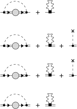
FIG. 1.: Shows a diagrammatic representation of the self-energy $\textstyle\Sigma$. For the diagrammatic rules see [2] and Fig. 2 below.

Self-consistent Born approximation. We calculate eigenvector correlators in terms of averages of products of Green functions, using an approximation scheme, namely an expansion in powers of $N^{-1}$. The method used in Refs. [1, 2], yielding exact results for Ginibre’s ensemble, is not readily generalizable. We use the approach developed in [7, 12, 13]: since the Green functions are non-analytic in the lower (upper) complex half-plane, a Hermitian $2N\times 2N$ matrix $\mathchoice{{\hbox{\boldmath$\displaystyle H$}}}{{\hbox{\boldmath$\textstyle H$}}}{{\hbox{\boldmath$\scriptstyle H$}}}{{\hbox{\boldmath$\scriptscriptstyle H$}}}=\mathchoice{{\hbox{\boldmath$\displaystyle H$}}}{{\hbox{\boldmath$\textstyle H$}}}{{\hbox{\boldmath$\scriptstyle H$}}}{{\hbox{\boldmath$\scriptscriptstyle H$}}}_{0}+\mathchoice{{\hbox{\boldmath$\displaystyle H$}}}{{\hbox{\boldmath$\textstyle H$}}}{{\hbox{\boldmath$\scriptstyle H$}}}{{\hbox{\boldmath$\scriptscriptstyle H$}}}_{1}$ is introduced [7, 12]

$$\mathchoice{{\hbox{\boldmath$\displaystyle H$}}}{{\hbox{\boldmath$\textstyle H$}}}{{\hbox{\boldmath$\scriptstyle H$}}}{{\hbox{\boldmath$\scriptscriptstyle H$}}}_{0}=\left(\begin{array}[]{cc}\eta&\\ &-\eta\end{array}\right)\,,\hskip 14.22636pt\mathchoice{{\hbox{\boldmath$\displaystyle H$}}}{{\hbox{\boldmath$\textstyle H$}}}{{\hbox{\boldmath$\scriptstyle H$}}}{{\hbox{\boldmath$\scriptscriptstyle H$}}}_{1}=\left(\begin{array}[]{cc}&A\\ A^{\dagger}&\end{array}\right)$$ (9)

with $\eta>0$, $A=z-J$ and with inverse

$$\mathchoice{{\hbox{\boldmath$\displaystyle G$}}}{{\hbox{\boldmath$\textstyle G$}}}{{\hbox{\boldmath$\scriptstyle G$}}}{{\hbox{\boldmath$\scriptscriptstyle G$}}}=\left(\begin{array}[]{cc}G_{11}&G_{12}\\ G_{21}&G_{22}\end{array}\right)\,.$$ (10)

The resolvents are obtained by taking $\eta\rightarrow 0$. In this limit, $G_{21}=(z-J)^{-1}$ and $G_{12}=(\overline{z}-J^{\dagger})^{-1}$. Expanding the Green function $\textstyle G$ as a power series in $\mathchoice{{\hbox{\boldmath$\displaystyle H$}}}{{\hbox{\boldmath$\textstyle H$}}}{{\hbox{\boldmath$\scriptstyle H$}}}{{\hbox{\boldmath$\scriptscriptstyle H$}}}_{1}$, its ensemble average $\langle\mathchoice{{\hbox{\boldmath$\displaystyle G$}}}{{\hbox{\boldmath$\textstyle G$}}}{{\hbox{\boldmath$\scriptstyle G$}}}{{\hbox{\boldmath$\scriptscriptstyle G$}}}\rangle$ can be written as

$$\langle\mathchoice{{\hbox{\boldmath$\displaystyle G$}}}{{\hbox{\boldmath$\textstyle G$}}}{{\hbox{\boldmath$\scriptstyle G$}}}{{\hbox{\boldmath$\scriptscriptstyle G$}}}\rangle=\mathchoice{{\hbox{\boldmath$\displaystyle G$}}}{{\hbox{\boldmath$\textstyle G$}}}{{\hbox{\boldmath$\scriptstyle G$}}}{{\hbox{\boldmath$\scriptscriptstyle G$}}}_{0}+\mathchoice{{\hbox{\boldmath$\displaystyle G$}}}{{\hbox{\boldmath$\textstyle G$}}}{{\hbox{\boldmath$\scriptstyle G$}}}{{\hbox{\boldmath$\scriptscriptstyle G$}}}_{0}\mathchoice{{\hbox{\boldmath$\displaystyle\Sigma$}}}{{\hbox{\boldmath$\textstyle\Sigma$}}}{{\hbox{\boldmath$\scriptstyle\Sigma$}}}{{\hbox{\boldmath$\scriptscriptstyle\Sigma$}}}\langle\mathchoice{{\hbox{\boldmath$\displaystyle G$}}}{{\hbox{\boldmath$\textstyle G$}}}{{\hbox{\boldmath$\scriptstyle G$}}}{{\hbox{\boldmath$\scriptscriptstyle G$}}}\rangle\,,$$ (11)

where $\mathchoice{{\hbox{\boldmath$\displaystyle G$}}}{{\hbox{\boldmath$\textstyle G$}}}{{\hbox{\boldmath$\scriptstyle G$}}}{{\hbox{\boldmath$\scriptscriptstyle G$}}}_{0}=\mathchoice{{\hbox{\boldmath$\displaystyle H$}}}{{\hbox{\boldmath$\textstyle H$}}}{{\hbox{\boldmath$\scriptstyle H$}}}{{\hbox{\boldmath$\scriptscriptstyle H$}}}_{0}^{-1}$ and $\textstyle\Sigma$ is a self-energy. A graphical representation of the self-energy (valid for $M,N$ large and $M/N\equiv m=\mbox{const.}$) is given in Fig. 1. The diagrammatic rules are analogous to those described in [2]. Differences are briefly explained in Fig. 2. Eq. (11) is solved for $\langle\mathchoice{{\hbox{\boldmath$\displaystyle G$}}}{{\hbox{\boldmath$\textstyle G$}}}{{\hbox{\boldmath$\scriptstyle G$}}}{{\hbox{\boldmath$\scriptscriptstyle G$}}}\rangle$ in the limit of $\eta\rightarrow 0$. Expressions for the averaged Green function are given in [7].

(a)  $\hbox{\raisebox{-18.49428pt}{\psfig{width=71.13188pt}}}=\langle H_{kl}\overline{H}_{mn}\rangle$
(b)   $\displaystyle=i\gamma\sum_{a=1}^{M}V^{a}_{k}\overline{V}^{a}_{l}\,,\qquad\hbox{\raisebox{-9.95845pt}{\psfig{width=42.67912pt}}}$ $\displaystyle=-i\gamma\sum_{a=1}^{M}\overline{V}^{a}_{k}V^{a}_{l}$
(c)   

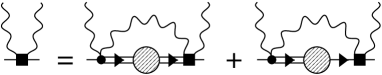
FIG. 2.: (a) Diagrammatic representation of the variance of the matrix $H$ in (1). (b) Representation of the second term of $J$ [Eq. (1)]. The random variables $V_{k}^{a}$ are denoted by wavy lines. (c) Shows the self-consistent equations determining the vertex $\,\,\hbox{\raisebox{-9.95845pt}{\psfig{width=14.22636pt}}}\,.$ There are three more such equations determining the three remaining vertices occuring in Fig. 1.

From $\langle G_{21}\rangle$ one obtains the density of states $d(z)$ in the usual fashion [7, 12, 13]. In order to make connection with the results discussed in [8], we specialize to the limit of small $m$. In this limit one obtains

$$d(0,y)\simeq\mbox{const.}+m/(4\pi y^{2})$$ (12)

for $m/(g+1)\leq 2y\leq m/(g-1)$ and zero otherwise, compare Eq. (108) in Ref. [5]. Here $2g=(\gamma+1/\gamma)$ and $z=x+{\rm i}y$ with $x,y$ real. We will analyze eigenvector correlations in the center $z_{0}$ of the support of the density of states, $z_{0}=x_{0}+{\rm i}y_{0}$ with $x_{0}=0$ and $y_{0}=m/(2g)$ where $d_{0}\equiv d(z_{0})\simeq g^{2}/(\pi m)$.

FIG. 3.: Vertex for calculating averages of products of Green functions in the limit of large $M,N$ with $M=mN$.

Eigenvector correlators. We make use of the relation

$$D(z_{1},z_{2})=\frac{1}{\pi^{2}}\frac{\partial}{\partial\overline{z}_{1}}\frac{\partial}{\partial z_{2}}F(z_{1},z_{2})$$ (13)

with

$$F(z_{1},z_{2})=\Big{\langle}N^{-1}\mbox{Tr}\,\big{[}(z_{1}-J)^{-1}\,(\overline{z}_{2}-J^{\dagger})^{-1}\big{]}\Big{\rangle}\,.$$ (14)

An expression for this average may be derived as described in [2]; cf. this reference for a diagrammatic representation of $F(z_{1},z_{2})$. The only difference between the case of interest here and the one discussed in Ref. [2] is that the vertex must be replaced by that shown in Fig. 3. The corresponding expression for $F(z_{1},z_{2})$ is valid in the limit of $M,N$ large, $M=mN$ and for $|z_{1}-z_{2}|^{2}>(\pi d(z_{+})\,N)^{-1}$ with $z_{+}=(z_{1}+z_{2})/2$.

Using Eq. (13) we obtain a (rather lengthy) expression for $O(z_{1},z_{2})$. To keep the formulae simple, we specialise further to the case where $z_{1}$ and $z_{2}$ are in the vicinity of $z_{0}$ and obtain to leading order in $m$ and lowest order in $|\delta z|$

$$O(z_{0},z_{0}+\delta z)\simeq-\left(\frac{m}{g^{2}}-\frac{m^{2}}{2g^{4}}\right)\frac{1}{\pi^{2}}\frac{1}{|\delta z|^{4}}\,.$$ (15)

Corrections breaking rotational invariance are of higher order. Comparison with Eq. (8) of Ref. [1] shows that locally, near the center of the support of the density of states, the eigenvector correlations for the ensemble (1) are the same as those in Ginibre’s ensemble, apart from an additional factor of $m/g^{2}-m^{2}/(2g^{4})$ which measures the strength of the non-Hermiticity in Eq. (1). According to Eq. (15), eigenvector correlations are strongest for $\gamma\simeq 1$, and vanish in the limit of $\gamma\rightarrow 0$ and $\gamma\rightarrow\infty$ which correspond to symmetric and complex symmetric $J$, respectively.

Given the expression (15), we may estimate $O(z_{0})$ up to a constant of order unity, in the way described in [2]. We obtain, to lowest order in $m$,

$$O(z_{0})\simeq N\frac{m}{g^{2}}$$ (16)

which is consistent with the result derived in [11]. In Fig. 4 we compare the expression (15) to the full result for $O(z_{1},z_{2})$ – as obtained within the self-consistent Born approximation – and observe very good agreement for $|\delta z|$ not too large.

Eq. (15) is valid to lowest order in $|\delta z|^{-1}$ and provided $|\delta z|^{2}>(\pi d_{0}N)^{-1}$. The behaviour of $O(z_{0},z_{0}+\delta z)$ for smaller values of $\delta z$ may be understood as follows. Assuming

$$O(z_{0},z_{0}+\delta z)\simeq\langle O_{\alpha\beta}\rangle\,R_{2}(z_{0},z_{0}+\delta z)$$ (17)

for $|\delta z|\simeq|\lambda_{\alpha}-\lambda_{\beta}|$ very small, one may estimate the two factors on the r.h.s. of this equation separately. First, if two eigenvalues $\lambda_{\alpha}$ and $\lambda_{\beta}$ of $J$ are very close to each other, one may argue that the corresponding overlap matrix element $O_{\alpha\beta}$ scales as $|\lambda_{\alpha}-\lambda_{\beta}|^{-2}$. This is seen by considering a $2\times 2$ matrix $J$ with arbitrary complex matrix elements $J_{kl}$. Denoting its right eigenvectors by $|R_{\alpha}\rangle=(1,\overline{\varrho}_{\alpha})^{\dagger}$, the corresponding left eigenvectors, assuming $\lambda_{1}\neq\lambda_{2}$ and subject to the condition (5) of biorthogonality, are given by by $\langle L_{1}|=(-\varrho_{2},1)/(\varrho_{1}-\varrho_{2})$ and $\langle L_{2}|=(-\varrho_{1},1)/(\varrho_{2}-\varrho_{1})$. Thus

$$O_{12} \equiv \langle L_{1}|L_{2}\rangle\langle R_{2}|R_{1}\rangle\propto-|\varrho_{1}-\varrho_{2}|^{-2}$$ (18)

$$\propto -|\lambda_{1}-\lambda_{2}|^{-2}\,.$$ (19)

For $\lambda_{\alpha}$ very close to $\lambda_{\beta}$ [namely on scales smaller than the mean level spacing $(\pi d_{0}N)^{-1/2}$] this behaviour pertains for arbitrary values of $N$. Second, the spectral two-point function scales as $R_{2}(z_{0},z_{0}+\delta z)\propto|\delta z|^{2}$ when $|\delta z|\rightarrow 0$ [8, 9]. Thus one concludes that $O(z_{1},z_{2})$ must converge to a constant as $|\delta z|$ approaches zero. Since the crossover from Eq. (15) to constant behaviour occurs at $|\delta z|^{2}\simeq(\pi d_{0}N)^{-1}$, one estimates, to lowest order in $m$

$$\frac{O(z_{0},z_{0}+\delta z)}{(d_{0}N)^{2}}\simeq\frac{m^{2}}{g}\qquad\mbox{for $|\delta z|^{2}\ll(\pi d_{0}N)^{-1}$}\,.$$ (20)

Eqs. (15) and (20) are consistent with the assumption that eigenvector correlations in the scattering ensemble (1) are universal in that $O(z_{0},z_{0}+\delta z)$ is given, after suitable rescaling and well within the support of the density of states, by the corresponding expression derived in Ref. [1] for Ginibre’s ensemble: defining [14] $\delta\tilde{z}\equiv\delta z\sqrt{\pi d_{0}N}$ one may expect, to lowest order in $m$

$$\frac{O(z_{0},z_{0}+\delta z)}{(d_{0}N)^{2}}$$ (22)

$$\simeq-\frac{m^{2}}{g}\frac{1}{|\delta\tilde{z}|^{4}}\,\left[1-(1+|\delta\tilde{z}|^{2})\,\exp(-|\delta\tilde{z}|^{2})\right]\,.$$

This expression interpolates between (15) and (20).

It must be pointed out that Eqs. (20) and (22) cannot be valid for very small values of $m=O(1/N)$, where the ensemble (1) deviates very little from the classical Gaussian unitary ensemble of random Hermitian matrices [10]. Spectral correlations in this situation have been analyzed in detail in Refs. [8, 15] where it was shown how the crossover from non-Hermitian to Hermitian ensembles may be characterized.

Numerical results. We have verified the validity of Eq. (22) using numerical simulations of of the ensemble (1), for $m=0.1$,$\gamma=0.5$ and $N=100,200,400,800$ and $1600$. Fig. 5 shows $O(z_{0},z_{0}+\delta z)/(d_{0}N)^{2}$ as a function of $\delta\tilde{z}$. We observe that the numerical results converge to Eqs. (22,15). Convergence with increasing values of $N$ is much faster for small values of $|\delta\tilde{z}|$ than for large values of $|\delta\tilde{z}|$. In fig. 5, the scale of the $x$-axis differs from that of fig. 4(a) and differences between (15) and the full result – as obtained within the self-consistent Born approximation – are not visible here.

We have also performed simulations for the modified ensemble (2). The results are very similar to those displayed in Fig. 5 (not shown).

 

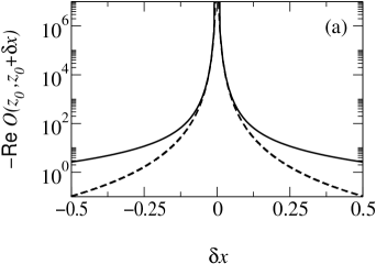
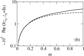
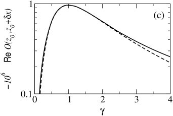
FIG. 4.: Shows ${\sf Re}O(z_{0},z_{0}+\delta x)$ as obtained within the self-consistent Born approximation (solid line) compared with the asymptotic expression (15) (dashed line) (a) as a function of $\delta x$ for $m=0.1$ and $\gamma=0.5$, (b) as a function of $m$ for $\delta x=0.01$ and $\gamma=0.5$, (c) as a function of $\gamma$ for $m=0.1$ and $\delta x=0.01$.

Conclusions. In this paper we have calculated the eigenvector correlator $O(z_{1},z_{2})$ for the ensemble (1) using the self-consistent Born approximation, and for both ensembles (1) and (2) using numerical simulations. Our results imply that eigenvector correlations in these ensembles are locally given by a universal law – after suitable rescaling of the complex energies. One may thus expect that local eigenvector correlations in more general ensembles (such as ensembles of random Fokker-Planck operators [12]) may be described by the law derived in [1]. It has been pointed out that such correlations may determine transient features in the dynamics of such systems [2]. The results found here may be of direct relevance for quantum scattering systems [6, 16].

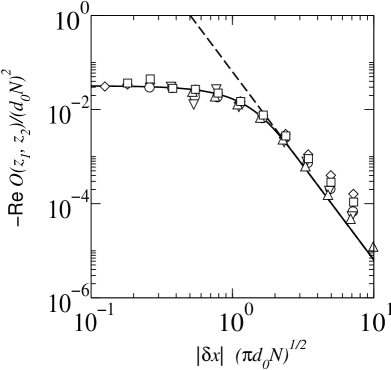
FIG. 5.: Shows ${\sf Re}\,O(z_{0},z_{0}+\delta x)/(d_{0}N)^{2}$ as a function of $\delta\widetilde{x}=\delta x\,\sqrt{\pi d_{0}N}$; for $m=0.1$,$\gamma=0.5$, $N=1600$ ($\triangle$), $N=800$ (), $N=400$ ($\circ$), $N=200$ ($\Box$) and $N=100$ ($\Diamond$). Also shown is the analytical estimate according to Eq. (15) (dashed line), and Eq. (22) (solid line).

REFERENCES

[1]
J. T. Chalker and B. Mehlig, Phys. Rev. Lett. 81, 3367 (1998).
[2]
B. Mehlig and J. T. Chalker, J. Math. Phys. (1999).
[3]
F. Haake et al., Z. Phys. B 88, 359 (1992).
[4] J. J. M. Verbaarschot, H.-A. Weidenmüller
and M. R. Zirnbauer, Phys. Rep. 129 367 (1985).
[5]
Y. Fyodorov and H.-J. Sommers, cond-mat/9701037 (unpublished);
J. Math. Phys. 38 1918 (1997).
[6] H.Schomerus et al., Physica A 278 469 (2000);
K.Frahm et al., Europhys. Lett. 49 , 48 (2000)
[7]
R. A. Janik et al., Nucl. Phys. B 498 313 (1997).
[8]
Y. Fyodorov and B. Khoruzenko, cond-mat/9903043 v2 (unpublished);
Phys. Rev. Lett. 83 65 (1999).
[9] Y. V. Fyodorov, private comnunication.
[10]
M. L. Mehta, Random Matrices and the Statistical Theory of Energy Levels
(Academic Press, New York, 1991).
[11]
R. A. Janik, W. Nörenberg, M. A. Nowak, G. Papp and I. Zahed,
Phys. Rev. E 60 2699 (1999).
[12]
J. T. Chalker and Z. J. Wang, Phys. Rev. Lett. 79, 1797 (1997);
Phys. Rev. E 61 196 (2000).
[13]
J. Feinberg and A. Zee, Nucl. Phys. B504, 579 (1997).
[14] This rescaling differs from that
used for the spectral
correlation function in Ref. [8] by a factor
of because in [8]
the case with fixed
was considered.
[15] Y. V. Fyodorov, B. A. Khoruzhenko and H.-J. Sommers,
Phys. Rev. Lett. 79 557 (1997).
[16] The relevance of eigenvector correlations
in quantum scattering systems is for instance discussed
in E. Persson, T. Gorin and I. Rotter,
Phys. Rev. E 54, 3339 (1996).