Generalized-Ensemble Algorithms for Molecular Simulations of Biopolymers

Ayori Mitsutake,^a,b Yuji Sugita,^a,b and Yuko Okamoto^a,b,

^aDepartment of Theoretical Studies

Institute for Molecular Science

Okazaki, Aichi 444-8585, Japan

and

^bDepartment of Functional Molecular Science

The Graduate University for Advanced Studies

Okazaki, Aichi 444-8585, Japan

Submitted to Biopolymers (Peptide Science)

Keywords: protein folding; generalized-ensemble algorithm; multicanonical algorithm;

simulated tempering; replica-exchange method; parallel tempering

ABSTRACT

In complex systems with many degrees of freedom such as peptides and proteins there exist a huge number of local-minimum-energy states. Conventional simulations in the canonical ensemble are of little use, because they tend to get trapped in states of these energy local minima. A simulation in generalized ensemble performs a random walk in potential energy space and can overcome this difficulty. From only one simulation run, one can obtain canonical-ensemble averages of physical quantities as functions of temperature by the single-histogram and/or multiple-histogram reweighting techniques. In this article we review uses of the generalized-ensemble algorithms. Three well-known methods, multicanonical algorithm, simulated tempering, and replica-exchange method, are described first. Both Monte Carlo and molecular dynamics versions of the algorithms are given. We then present three new generalized-ensemble algorithms which combine the merits of the above methods. The effectiveness of the methods for molecular simulations in the protein folding problem is tested with short peptide systems.

1 INTRODUCTION

Despite the great advancement of computer technology in the past decades, simulations of complex systems such as spin glasses and biopolymers are still greatly hampered by the multiple-minima problem. It is very difficult to obtain accurate canonical distributions at low temperatures by conventional Monte Carlo (MC) and molecular dynamics (MD) methods. This is because simulations at low temperatures tend to get trapped in one of huge number of local-minimum-energy states. The results thus will depend strongly on the initial conditions. One way to overcome this multiple-minima problem is to perform a simulation in a generalized ensemble where each state is weighted by a non-Boltzmann probability weight factor so that a random walk in potential energy space may be realized. The random walk allows the simulation to escape from any energy barrier and to sample much wider phase space than by conventional methods. Monitoring the energy in a single simulation run, one can obtain not only the global-minimum-energy state but also canonical ensemble averages as functions of temperature by the single-histogram [1] and/or multiple-histogram [2, 3] reweighting techniques (an extension of the multiple-histogram method is referred to as Weighted Histogram Analysis Method [3]).

One of the most well-known generalized-ensemble methods is perhaps multicanonical algorithm (MUCA) [4, 5] (for a recent review, see Ref. [6]). (The method is also referred to as entropic sampling [7] and adaptive umbrella sampling [8]. The mathematical equivalence of multicanonical algorithm and entropic sampling has been given in Ref. [9].) MUCA and its generalizations have been applied to spin glass systems (see, e.g., Refs. [10]–[13]). MUCA was also introduced to the molecular simulation field [14] (for previous reviews of generalized-ensemble approach in the protein folding problem, see, e.g., Refs. [15]–[17]). Since then MUCA has been extensively used in many applications in protein and related systems [18]–[44]. Molecular dynamics version of MUCA has also been developed [26, 27] (see also Refs. [45, 26] for Langevin dynamics version). Moreover, multidimensional (or multicomponent) extensions of MUCA can be found in Refs. [25, 29, 33].

While a simulation in multicanonical ensemble performs a free 1D random walk in energy space, that in simulated tempering (ST) [46, 47] (the method is also referred to as the method of expanded ensemble [46]) performs a free random walk in temperature space (for a review, see, e.g., Ref. [48]). This random walk, in turn, induces a random walk in potential energy space and allows the simulation to escape from states of energy local minima. ST has also been applied to protein folding problem [49]–[52].

A third generalized-ensemble algorithm that is related to MUCA is 1/k-sampling [53]. A simulation in 1/k-sampling performs a free random walk in entropy space, which, in turn, induces a random walk in potential energy space. The relation among the above three generalized-ensemble algorithms was discussed and the effectiveness of the three methods in protein folding problem was compared [51].

The generalized-ensemble method is powerful, but in the above three methods the probability weight factors are not a priori known and have to be determined by iterations of short trial simulations. This process can be non-trivial and very tedius for complex systems with many local-minimum-energy states. Therefore, there have been attempts to accelerate the convergence of the iterative process for MUCA [10, 25, 54, 55, 56, 8] (see also Ref. [6]).

A new generalized-ensemble algorithm that is based on the weight factor of Tsallis statistical mechanics [57] was recently developed with the hope of overcoming this difficulty [58, 59], and the method was applied to a peptide folding problem [60, 61]. A similar but slightly different formulation is given in Ref. [62]. See also Ref. [63] for a combination of Tsallis statistics with simulated tempering. (Optimization problems were also addressed by simulated annealing algorithms [64] based on the Tsallis weight in Refs. [65]–[67]. For reviews of molecular simulations based on Tsallis statistics, see, e.g., Refs. [68]–[70].) In this generalized ensemble the weight factor is known, once the value of the global-minimum energy is given [58]. The advantage of this ensemble is that it greatly simplifies the determination of the weight factor. However, the estimation of the global-minimum energy can still be very difficult.

In the replica-exchange method (REM) [71]–[73], the difficulty of weight factor determination is greatly alleviated. (A similar method was independently developed earlier in Ref. [74]. REM is also referred to as replica Monte Carlo method [74], multiple Markov chain method [75], and parallel tempering [48].) In this method, a number of non-interacting copies of the original system (or replicas) at different temperatures are simulated independently and simultaneously by the conventional MC or MD method. Every few steps, pairs of replicas are exchanged with a specified transition probability. The weight factor is just the product of Boltzmann factors, and so it is essentially known.

REM has already been used in many applications in protein systems [76, 77, 52, 78, 79, 80, 81]. Systems of Lennard-Jones particles have also been studied by this method in various ensembles [82]–[85]. Moreover, REM was applied to cluster studies in quantum chemistry field [86]. The details of molecular dynamics algorithm have been worked out for REM [78] (see also Refs. [76, 87]). We then developed a multidimensional REM which is particularly useful in free energy calculations [80] (see also Refs. [88, 82, 89]).

However, REM also has a computational difficulty: As the number of degrees of freedom of the system increases, the required number of replicas also greatly increases, whereas only a single replica is simulated in MUCA or ST. This demands a lot of computer power for complex systems. Our solution to this problem is: Use REM for the weight factor determinations of MUCA or ST, which is much simpler than previous iterative methods of weight determinations, and then perform a long MUCA or ST production run. The first example is the replica-exchange multicanonical algorithm (REMUCA) [90]. In REMUCA, a short replica-exchange simulation is performed, and the multicanonical weight factor is determined by the multiple-histogram reweighting techniques [2, 3]. Another example of such a combination is the replica-exchange simulated tempering (REST) [91]. In REST, a short replica-exchange simulation is performed, and the simulated tempering weight factor is determined by the multiple-histogram reweighting techniques [2, 3].

We have introduced a further extension of REMUCA, which we refer to as multicanonical replica-exchange method (MUCAREM) [90]. In MUCAREM, the multicanonical weight factor is first determined as in REMUCA, and then a replica-exchange multicanonical production simulation is performed with a small number of replicas.

In this article, we describe the six generalized-ensemble algorithms mentioned above. Namely, we first review three familiar methods: MUCA, ST, and REM. We then present the three new algorithms: REMUCA, REST, and MUCAREM. The effectiveness of these methods is tested with short peptide systems.

2 GENERALIZED-ENSEMBLE ALGORITHMS

2.1 Multicanonical Algorithm and Simulated Tempering

Let us consider a system of $N$ atoms of mass $m_{k}$ ($k=1,\cdots,N$) with their coordinate vectors and momentum vectors denoted by $q\equiv\{{\mbox{\boldmath$q$}}_{1},\cdots,{\mbox{\boldmath$q$}}_{N}\}$ and $p\equiv\{{\mbox{\boldmath$p$}}_{1},\cdots,{\mbox{\boldmath$p$}}_{N}\}$, respectively. The Hamiltonian $H(q,p)$ of the system is the sum of the kinetic energy $K(p)$ and the potential energy $E(q)$:

$$H(q,p)=K(p)+E(q)~{},$$ (1)

where

$$K(p)=\sum_{k=1}^{N}\frac{{\mbox{\boldmath$p$}_{k}}^{2}}{2m_{k}}~{}.$$ (2)

In the canonical ensemble at temperature $T$ each state $x\equiv(q,p)$ with the Hamiltonian $H(q,p)$ is weighted by the Boltzmann factor:

$$W_{\rm B}(x;T)=e^{-\beta H(q,p)}~{},$$ (3)

where the inverse temperature $\beta$ is defined by $\beta=1/k_{\rm B}T$ ($k_{\rm B}$ is the Boltzmann constant). The average kinetic energy at temperature $T$ is then given by

$$\left<~{}K(p)~{}\right>_{T}=\left<\sum_{k=1}^{N}\frac{{\mbox{\boldmath$p$}_{k}}^{2}}{2m_{k}}\right>_{T}=\frac{3}{2}Nk_{\rm B}T~{}.$$ (4)

Because the coordinates $q$ and momenta $p$ are decoupled in Eq. (1), we can suppress the kinetic energy part and can write the Boltzmann factor as

$$W_{\rm B}(x;T)=W_{\rm B}(E;T)=e^{-\beta E}~{}.$$ (5)

The canonical probability distribution of potential energy $P_{\rm B}(E;T)$ is then given by the product of the density of states $n(E)$ and the Boltzmann weight factor $W_{\rm B}(E;T)$:

$$P_{\rm B}(E;T)\propto n(E)W_{\rm B}(E;T)~{}.$$ (6)

Since $n(E)$ is a rapidly increasing function and the Boltzmann factor decreases exponentially, the canonical ensemble yields a bell-shaped distribution which has a maximum around the average energy at temperature $T$. The conventional MC or MD simulations at constant temperature are expected to yield $P_{\rm B}(E;T)$, but, in practice, it is very difficult to obtain accurate canonical distributions of complex systems at low temperatures by conventional simulation methods. This is because simulations at low temperatures tend to get trapped in one or a few of local-minimum-energy states.

In the multicanonical ensemble (MUCA) [4, 5], on the other hand, each state is weighted by a non-Boltzmann weight factor $W_{\rm mu}(E)$ (which we refer to as the multicanonical weight factor) so that a uniform energy distribution $P_{\rm mu}(E)$ is obtained:

$$P_{\rm mu}(E)\propto n(E)W_{\rm mu}(E)\equiv{\rm constant}.$$ (7)

The flat distribution implies that a free random walk in the potential energy space is realized in this ensemble. This allows the simulation to escape from any local minimum-energy states and to sample the configurational space much more widely than the conventional canonical MC or MD methods.

From the definition in Eq. (7) the multicanonical weight factor is inversely proportional to the density of states, and we can write it as follows:

$$W_{\rm mu}(E)\equiv e^{-\beta_{0}E_{\rm mu}(E;T_{0})}=\frac{1}{n(E)}~{},$$ (8)

where we have chosen an arbitrary reference temperature, $T_{0}=1/k_{\rm B}\beta_{0}$, and the “multicanonical potential energy” is defined by

$$E_{\rm mu}(E;T_{0})=k_{\rm B}T_{0}\ln n(E)=T_{0}S(E)~{}.$$ (9)

Here, $S(E)$ is the entropy in the microcanonical ensemble. Since the density of states of the system is usually unknown, the multicanonical weight factor has to be determined numerically by iterations of short preliminary runs [4, 5] as described in detail below.

A multicanonical Monte Carlo simulation is performed, for instance, with the usual Metropolis criterion [92]: The transition probability of state $x$ with potential energy $E$ to state $x^{\prime}$ with potential energy $E^{\prime}$ is given by

$$w(x\rightarrow x^{\prime})=\left\{\begin{array}[]{ll}1~{},&{\rm for}\ \Delta E_{\rm mu}\leq 0~{},\cr\exp\left(-\beta_{0}\Delta E_{\rm mu}\right)~{},&{\rm for}\ \Delta E_{\rm mu}>0~{},\end{array}\right.$$ (10)

where

$$\Delta E_{\rm mu}\equiv E_{\rm mu}(E^{\prime};T_{0})-E_{\rm mu}(E;T_{0})~{}.$$ (11)

The molecular dynamics algorithm in multicanonical ensemble also naturally follows from Eq. (8), in which the regular constant temperature molecular dynamics simulation (with $T=T_{0}$) is performed by solving the following modified Newton equation: [26, 27]

$$\dot{{\mbox{\boldmath$p$}}}_{k}~{}=~{}-\frac{\partial E_{\rm mu}(E;T_{0})}{\partial{\mbox{\boldmath$q$}}_{k}}~{}=~{}\frac{\partial E_{\rm mu}(E;T_{0})}{\partial E}~{}{\mbox{\boldmath$f$}}_{k}~{},$$ (12)

where ${\mbox{\boldmath$f$}}_{k}$ is the usual force acting on the $k$-th atom ($k=1,\cdots,N$). From Eq. (9) this equation can be rewritten as

$$\dot{{\mbox{\boldmath$p$}}}_{k}~{}=~{}\frac{T_{0}}{T(E)}~{}{\mbox{\boldmath$f$}}_{k}~{},$$ (13)

where the following thermodynamic relation gives the definition of the “effective temperature” $T(E)$:

$$\left.\frac{\partial S(E)}{\partial E}\right|_{E=E_{a}}~{}=~{}\frac{1}{T(E_{a})}~{},$$ (14)

with

$$E_{a}~{}=~{}<E>_{T(E_{a})}~{}.$$ (15)

The multicanonical weight factor is usually determined by iterations of short trial simulations. The details of this process are described, for instance, in Refs. [10, 21]. For the first run, a canonical simulation at a sufficiently high temperature $T_{0}$ is performed, i.e., we set

$$\left\{\begin{array}[]{rl}E^{(1)}_{\rm mu}(E;T_{0})&=~{}E~{},\\ W^{(1)}_{\rm mu}(E;T_{0})&=~{}W_{\rm B}(E;T_{0})~{}=~{}\exp\left(-\beta_{0}E\right)~{}.\end{array}\right.$$ (16)

We define the maximum energy value $E_{\rm max}$ under which we want to have a flat energy distribution by the average potential energy at temperature $T_{0}$:

$$E_{\rm max}=<E>_{T_{0}}~{}.$$ (17)

Above $E_{\rm max}$ we have the canonical distribution at $T=T_{0}$. In the $\ell$-th iteration a simulation with the weight $W^{(\ell)}_{\rm mu}(E;T_{0})=\exp\left(-\beta_{0}E^{(\ell)}_{\rm mu}(E;T_{0})\right)$ is performed, and the histogram $N^{(\ell)}(E)$ of the potential energy distribution $P^{(\ell)}_{\rm mu}(E)$ is obtained. Let $E^{(\ell)}_{\rm min}$ be the lowest-energy value that was obtained throughout the preceding iterations including the present simulation. The multicanonical weight factor for the $(\ell+1)$-th iteration is then given by

$$E^{(\ell+1)}_{\rm mu}(E;T_{0})=\left\{\begin{array}[]{@{\,}ll}E~{},&\mbox{for $E\geq E_{\rm max}$,}\\ E^{(\ell)}_{\rm mu}(E;T_{0})+k_{\rm B}T_{0}\ln N^{(\ell)}(E)-c^{(\ell)}~{},&\mbox{for $E^{(\ell)}_{\rm min}\leq E<E_{\rm max}$,}\\ \left.\displaystyle{\frac{\partial E^{(\ell+1)}_{\rm mu}(E;T_{0})}{\partial E}}\right|_{E=E^{(\ell)}_{\rm min}}\left(E-E^{(\ell)}_{\rm min}\right)+E^{(\ell+1)}_{\rm mu}(E^{(\ell)}_{\rm min};T_{0}),&\mbox{for $E<E^{(\ell)}_{\rm min}$,}\end{array}\right.$$ (18)

where the constant $c^{(\ell)}$ is introduced to ensure the continuity at $E=E_{\rm max}$ and we have

$$c^{(\ell)}=k_{\rm B}T_{0}\ln N^{(\ell)}(E_{\rm max})~{}.$$ (19)

We iterate this process until the obtained energy distribution becomes reasonably flat, say, of the same order of magnitude, for $E<E_{\rm max}$. When the convergence is reached, we should have that $E^{(\ell)}_{\rm min}$ is equal to the global-minimum potential energy value.

It is also common especially when working in MD algorithm to use polynomials and other smooth functions to fit the histograms during the iterations [22, 27, 8]. We have shown that the cubic spline functions work well [90].

However, the iterative process can be non-trivial and very tedius for complex systems, and there have been attempts to accelerate the convergence of the iterative process [10, 25, 54, 55, 56, 8].

After the optimal multicanonical weight factor is determined, one performs a long multicanonical simulation once. By monitoring the potential energy throughout the simulation, one can find the global-minimum-energy state. Moreover, by using the obtained histogram $N_{\rm mu}(E)$ of the potential energy distribution $P_{\rm mu}(E)$ the expectation value of a physical quantity $A$ at any temperature $T=1/k_{\rm B}\beta$ is calculated from

$$<A>_{T}\ =\frac{\displaystyle{\sum_{E}~{}A(E)~{}n(E)~{}e^{-\beta E}}}{\displaystyle{\sum_{E}~{}n(E)~{}e^{-\beta E}}}~{},$$ (20)

where the best estimate of the density of states is given by the single-histogram reweighting techniques (see Eq. (7)) [1]:

$$n(E)=\frac{N_{\rm mu}(E)}{W_{\rm mu}(E)}~{}.$$ (21)

In the numerical work, we want to avoid round-off errors (and overflows and underflows) as much as possible. It is usually better to combine exponentials as follows (see Eq. (8)):

$$<A>_{T}\ =\frac{\displaystyle{\sum_{E}~{}A(E)~{}N_{\rm mu}(E)~{}e^{\beta_{0}E_{\rm mu}(E;T_{0})-\beta E}}}{\displaystyle{\sum_{E}~{}N_{\rm mu}(E)~{}e^{\beta_{0}E_{\rm mu}(E;T_{0})-\beta E}}}~{}.$$ (22)

We now briefly review the original simulated tempering (ST) method [46, 47]. In this method temperature itself becomes a dynamical variable, and both the configuration and the temperature are updated during the simulation with a weight:

$$W_{\rm ST}(E;T)=e^{-\beta E+a(T)}~{},$$ (23)

where the function $a(T)$ is chosen so that the probability distribution of temperature is flat:

$$P_{\rm ST}(T)=\int dE~{}n(E)~{}W_{{\rm ST}}(E;T)=\int dE~{}n(E)~{}e^{-\beta E+a(T)}={\rm constant}~{}.$$ (24)

Hence, in simulated tempering the temperature is sampled uniformly. A free random walk in temperature space is realized, which in turn induces a random walk in potential energy space and allows the simulation to escape from states of energy local minima.

In the numerical work we discretize the temperature in $M$ different values, $T_{m}$ ($m=1,\cdots,M$). Without loss of generality we can order the temperature so that $T_{1}<T_{2}<\cdots<T_{M}$. The lowest temperature $T_{1}$ should be sufficiently low so that the simulation can explore the global-minimum-energy region, and the highest temperature $T_{M}$ should be sufficiently high so that no trapping in an energy-local-minimum state occurs. The probability weight factor in Eq. (23) is now written as

$$W_{\rm ST}(E;T_{m})=e^{-\beta_{m}E+a_{m}}~{},$$ (25)

where $a_{m}=a(T_{m})$ ($m=1,\cdots,M$). The parameters $a_{m}$ are not known a priori and have to be determined by iterations of short simulations. This process can be non-trivial and very difficult for complex systems. Note that from Eqs. (24) and (25) we have

$$e^{-a_{m}}\propto\int dE~{}n(E)~{}e^{-\beta_{m}E}~{}.$$ (26)

The parameters $a_{m}$ are therefore “dimensionless” Helmholtz free energy at temperature $T_{m}$ (i.e., the inverse temperature $\beta_{m}$ multiplied by the Helmholtz free energy).

Once the parameters $a_{m}$ are determined and the initial configuration and the initial temperature $T_{m}$ are chosen, a simulated tempering simulation is then realized by alternately performing the following two steps [46, 47]:

1. A canonical MC or MD simulation at the fixed temperature $T_{m}$ is carried out for a certain MC or MD steps.

2. The temperature $T_{m}$ is updated to the neighboring values $T_{m\pm 1}$ with the configuration fixed. The transition probability of this temperature-updating process is given by the Metropolis criterion (see Eq. (25)):

   $$w(T_{m}\rightarrow T_{m\pm 1})=\left\{\begin{array}[]{ll}1~{},&{\rm for}\ \Delta\leq 0~{},\cr\exp\left(-\Delta\right)~{},&{\rm for}\ \Delta>0~{},\end{array}\right.$$ (27)

   where

   $$\Delta=\left(\beta_{m\pm 1}-\beta_{m}\right)E-\left(a_{m\pm 1}-a_{m}\right)~{}.$$ (28)

Note that in Step 2 we exchange only pairs of neighboring temperatures in order to secure sufficiently large acceptance ratio of temperature updates.

As in multicanonical algorithm, the simulated tempering parameters $a_{m}=a(T_{m})$ ($m=1,\cdots,M$) are also determined by iterations of short trial simulations (see, e.g., Refs. [48, 49, 51] for details). Here, we give the one in Ref. [51].

During the trial simulations we keep track of the temperature distribution as a histogram $N_{m}=N(T_{m})$ ($m=1,\cdots,M$).

1. Start with a short canonical simulation (i.e., $a_{m}=0$) updating only configurations at temperature $T_{m}=T_{M}$ (we initially set the temperature label $m$ to $M$) and calculate the average potential energy $<E>_{T_{M}}$. Here, the histogram $N_{n}$ will have non-zero entry only for $n=m=M$.

2. Calculate new parameters $a_{n}$ according to

   $$a_{n}=\left\{\begin{array}[]{ll}a_{n}-\ln N_{n}~{},&{\rm for}~{}~{}m\leq n\leq M~{},\cr a_{n}-<E>_{T_{m}}\left(\beta_{m-1}-\beta_{m}\right)~{},&{\rm for}~{}~{}n=m-1~{},\cr-\infty~{},&{\rm for}~{}~{}n<m-1~{}.\end{array}\right.$$ (29)

   This weight implies that the temperature will range between $T_{m-1}$ and $T_{M}$.

3. Start a new simulation, now updating both configurations and temperatures, with weight $W_{\rm ST}(E;T_{n})=e^{-\beta_{n}E+a_{n}}$ and sample the distribution of temperatures $T_{n}$ in the histogram $N_{n}=N(T_{n})$. For $T=T_{m-1}$ calculate the average potential energy $<E>_{T_{m-1}}$.

4. If the histogram $N_{n}$ is approximately flat in the temperature range $T_{m-1}\leq T_{n}\leq T_{M}$, set $m=m-1$. Otherwise, leave $m$ unchanged.

5. Iterate the last three steps until the obtained temperature distribution $N_{n}$ becomes flat over the whole temperature range $\left[T_{1},T_{M}\right]$.

After the optimal simulated tempering weight factor is determined, one performs a long simulated tempering run once. From the results of this production run, one can obtain the canonical ensemble average of a physical quantity $A$ as a function of temperature from Eq. (20), where the density of states is given by the multiple-histogram reweighting techniques [2, 3] as follows. Let $N_{m}(E)$ and $n_{m}$ be respectively the potential-energy histogram and the total number of samples obtained at temperature $T_{m}=1/k_{\rm B}\beta_{m}$ ($m=1,\cdots,M$). The best estimate of the density of states is then given by [2, 3]

$$n(E)=\frac{\displaystyle{\sum_{m=1}^{M}~{}g_{m}^{-1}~{}N_{m}(E)}}{\displaystyle{\sum_{m=1}^{M}~{}g_{m}^{-1}~{}n_{m}~{}e^{f_{m}-\beta_{m}E}}}~{},$$ (30)

where

$$e^{-f_{m}}=\sum_{E}~{}n(E)~{}e^{-\beta_{m}E}~{}.$$ (31)

Here, $g_{m}=1+2\tau_{m}$, and $\tau_{m}$ is the integrated autocorrelation time at temperature $T_{m}$. Note that Eqs. (30) and (31) are solved self-consistently by iteration [2, 3] to obtain the dimensionless Helmholtz free energy $f_{m}$ (and the density of states $n(E)$). We remark that in the numeraical work, it is often more stable to use the following equations instead of Eqs. (30) and (31):

$$P_{\rm B}(E;T)=n(E)e^{-\beta E}=\frac{\displaystyle{\sum_{m=1}^{M}~{}g_{m}^{-1}~{}N_{m}(E)}}{\displaystyle{\sum_{m=1}^{M}~{}g_{m}^{-1}~{}n_{m}~{}e^{f_{m}-(\beta_{m}-\beta)E}}}~{},$$ (32)

where

$$e^{-f_{m}}=\sum_{E}~{}P_{\rm B}(E;T_{m})~{}.$$ (33)

The equations are solved iteratively as follows. We can set all the $f_{m}$ ($m=1,\cdots,M$) to, e.g., zero initially. We then use Eq. (32) to obtain $P_{\rm B}(E;T_{m})$ ($m=1,\cdots,M$), which are substituted into Eq. (33) to obtain next values of $f_{m}$, and so on.

2.2 Replica-Exchange Method

The replica-exchange method (REM) [71]–[74] was developed as an extension of simulated tempering [71] (thus it is also referred to as parallel tempering [48]) (see, e.g., Ref. [78] for a detailed description of the algorithm). The system for REM consists of $M$ non-interacting copies (or, replicas) of the original system in the canonical ensemble at $M$ different temperatures $T_{m}$ ($m=1,\cdots,M$). We arrange the replicas so that there is always exactly one replica at each temperature. Then there is a one-to-one correspondence between replicas and temperatures; the label $i$ ($i=1,\cdots,M$) for replicas is a permutation of the label $m$ ($m=1,\cdots,M$) for temperatures, and vice versa:

$$\left\{\begin{array}[]{rl}i&=~{}i(m)~{}\equiv~{}f(m)~{},\cr m&=~{}m(i)~{}\equiv~{}f^{-1}(i)~{},\end{array}\right.$$ (34)

where $f(m)$ is a permutation function of $m$ and $f^{-1}(i)$ is its inverse.

Let $X=\left\{x_{1}^{[i(1)]},\cdots,x_{M}^{[i(M)]}\right\}=\left\{x_{m(1)}^{[1]},\cdots,x_{m(M)}^{[M]}\right\}$ stand for a “state” in this generalized ensemble. The state $X$ is specified by the $M$ sets of coordinates $q^{[i]}$ and momenta $p^{[i]}$ of $N$ atoms in replica $i$ at temperature $T_{m}$:

$$x_{m}^{[i]}\equiv\left(q^{[i]},p^{[i]}\right)_{m}~{}.$$ (35)

Because the replicas are non-interacting, the weight factor for the state $X$ in this generalized ensemble is given by the product of Boltzmann factors for each replica (or at each temperature):

$$W_{\rm REM}(X)=\exp\left\{-\displaystyle{\sum_{i=1}^{M}\beta_{m(i)}H\left(q^{[i]},p^{[i]}\right)}\right\}=\exp\left\{-\displaystyle{\sum_{m=1}^{M}\beta_{m}H\left(q^{[i(m)]},p^{[i(m)]}\right)}\right\}~{},$$ (36)

where $i(m)$ and $m(i)$ are the permutation functions in Eq. (34).

We now consider exchanging a pair of replicas in the generalized ensemble. Suppose we exchange replicas $i$ and $j$ which are at temperatures $T_{m}$ and $T_{n}$, respectively:

$$X=\left\{\cdots,x_{m}^{[i]},\cdots,x_{n}^{[j]},\cdots\right\}\longrightarrow\ X^{\prime}=\left\{\cdots,x_{m}^{[j]\prime},\cdots,x_{n}^{[i]\prime},\cdots\right\}~{}.$$ (37)

Here, $i$, $j$, $m$, and $n$ are related by the permutation functions in Eq. (34), and the exchange of replicas introduces a new permutation function $f^{\prime}$:

$$\left\{\begin{array}[]{rl}i&=f(m)\longrightarrow j=f^{\prime}(m)~{},\cr j&=f(n)\longrightarrow i=f^{\prime}(n)~{}.\cr\end{array}\right.$$ (38)

The exchange of replicas can be written in more detail as

$$\left\{\begin{array}[]{rl}x_{m}^{[i]}\equiv\left(q^{[i]},p^{[i]}\right)_{m}&\longrightarrow\ x_{m}^{[j]\prime}\equiv\left(q^{[j]},p^{[j]\prime}\right)_{m}~{},\cr x_{n}^{[j]}\equiv\left(q^{[j]},p^{[j]}\right)_{n}&\longrightarrow\ x_{n}^{[i]\prime}\equiv\left(q^{[i]},p^{[i]\prime}\right)_{n}~{},\end{array}\right.$$ (39)

where the definitions for $p^{[i]\prime}$ and $p^{[j]\prime}$ will be given below. We remark that this process is equivalent to exchanging a pair of temperatures $T_{m}$ and $T_{n}$ for the corresponding replicas $i$ and $j$ as follows:

$$\left\{\begin{array}[]{rl}x_{m}^{[i]}\equiv\left(q^{[i]},p^{[i]}\right)_{m}&\longrightarrow\ x_{n}^{[i]\prime}\equiv\left(q^{[i]},p^{[i]\prime}\right)_{n}~{},\cr x_{n}^{[j]}\equiv\left(q^{[j]},p^{[j]}\right)_{n}&\longrightarrow\ x_{m}^{[j]\prime}\equiv\left(q^{[j]},p^{[j]\prime}\right)_{m}~{}.\end{array}\right.$$ (40)

In the original implementation of the replica-exchange method (REM) [71]–[74], Monte Carlo algorithm was used, and only the coordinates $q$ (and the potential energy function $E(q)$) had to be taken into account. In molecular dynamics algorithm, on the other hand, we also have to deal with the momenta $p$. We proposed the following momentum assignment in Eq. (39) (and in Eq. (40)) [78]:

$$\left\{\begin{array}[]{rl}p^{[i]\prime}&\equiv\displaystyle{\sqrt{\frac{T_{n}}{T_{m}}}}~{}p^{[i]}~{},\cr p^{[j]\prime}&\equiv\displaystyle{\sqrt{\frac{T_{m}}{T_{n}}}}~{}p^{[j]}~{},\end{array}\right.$$ (41)

which we believe is the simplest and the most natural. This assignment means that we just rescale uniformly the velocities of all the atoms in the replicas by the square root of the ratio of the two temperatures so that the temperature condition in Eq. (4) may be satisfied.

In order for this exchange process to converge towards an equilibrium distribution, it is sufficient to impose the detailed balance condition on the transition probability $w(X\rightarrow X^{\prime})$:

$$W_{\rm REM}(X)\ w(X\rightarrow X^{\prime})=W_{\rm REM}(X^{\prime})\ w(X^{\prime}\rightarrow X)~{}.$$ (42)

From Eqs. (1), (2), (36), (41), and (42), we have

$$\begin{array}[]{rl}\displaystyle{\frac{w(X\rightarrow X^{\prime})}{w(X^{\prime}\rightarrow X)}}&=\exp\left\{-\beta_{m}\left[K\left(p^{[j]\prime}\right)+E\left(q^{[j]}\right)\right]-\beta_{n}\left[K\left(p^{[i]\prime}\right)+E\left(q^{[i]}\right)\right]\right.\cr&\ \ \ \ \ \ \ \ \ \ \left.+\beta_{m}\left[K\left(p^{[i]}\right)+E\left(q^{[i]}\right)\right]+\beta_{n}\left[K\left(p^{[j]}\right)+E\left(q^{[j]}\right)\right]\right\}~{},\cr&=\exp\left\{-\beta_{m}\displaystyle{\frac{T_{m}}{T_{n}}}K\left(p^{[j]}\right)-\beta_{n}\displaystyle{\frac{T_{n}}{T_{m}}}K\left(p^{[i]}\right)+\beta_{m}K\left(p^{[i]}\right)+\beta_{n}K\left(p^{[j]}\right)\right.\cr&\ \ \ \ \ \ \ \ \ \ \left.-\beta_{m}\left[E\left(q^{[j]}\right)-E\left(q^{[i]}\right)\right]-\beta_{n}\left[E\left(q^{[i]}\right)-E\left(q^{[j]}\right)\right]\right\}~{},\cr&=\exp\left(-\Delta\right)~{},\end{array}$$ (43)

where

$$\Delta\equiv\left(\beta_{n}-\beta_{m}\right)\left(E\left(q^{[i]}\right)-E\left(q^{[j]}\right)\right)~{},$$ (44)

and $i$, $j$, $m$, and $n$ are related by the permutation functions (in Eq. (34)) before the exchange:

$$\left\{\begin{array}[]{ll}i&=f(m)~{},\cr j&=f(n)~{}.\end{array}\right.$$ (45)

This can be satisfied, for instance, by the usual Metropolis criterion [92]:

$$w(X\rightarrow X^{\prime})\equiv w\left(x_{m}^{[i]}~{}\left|~{}x_{n}^{[j]}\right.\right)=\left\{\begin{array}[]{ll}1~{},&{\rm for}\ \Delta\leq 0~{},\cr\exp\left(-\Delta\right)~{},&{\rm for}\ \Delta>0~{},\end{array}\right.$$ (46)

where in the second expression (i.e., $w(x_{m}^{[i]}|x_{n}^{[j]})$) we explicitly wrote the pair of replicas (and temperatures) to be exchanged. Note that this is exactly the same criterion that was originally derived for Monte Carlo algorithm [71]–[74].

Without loss of generality we can again assume $T_{1}<T_{2}<\cdots<T_{M}$. A simulation of the replica-exchange method (REM) [71]–[74] is then realized by alternately performing the following two steps:

1. Each replica in canonical ensemble of the fixed temperature is simulated $simultaneously$ and $independently$ for a certain MC or MD steps.

2. A pair of replicas at neighboring temperatures, say $x_{m}^{[i]}$ and $x_{m+1}^{[j]}$, are exchanged with the probability $w\left(x_{m}^{[i]}~{}\left|~{}x_{m+1}^{[j]}\right.\right)$ in Eq. (46).

Note that in Step 2 we exchange only pairs of replicas corresponding to neighboring temperatures, because the acceptance ratio of the exchange decreases exponentially with the difference of the two $\beta$’s (see Eqs. (44) and (46)). Note also that whenever a replica exchange is accepted in Step 2, the permutation functions in Eq. (34) are updated.

The REM simulation is particularly suitable for parallel computers. Because one can minimize the amount of information exchanged among nodes, it is best to assign each replica to each node (exchanging pairs of temperature values among nodes is much faster than exchanging coordinates and momenta). This means that we keep track of the permutation function $m(i;t)=f^{-1}(i;t)$ in Eq. (34) as a function of MC or MD step $t$ during the simulation. After parallel canonical MC or MD simulations for a certain steps (Step 1), $M/2$ pairs of replicas corresponding to neighboring temperatures are simulateneously exchanged (Step 2), and the pairing is alternated between the two possible choices, i.e., ($T_{1},T_{2}$), ($T_{3},T_{4}$), $\cdots$ and ($T_{2},T_{3}$), ($T_{4},T_{5}$), $\cdots$.

The major advantage of REM over other generalized-ensemble methods such as multicanonical algorithm [4, 5] and simulated tempering [46, 47] lies in the fact that the weight factor is a priori known (see Eq. (36)), while in the latter algorithms the determination of the weight factors can be very tedius and time-consuming. A random walk in “temperature space” is realized for each replica, which in turn induces a random walk in potential energy space. This alleviates the problem of getting trapped in states of energy local minima. In REM, however, the number of required replicas increases as the system size $N$ increases (according to $\sqrt{N}$) [71]. This demands a lot of computer power for complex systems.

2.3 Replica-Exchange Multicanonical Algorithm and Replica-Exchange Simulated Tempering

The replica-exchange multicanonical algorithm (REMUCA) [90] overcomes both the difficulties of MUCA (the multicanonical weight factor determination is non-trivial) and REM (a lot of replicas, or computation time, is required). In REMUCA we first perform a short REM simulation (with $M$ replicas) to determine the multicanonical weight factor and then perform with this weight factor a regular multicanonical simulation with high statistics. The first step is accomplished by the multiple-histogram reweighting techniques [2, 3]. Let $N_{m}(E)$ and $n_{m}$ be respectively the potential-energy histogram and the total number of samples obtained at temperature $T_{m}=1/k_{\rm B}\beta_{m}$ of the REM run. The density of states $n(E)$ is then given by solving Eqs. (30) and (31) self-consistently by iteration [2, 3].

Once the estimate of the density of states is obtained, the multicanonical weight factor can be directly determined from Eq. (8) (see also Eq. (9)). Actually, the multicanonical potential energy, $E_{\rm mu}(E;T_{0})$, thus determined is only reliable in the following range:

$$E_{1}\leq E\leq E_{M}~{},$$ (47)

where

$$\left\{\begin{array}[]{rl}E_{1}&=~{}<E>_{T_{1}}~{},\\ E_{M}&=~{}<E>_{T_{M}}~{},\end{array}\right.$$ (48)

and $T_{1}$ and $T_{M}$ are respectively the lowest and the highest temperatures used in the REM run. Outside this range we extrapolate the multicanonical potential energy linearly:

$${\cal E}_{\rm mu}^{\{0\}}(E)\equiv\left\{\begin{array}[]{@{\,}ll}\left.\displaystyle{\frac{\partial E_{\rm mu}(E;T_{0})}{\partial E}}\right|_{E=E_{1}}(E-E_{1})+E_{\rm mu}(E_{1};T_{0})~{},&\mbox{for $E<E_{1}$,}\\ E_{\rm mu}(E;T_{0})~{},&\mbox{for $E_{1}\leq E\leq E_{M}$,}\\ \left.\displaystyle{\frac{\partial E_{\rm mu}(E;T_{0})}{\partial E}}\right|_{E=E_{M}}(E-E_{M})+E_{\rm mu}(E_{M};T_{0})~{},&\mbox{for $E>E_{M}$.}\end{array}\right.$$ (49)

The multicanonical MC and MD runs are then performed with the Metropolis criterion of Eq. (10) and with the Newton equation in Eq. (12), respectively, in which ${\cal E}_{\rm mu}^{\{0\}}(E)$ in Eq. (49) is substituted into $E_{\rm mu}(E;T_{0})$. We expect to obtain a flat potential energy distribution in the range of Eq. (47). Finally, the results are analyzed by the single-histogram reweighting techniques as described in Eq. (21) (and Eq. (20)).

Some remarks are now in order. From Eqs. (9), (14), (15), and (48), Eq. (49) becomes

$${\cal E}_{\rm mu}^{\{0\}}(E)=\left\{\begin{array}[]{@{\,}ll}\displaystyle{\frac{T_{0}}{T_{1}}}(E-E_{1})+T_{0}S(E_{1})=\displaystyle{\frac{T_{0}}{T_{1}}}E+{\rm constant}~{},&\mbox{for $E<E_{1}\equiv<E>_{T_{1}}$,}\\ T_{0}S(E)~{},&\mbox{for $E_{1}\leq E\leq E_{M}$,}\\ \displaystyle{\frac{T_{0}}{T_{M}}}(E-E_{M})+T_{0}S(E_{M})=\displaystyle{\frac{T_{0}}{T_{M}}}E+{\rm constant}~{},&\mbox{for $E>E_{M}\equiv<E>_{T_{M}}$.}\end{array}\right.$$ (50)

The Newton equation in Eq. (12) is then written as (see Eqs. (eqn9b), (14), and (15))

$$\dot{{\mbox{\boldmath$p$}}}_{k}=\left\{\begin{array}[]{@{\,}ll}\displaystyle{\frac{T_{0}}{T_{1}}}~{}{\mbox{\boldmath$f$}}_{k}~{},&\mbox{for $E<E_{1}$,}\\ \displaystyle{\frac{T_{0}}{T(E)}}~{}{\mbox{\boldmath$f$}}_{k}~{},&\mbox{for $E_{1}\leq E\leq E_{M}$,}\\ \displaystyle{\frac{T_{0}}{T_{M}}}~{}{\mbox{\boldmath$f$}}_{k}~{},&\mbox{for $E>E_{M}$.}\end{array}\right.$$ (51)

Because only the product of inverse temperature $\beta$ and potential energy $E$ enters in the Boltzmann factor (see Eq. (5)), a rescaling of the potential energy (or force) by a constant, say $\alpha$, can be considered as the rescaling of the temperature by $\alpha^{-1}$ [26, 87]. Hence, our choice of ${\cal E}_{\rm mu}^{\{0\}}(E)$ in Eq. (49) results in a canonical simulation at $T=T_{1}$ for $E<E_{1}$, a multicanonical simulation for $E_{1}\leq E\leq E_{M}$, and a canonical simulation at $T=T_{M}$ for $E>E_{M}$. Note also that the above arguments are independent of the value of $T_{0}$, and we will get the same results, regardless of its value.

Finally, although we did not find any difficulty in the case of protein systems that we studied, a single REM run in general may not be able to give an accurate estimate of the density of states (like in the case of a first-order phase transition [71]). In such a case we can still greatly simplify the process of the multicanonical weight factor determination by combining the present method with the previous iterative methods [10, 21, 25, 54, 55, 56, 8].

We finally present the new method which we refer to as the replica-exchange simulated tempering (REST) [91]. In this method, just as in REMUCA, we first perform a short REM simulation (with $M$ replicas) to determine the simulated tempering weight factor and then perform with this weight factor a regular ST simulation with high statistics. The first step is accomplished by the multiple-histogram reweighting techniques [2, 3], which give the dimensionless Helmholtz free energy $f_{m}$ (see Eqs. (30) and (31)).

Once the estimate of the dimensionless Helmholtz free energy $f_{m}$ are obtained, the simulated tempering weight factor can be directly determined by using Eq. (25) where we set $a_{m}=f_{m}$ (compare Eqs. (26) and (31)). A long simulated tempering run is then performed with this weight factor. Let $N_{m}(E)$ and $n_{m}$ be respectively the potential-energy histogram and the total number of samples obtained at temperature $T_{m}=1/k_{\rm B}\beta_{m}$ from this simulated tempering run. The multiple-histogram reweighting techniques of Eqs. (30) and (31) can be used again to obtain the best estimate of the density of states $n(E)$. The expectation value of a physical quantity $A$ at any temperature $T~{}(=1/k_{\rm B}\beta)$ is then calculated from Eq. (20).

The formulations of REMUCA and REST are simple and straightforward, but the numerical improvement is great, because the weight factor determination for MUCA and ST becomes very difficult by the usual iterative processes for complex systems.

2.4 Multicanonical Replica-Exchange Method

In the previous subsection we presented a new generalized-ensemble algorithm, REMUCA, that combines the merits of replica-exchange method and multicanonical algorithm. In REMUCA a short REM simulation with $M$ replicas are first performed and the results are used to determine the multicanonical weight factor, and then a regular multicanonical production run with this weight is performed. The number of replicas, $M$, that is required in the first step should be set minimally as long as a random walk between the lowest-energy region and the high-energy region is realized. This number can still be very large for complex systems. This is why the (multicanonical) production run in REMUCA is performed with a “single replica.” While multicanonical simulatoins are usually based on local updates, a replica-exchange process can be considered to be a global update, and global updates enhance the sampling further. Here, we present a further modification of REMUCA and refer to the new method as multicanonical replica-exchange method (MUCAREM) [90]. In MUCAREM the final production run is not a regular multicanonical simulation but a replica-exchange simulation with a few replicas, say ${\cal M}$ replicas, in the multicanonical ensemble. (We remark that replica-exchange simulations based on the generalized ensemble with Tsallis weights were introduced in Ref. [76].) Because multicanonical simulations cover much wider energy ranges than regular canonical simulations, the number of required replicas for the production run of MUCAREM is much less than that for the regular REM (${\cal M}\ll M$), and we can keep the merits of REMUCA (and improve the sampling further).

The details of MUCAREM are as follows. As in REMUCA, we first perform a short REM simulation with $M$ replicas with $M$ different temperatures (we order them as $T_{1}<T_{2}<\cdots<T_{M}$) and obtain the best estimate of the density of states $n(E)$ in the whole energy range of interest (see Eq. (47)) by the multiple-histogram reweighting techniques of Eqs. (30) and (31). We then choose a number ${\cal M}$ (${\cal M}\ll M$) and assign ${\cal M}$ pairs of temperatures ($T_{\rm L}^{\{m\}},T_{\rm H}^{\{m\}}$) ($m=1,\cdots,{\cal M}$). Here, we assume that $T_{\rm L}^{\{m\}}<T_{\rm H}^{\{m\}}$ and arrange the temperatures so that the neighboring regions covered by the pairs have sufficient overlaps. In particular, we set $T_{\rm L}^{\{1\}}=T_{1}$ and $T_{\rm H}^{\{{\cal M}\}}=T_{M}$. We then define the following quantities:

$$\left\{\begin{array}[]{rl}E_{\rm L}^{\{m\}}&=~{}<E>_{T_{\rm L}^{\{m\}}}~{},\\ E_{\rm H}^{\{m\}}&=~{}<E>_{T_{\rm H}^{\{m\}}}~{},~{}(m=1,\cdots,{\cal M})~{}.\end{array}\right.$$ (52)

We also choose ${\cal M}$ (arbitrary) temperatures $T_{m}$ ($m=1,\cdots,{\cal M}$) and assign the following multicanonical potential energies:

$${\cal E}_{\rm mu}^{\{m\}}(E)=\left\{\begin{array}[]{@{\,}ll}\left.\displaystyle{\frac{\partial E_{\rm mu}(E;T_{m})}{\partial E}}\right|_{E=E_{\rm L}^{\{m\}}}(E-E_{\rm L}^{\{m\}})+E_{\rm mu}(E_{\rm L}^{\{m\}};T_{m})~{},&\mbox{for $E<E_{\rm L}^{\{m\}}$,}\\ E_{\rm mu}(E;T_{m})~{},&\mbox{for $E_{\rm L}^{\{m\}}\leq E\leq E_{\rm H}^{\{m\}}$,}\\ \left.\displaystyle{\frac{\partial E_{\rm mu}(E;T_{m})}{\partial E}}\right|_{E=E_{\rm H}^{\{m\}}}(E-E_{\rm H}^{\{m\}})+E_{\rm mu}(E_{\rm H}^{\{m\}};T_{m})~{},&\mbox{for $E>E_{\rm H}^{\{m\}}$,}\end{array}\right.$$ (53)

where $E_{\rm mu}(E;T)$ is the multicanonical potential energy that was determined for the whole energy range of Eq. (47). As remarked around Eq. (50), our choice of ${\cal E}_{\rm mu}^{\{m\}}(E)$ in Eq. (53) results in a canonical simulation at $T=T_{\rm L}^{\{m\}}$ for $E<E_{\rm L}^{\{m\}}$, a multicanonical simulation for $E_{\rm L}^{\{m\}}\leq E\leq E_{\rm H}^{\{m\}}$, and a canonical simulation at $T=T_{\rm H}^{\{m\}}$ for $E>E_{\rm H}^{\{m\}}$.

The production run of MUCAREM is a replica-exchange simulation with ${\cal M}$ replicas with ${\cal M}$ different temperatures $T_{m}$ and multicanonical potential energies ${\cal E}_{\rm mu}^{\{m\}}(E)$. By following the same derivation that led to the original REM, we have the following transition probability of replica exchange of neighboring temperatures (see Eqs. (44) and (46)):

$$w\left(x_{m}^{[i]}~{}\left|~{}x_{m+1}^{[j]}\right.\right)=\left\{\begin{array}[]{ll}1~{},&{\rm for}\ \Delta\leq 0~{},\cr\exp\left(-\Delta\right)~{},&{\rm for}\ \Delta>0~{},\end{array}\right.$$ (54)

where

$$\Delta=\beta_{m+1}\left\{{\cal E}_{\rm mu}^{\{m+1\}}\left(E\left(q^{[i]}\right)\right)-{\cal E}_{\rm mu}^{\{m+1\}}\left(E\left(q^{[j]}\right)\right)\right\}-\beta_{m}\left\{{\cal E}_{\rm mu}^{\{m\}}\left(E\left(q^{[i]}\right)\right)-{\cal E}_{\rm mu}^{\{m\}}\left(E\left(q^{[j]}\right)\right)\right\}~{}.$$ (55)

Note that we need to newly evaluate the multicanonical potential energy, ${\cal E}_{\rm mu}^{\{m\}}(E(q^{[j]}))$ and ${\cal E}_{\rm mu}^{\{m+1\}}(E(q^{[i]}))$, because ${\cal E}_{\rm mu}^{\{m\}}(E)$ and ${\cal E}_{\rm mu}^{\{n\}}(E)$ are, in general, different functions for $m\neq n$. We remark that the same additional evaluation of the potential energy is necessary for the multidimensional replica-exchange method [80].

For obtaining the canonical distributions, the multiple-histogram reweighting techniques [2, 3] are again used. Let $N_{m}(E)$ and $n_{m}$ be respectively the potential-energy histogram and the total number of samples obtained at $T_{m}$ with the multicanonical potential energy ${\cal E}_{\rm mu}^{\{m\}}(E)$ ($m=1,\cdots,{\cal M}$). The expectation value of a physical quantity $A$ at any temperature $T=1/k_{\rm B}\beta$ is then obtained from Eq. (20), where the best estimate of the density of states is given by solving the multiple-histogram reweighting equations, which now read

$$n(E)=\frac{\displaystyle{\sum_{m=1}^{\cal M}~{}g_{m}^{-1}~{}N_{m}(E)}}{\displaystyle{\sum_{m=1}^{\cal M}~{}g_{m}^{-1}~{}n_{m}~{}e^{f_{m}-\beta_{m}{\cal E}_{\rm mu}^{\{m\}}(E)}}}~{},$$ (56)

and

$$e^{-f_{m}}=\sum_{E}~{}n(E)~{}e^{-\beta_{m}{\cal E}_{\rm mu}^{\{m\}}(E)}~{}.$$ (57)

3 EXAMPLES OF SIMULATION RESULTS

We now present some examples of the simulation results by the algorithms described in the previous section. A few short peptide systems were considered.

For Monte Carlo simulations, the potential energy parameters were taken from ECEPP/2 [93]–[95]. The generalized-ensemble algorithms were implemented in the computer code KONF90 [96, 97] for the actual simulations. Besides gas phase simulations, various solvation models have been incorporated. The simplest one is the sigmoidal, distance-dependent dielectric function [98, 99]. The explicit form of the function we used is given in Ref. [100], which is a slight modification of the one in Ref. [101]. A second (and more accurate) model that represents solvent contributions is the term proportional to the solvent-accessible surface area of solute molecule. The parameters we used are those of Ref. [102]. For the calculation of solvent-accessible surface area, we used the computer code NSOL [103], which is based on the code NSC [104]. The third (and most rigorous) method that represents solvent effects is based on the reference interaction site model (RISM) [105]–[107]. The model of water molecule that we adopted is the SPC/E model [108]. A robust and fast algorithm for solving RISM equations was recently developed [109], which we employed in our calculations.

For molecular dynamics simulations, the force-field parameters were taken from the all-atom versions of AMBER [110]–[112]. The computer code developed in Refs. [113, 114], which is based on PRESTO [115], was used. The unit time step was set to 0.5 fs. The temperature during the canonical MD simulations was controlled by the constraint method [116, 117]. Besides gas phase simulations, we have also performed MD simulations with explicit water molecules of TIP3P model [118].

As described in detail in the previous section, in generalized-ensemble simulations and subsequent analyses of the data, potential energy distributions have to be taken as histograms. For the bin size of these histograms, we used the values ranging from 0.5 to 2 kcal/mol, depending on the system studied.

We first illustrate how effectively generalized-ensemble simulations can sample the configurational space compared to the conventional simulations in the canonical ensemble. It is known by experiments that the system of a 17-residue peptide fragment from ribonuclease T1 tends to form $\alpha$-helical conformations [119]. We have performed both a canonical MC simulation of this peptide at a low temperature ($T=200$ K) and a multicanonical MC simulation [120]. In Figure 1 we show the time series of potential energy from these simulations.

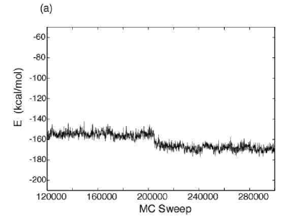
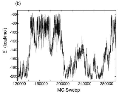
Figure 1: Time series (from 120,000 MC sweeps to 300,000 MC sweeps) of potential energy of the peptide fragment of ribonuclease T1 from (a) a conventional canonical MC simulation at $T=200$ K and (b) a multicanonical MC simulation.

We see that the canonical simulation thermalize very slowly. On the other hand, the MUCA simulation indeed performed a random walk in potential energy space covering a very wide energy range. Four conformations chosen during this period (from 120,000 MC sweeps to 300,000 MC sweeps) are shown in Figure 2 for the canonical simulation and in Figure 3 for the MUCA simulation. We see that the MUCA simulation samples much wider conformational space than the conventional canonical simulation.

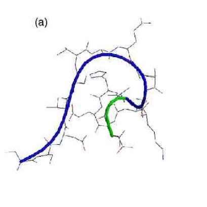
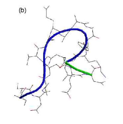
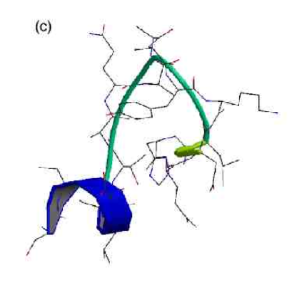
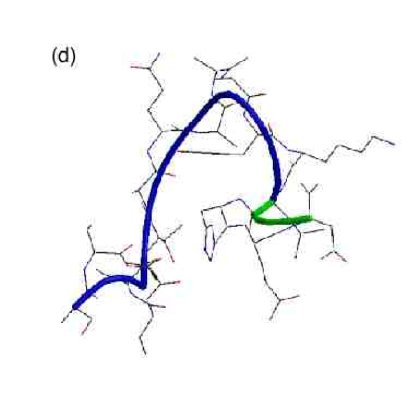
Figure 2: Typical snapshots from the canonical MC simulation of Figure 1(a). The figures were created with Molscript [121] and Raster3D [122, 123].

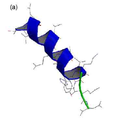
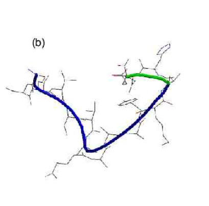
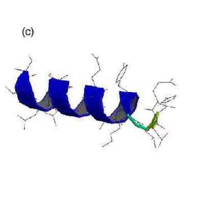
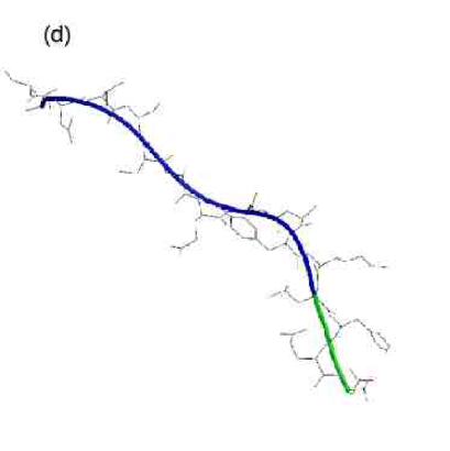
Figure 3: Typical snapshots from the multicanonical MC simulation of Figure 1(b). The figures were created with Molscript [121] and Raster3D [122, 123].

The next examples of the systems that we studied by multicanonical MC simulations are homo-oligomer systems. We studied the helix-forming tendencies of three amino-acid homo-oligomers of length 10 in gas phase [20, 21] and in aqueous solution (the solvent effects are represented by the term that is proportional to solvent-accessible surface area) [42]. Three characteristic amino acids, alanine (helix former), valine (helix indifferent), and glycine (helix breaker) were considered. In Figure 4 the lowest-energy conformations obtained both in gas phase and in aqueous solution by MUCA simulations are shown [42]. The lowest-energy conformations of (Ala)₁₀ (Figures 2(a) and 2(b)) have six intrachain backbone hydrogen bonds that characterize the $\alpha$-helix and are indeed completely helical. Those of (Val)₁₀ are also in almost ideal helix state (from residue 2 to residue 9 in gas phase and from residue 2 to residue 8 in aqueous solution). On the other hand, those of (Gly)₁₀ are not helical and rather round.

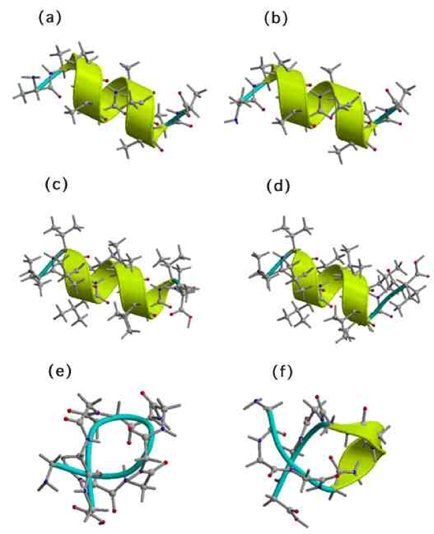
Figure 4: The lowest-energy conformations of (Ala)₁₀ ((a) and (b)), (Val)₁₀ ((c) and (d)), and (Gly)₁₀ ((e) and (f)) obtained from the multicanonical MC simulations in gas phase and in aqueous solution, respectively. The figures were created with Molscript [121] and Raster3D [122, 123].

We calculated the average values of the total potential energy and its component terms of (Ala)₁₀ as a function of temperature both in gas phase and in aqueous solution [42]. The results are shown in Figure 5. For homo-alanine in gas phase, all the conformational energy terms increase monotonically as temperature increases. The changes of each component terms are very small except for the Lennard-Jones term, $E_{\rm v}$, indicating that $E_{\rm v}$ plays an important role in the folding of homo-alanine [21].

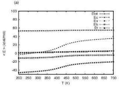
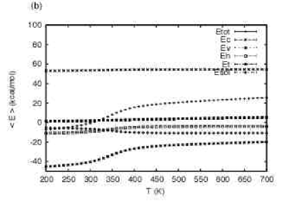
Figure 5: Average of the total potential energy $E_{\rm tot}$ and averages of its component terms, electrostatic energy $E_{\rm c}$, hydrogen-bond energy $E_{\rm h}$, Lennard-Jones energy $E_{\rm v}$, torsion energy $E_{\rm t}$, and solvation free energy $E_{\rm sol}$ (only for the case in aqueous solution) for homo-alanine as a function of temperature $T$ (a) in gas phase and (b) in aqueous solution. The values for each case were calculated from one multicanonical production run of 1,000,000 MC sweeps by the single-histogram reweighting techniques.

In aqueous solution the overall behaviors of the conformational energy terms are very similar to those in gas phase. The solvation term, on the other hand, decreases monotonically as temperature increases. These results imply that the solvation term favors random-coil conformations, while the conformational terms favor helical conformations.

The rapid changes (decrease for the solvation term and increase for the rest of the terms) of all the average values occur at the same temperature (around at 420 K in gas phase and 340 K in solvent). We thus calculated the specific heat for (Ala)₁₀ as a function of temperature. The specific heat here is defined by the following equation:

$$C(T)={\beta}^{2}\ \frac{<E_{\rm tot}^{2}>_{T}-{<E_{\rm tot}>_{T}}^{2}}{N},$$ (58)

where $N\ (=10)$ is the number of residues in the oligomer. In Figure 6 we show the results. We observe sharp peaks in the specific heat for both environment. The temperatures at the peak, helix-coil transition temperatures, are $T_{c}\approx$ 420 K and 340 K in gas phase and in aqueous solution, respectively.

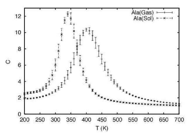
Figure 6: Specific heat $C$ as a function of temperature $T$ for (Ala)₁₀ in gas phase and in aqueous solution. The values for each case were calculated from one multicanonical production run of 1,000,000 MC sweeps by the single-histogram reweighting techniques.

We calculated the average number of helical residues $<n>_{T}$ in a conformation as a function of temperature. In Figure 7 we show the average helicity $<n>_{T}$ as a function of temperature for the three homo-oligomers in aqueous solution. The average helicity tends to decrease monotonically as the temperature increases because of the increased thermal fluctuations.

At $T=200$ K, $<n>_{T}$ for homo-alanine is 8. If we neglect the terminal residues, in which $\alpha$-helix tends to be frayed, $n=8$ corresponds to the maximal helicity, and the conformation can be considered completely helical. The homo-alanine is thus in an ideal helical structure at $T=200$ K. Around the room temperature, the homo-alanine is still substantially helical ($\approx 70$ % helicity). This is consistent with the experimental fact that alanine is a strong helix former. We observe that $<n>_{T}$ is 5 (50 % helicity) at the transition temperature obtained from the peak in specific heat (around 340 K). This implies that the peak in specific heat indeed implies a helix-coil transition between an ideal helix and a random coil.

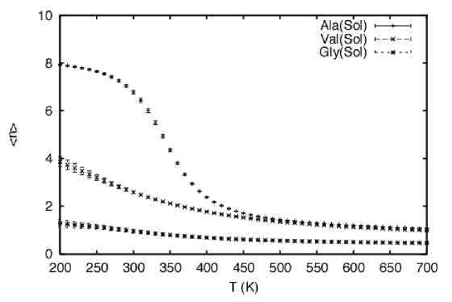
Figure 7: Average helicity $<n>_{T}$ as a function of temperature $T$ for (Ala)₁₀, (Val)₁₀, and (Gly)₁₀ in aqueous solution. The values for each case were calculated from one multicanonical production run of 1,000,000 MC sweeps by the single-histogram reweighting techniques.

The next example is a penta peptide, Met-enkephalin, whose amino-acid sequence is: Tyr-Gly-Gly-Phe-Met. Since this is one of the simplest peptides with biological functions, it served as a bench mark system for many simulations.

Here, we present the latest results of a multicanonical MC simulation of Met-enkephalin in gas phase [38]. The conformations were classified into six groups of similar structures according to their intra-chain hydrogen bonds. In Figure 8 we show the lowest-energy conformations in each group identified by the MUCA simulation. The lowest-energy conformation of group C25 (Figure 8(a)) has two hydrogen bonds, connecting residues 2 and 5, and forms a type II^′ $\beta$-turn. The ECEPP/2 energy of the conformation is $-12.2$ kcal/mol, and this conformation corresponds to the global-minimum-energy state of Met-enkephalin in gas phase. The lowest-energy conformation of group C14 (Figure 8(b)) has two hydrogen bonds, connecting residues 1 and 4, and forms a type II $\beta$-turn. The energy is $-$11.1 kcal/mol, and this conformation corresponds to the second-lowest-energy state. Other groups correspond to high-energy states.

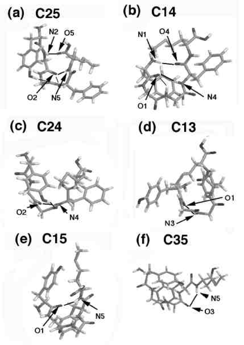
Figure 8: The lowest-energy conformations in each group obtained by the multicanonical MC simulation of 1,000,000 MC sweeps. The lowest-energy conformations correspond to groups (a) C25, (b) C14, (c) C24, (d) C13, (e) C15, and (f) C35. The figures were created with RasMol [124].

We now study the distributions of conformations in these groups as a function of temperature. The results are shown in Figure 9. As can be seen in the Figure, group C25 is dominant at low temperatures. Conformations of group C14 start to appear from $T\approx 100$ K. At $T\approx 300$ K, the distributions of these two groups, C25 and C14, balance ( $\approx$ 25 % each) and constitute the main groups. Above $T\approx 300$ K, the contributions of other groups become non-negligible (those of group C24 and group C13 are about 10 % and 8 %, respectively, at $T=400$ K). Note that the distribution of conformations that do not belong to any of the six groups monotonically increases as the temperature is raised. This is because random-coil conformations without any intrachain hydrogen bonds are favored at high temperatures.

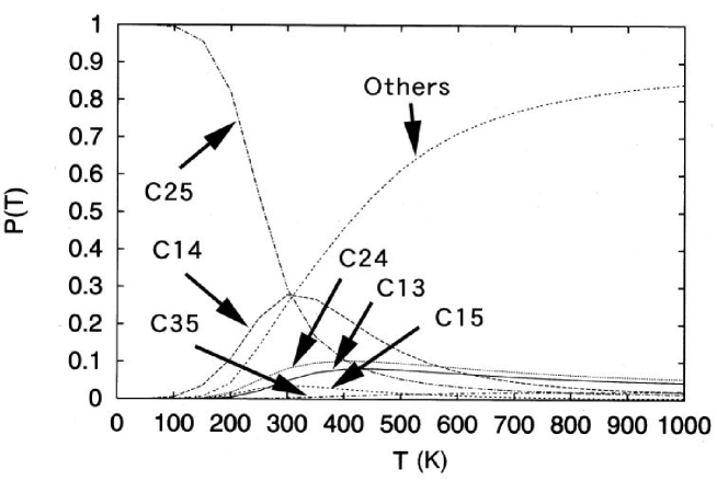
Figure 9: The distributions of each group of similar strucutres as a function of temperature.

The same peptide in gas phase was studied by the replica-exchange MD simulation [78]. We made an MD simulation of $2\times 10^{6}$ time steps (or, 1.0 ns) for each replica, starting from an extended conformation. We used the following eight temperatures: 700, 585, 489, 409, 342, 286, 239, and 200 K, which are distributed exponentially, following the annealing schedule of simulated annealing simulations [97]. As is shown below, this choice already gave an optimal temperature distribution. The replica exchange was tried every 10 fs, and the data were stored just before the replica exchange for later analyses.

As for expectation values of physical quantities at various temperatures, we used the multiple-histogram reweighting techniques of Eqs. (30) and (31). We remark that for biomolecular systems the integrated autocorrelation times, $\tau_{m}$, in the reweighting formulae (see Eq. (30)) can safely be set to be a constant [3], and we do so throughout the analyses in this section.

For an optimal performance of REM simulations the acceptance ratios of replica exchange should be sufficiently uniform and large (say, $>10$ %). In Table 1 we list these quantities. The values are indeed uniform (all about 15 % of acceptance probability) and large enough (more than 10 %).

Table 1: Acceptance Ratios of Replica Exchange Corresponding to Pairs of Neighboring Temperatures

Pair of Temperatures (K)	Acceptance Ratio
200 $\longleftrightarrow$ 239	0.160
239 $\longleftrightarrow$ 286	0.149
286 $\longleftrightarrow$ 342	0.143
342 $\longleftrightarrow$ 409	0.139
409 $\longleftrightarrow$ 489	0.142
489 $\longleftrightarrow$ 585	0.146
585 $\longleftrightarrow$ 700	0.146

The results in Table 1 imply that one should observe a free random walk in temperature space. The results for one of the replicas are shown in Figure 10(a). We do observe a random walk in temperature space between the lowest and highest temperatures. In Figure 10(b) the corresponding time series of the total potential energy is shown. We see that a random walk in potential energy space between low and high energies is realized. We remark that the potential energy here is that of AMBER in Ref. [110]. Note that there is a strong correlation between the behaviors in Figures 10(a) and 10(b).

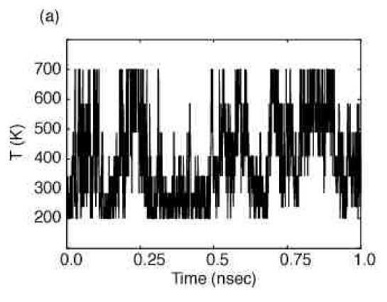
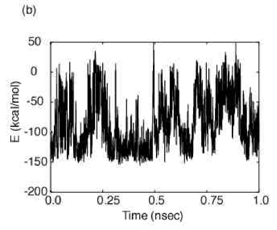
Figure 10: Time series of (a) temperature exchange and (b) the total potential energy for one of the replicas from a replica-exchange MD simulation of Met-enkephalin in gas phase.

In Figure 11 the canonical probability distributions obtained at the chosen eight temperatures from the replica-exchange simulation are shown. We see that there are enough overlaps between all pairs of distributions, indicating that there will be sufficient numbers of replica exchanges between pairs of replicas (see Table 1).

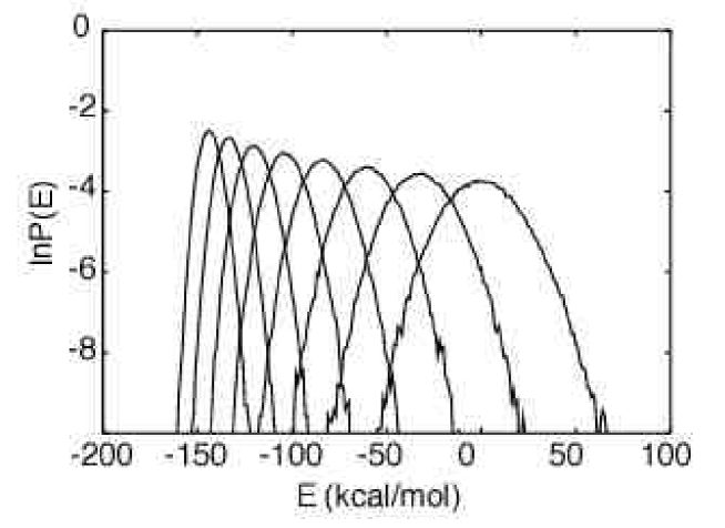
Figure 11: The canonical probability distributions of the total potential energy of Met-enkephalin in gas phase obtained from the replica-exchange MD simulation at the eight temperatures. The distributions correspond to the following temperatures (from left to right): 200, 239, 286, 342, 409, 489, 585, and 700 K.

We further compare the results of the replica-exchange simulation with those of a single canonical MD simulation (of 1 ns) at the corresponding temperatures. In Figure 12 we compare the distributions of a pair of dihedral angles $(\phi,\psi)$ of Gly-2 at two extreme temperatures ($T=200$ K and 700 K). While the results at $T=200$ K from the regular canonical simulation are localized with only one dominant peak, those from the replica-exchange simulation have several peaks (compare Figures 12(a) and 12(b)). Hence, the replica-exchange run samples much broader configurational space than the conventional canonical run at low temperatures. The results at $T=700$ K (Figures 12(c) and 12(d)), on the other hand, are similar, implying that a regular canonical simulation can give accurate thermodynamic quantities at high temperatures.

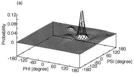
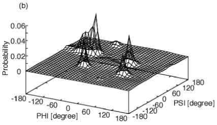
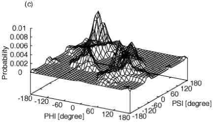
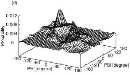
Figure 12: Distributions of a pair of dihedral angles $(\phi,\psi)$ of Gly-2 for: (a) $T=200$ K from a regular canonical MD simulation, (b) $T=200$ K from the replica-exchange MD simulation, (c) $T=700$ K from a regular canonical MD simulation, and (d) $T=700$ K from the replica-exchange MD simulation.

In Figure 13 we show the average total potential energy as a function of temperature. As expected from the results of Figure 12, we observe that the canonical simulations at low temperatures got trapped in states of energy local minima, resulting in the discrepancies in average values between the results from the canonical simulations and those from the replica-exchange simulation.

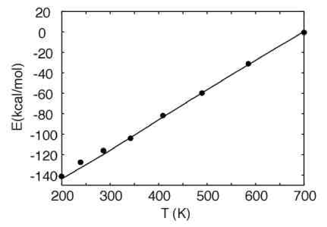
Figure 13: Average total potential energy of Met-enkephalin in gas phase as a function of temperature. The solid curve is the result from the replica-exchange MD simulation and the dots are those of regular canonical MD simulations.

We now present the results of MD simulations based on replica-exchange multicanonical algorithm and multicanonical replica-exchange method [90]. The Met-enkephalin in gas phase was studied again. The potential energy is, however, that of AMBER in Ref. [111] instead of Ref. [110]. In Table 2 we summarize the parameters of the simulations that were performed. As discussed in the previous section, REMUCA consists of two simulations: a short REM simulation (from which the density of states of the system, or the multicanonical weight factor, is determined) and a subsequent production run of MUCA simulation. The former simulation is referred to as REM1 and the latter as MUCA1 in Table 2. A production run of MUCAREM simulation is referred to as MUCAREM1 in Table 2, and it uses the same density of states that was obtained from REM1. Finally, a production run of the original REM simulation was also performed for comparison and it is referred to as REM2 in Table 2. The total simulation time for the three production runs (REM2, MUCA1, and MUCAREM1) was all set equal (i.e., 5 ns).

Table 2: Summary of Parameters in REM, REMUCA, and MUCAREM Simulations

Run	No. of Replicas, $M$	Temperature, $T_{m}$ (K) ($m=1,\cdots,M$)	MD Steps
REM1	10	200, 239, 286, 342, 409,	$2\times 10^{5}$
		489, 585, 700, 836, 1000
REM2	10	200, 239, 286, 342, 409,	$1\times 10^{6}$
		489, 585, 700, 836, 1000
MUCA1	1	1000	$1\times 10^{7}$
MUCAREM1	4	375, 525, 725, 1000	$2.5\times 10^{6}$

After the simulation of REM1 is finished, we obtained the density of states, $n(E)$, by the multiple-histogram reweighting techniques of Eqs. (30) and (31). The density of states will give the average values of the potential energy from Eq. (20), and we found

$$\left\{\begin{array}[]{rl}E_{1}&=~{}<E>_{T_{1}}=-30~{}{\rm kcal/mol}~{},\\ E_{M}&=~{}<E>_{T_{M}}=195~{}{\rm kcal/mol}~{}.\end{array}\right.$$ (59)

Then our estimate of the density of states is reliable in the range $E_{1}\leq E\leq E_{M}$. The multicanonical potential energy ${\cal E}_{mu}^{\{0\}}(E)$ was thus determined for the three energy regions ($E<E_{1}$, $E_{1}\leq E\leq E_{M}$, and $E>E_{M}$) from Eq. (49). Namely, the multicanonical potential energy, $E_{mu}(E;T_{0})$, in Eq. (9) and its derivative, $\frac{\partial E_{mu}(E;T_{0})}{\partial E}$, were determined by fitting $\ln n(E)$ by cubic spline functions in the energy region of ($-30\leq E\leq 195$ kcal/mol) [90]. Here, we have set the arbitrary reference temperature to be $T_{0}=1000$ K. Outside this energy region, $E_{mu}(E;T_{0})$ was linearly extrapolated as in Eq. (49).

After determining the multicanonical weight factor, we carried out a multicanonical MD simulation of $1\times 10^{7}$ steps (or 5 ns) for data collection (MUCA1 in Table 2). In Figure 14 the probability distribution obtained by MUCA1 is plotted. It can be seen that a good flat distribution is obtained in the energy region $E_{1}\leq E\leq E_{M}$. In Figure 14 the canonical probability distributions that were obtained by the reweighting techniques at $T=T_{1}=200$ K and $T=T_{M}=1000$ K are also shown (these results are essentially identical to one another among MUCA1, MUCAREM1, and REM2, as discussed below). Comparing these curves with those of MUCA1 in the energy regions $E<E_{1}$ and $E>E_{M}$ in Figure 14, we confirm our claim in the previous section that MUCA1 gives canonical distributions at $T=T_{1}$ for $E<E_{1}$ and at $T=T_{M}$ for $E>E_{M}$, whereas it gives a multicanonical distribution for $E_{1}\leq E\leq E_{M}$.

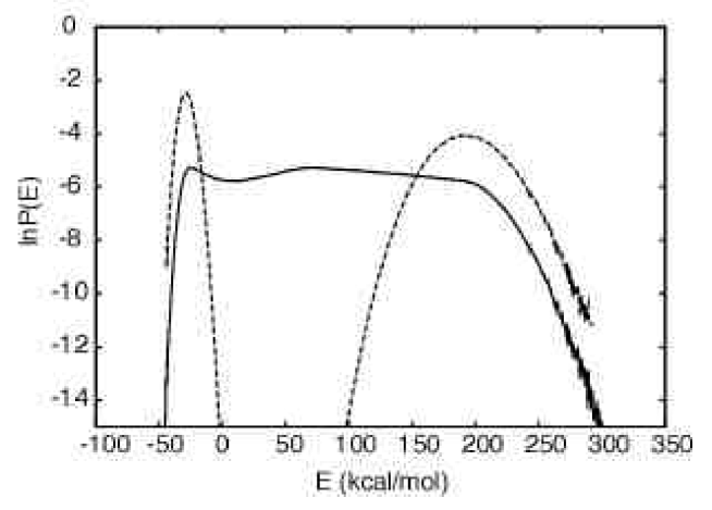
Figure 14: Probability distribution of potential energy of Met-enkephalin in gas phase that was obtained from MUCA1 (see Table 2). The dotted curves are the probability distributions of the reweighted canonical ensemble at $T=200$ K (left) and 1000 K (right).

In the previous works of multicanonical simulations of Met-enkephalin in gas phase (see, for instance, Refs. [14, 38]), at least several iterations of trial simulations were required for the multicanonical weight determination. We emphasize that in the present case of REMUCA (REM1), only one simulation was necessary to determine the optimal multicanonical weight factor that can cover the energy region corresponding to temperatures between 200 K and 1000 K.

From the density of states obtained by REMUCA (i.e., REM1), we prepared the multicanonical weight factors (or the multicanonical potential energies) for the MUCAREM simulation (see Eq. (53)). The parameters of MUCAREM1, such as energy bounds $E_{L}^{\{m\}}$ and $E_{H}^{\{m\}}$ ($m=1,\cdots,{\cal M}$) are listed in Table 3. The choices of $T_{L}^{\{m\}}$ and $T_{H}^{\{m\}}$ are, in general, arbitrary, but significant overlaps between the probability distributions of adjacent replicas are necessary. The replica-exchange process in MUCAREM1 was tried every 200 time steps (or 100 fs). It is less frequent than in REM1 (or REM2). This is because we wanted to ensure a sufficient time for system relaxation.

Table 3: Summary of Parameters in MUCAREM1

$m$	$T_{L}^{\{m\}}$ (K)	$T_{H}^{\{m\}}$ (K)	$T_{m}$ (K)	$E_{L}^{\{m\}}$ (kcal/mol)	$E_{H}^{\{m\}}$ (kcal/mol)
1	200	375	375	$-30$	20
2	300	525	525	$-5$	65
3	375	725	725	20	120
4	525	1000	1000	65	195

In Figure 15 the probability distributions of potential energy obtained by MUCAREM1 are shown. As expected, we observe that the probability distributions corresponding to the temperature $T_{m}$ are essentially flat for the energy region $E_{L}^{\{m\}}\leq E\leq E_{H}^{\{m\}}$, are of the canonical simulation at $T=T_{L}^{\{m\}}$ for $E<E_{L}^{\{m\}}$, and are of the canonical simulation at $T=T_{H}^{\{m\}}$ for $E>E_{H}^{\{m\}}$ ($m=1,\cdots,{\cal M}$). As a result, each distribution in MUCAREM is much broader than those in the conventional REM and a much smaller number of replicas are required in MUCAREM than in REM (${\cal M}=4$ in MUCAREM versus $M=10$ in REM).

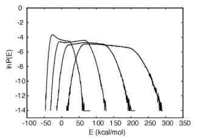
Figure 15: Probability distributions of potential energy obtained from MUCAREM1 (see Tables 2 and 3).

In Figure 16 the time series of potential energy for the first 500 ps of REM2 (a), MUCA1 (b), and MUCAREM1 (c) are plotted. They all exhibit a random walk in potential energy space, implying that they all perfomed properly as generalized-ensemble algorithms. To check the validity of the canonical-ensemble expectation values calculated by the new algorithms, we compare the average potential energy as a function of temperature in Figure 17. In REM2 and MUCAREM1 we used the multiple-histogram techniques [2, 3], whereas the single-histogram method [1] was used in MUCA1. We can see a perfect coincidence of these quantities among REM2, MUCA1, and MUCAREM1 in Figure 17.

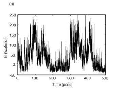
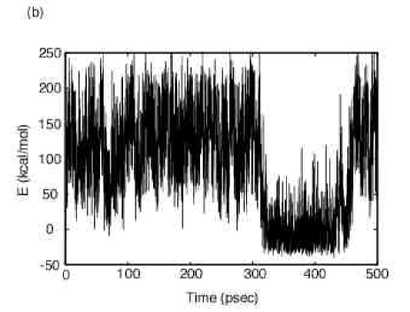
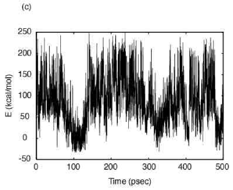
Figure 16: Time series of potential energy of Met-enkephalin in gas phase for one of the replicas in (a) REM2, (b) MUCA1, and (c) MUCAREM1 (see Tables 2 and 3 for the parameters of the simulations).

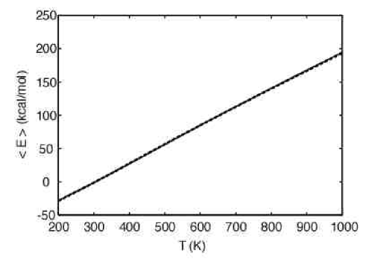
Figure 17: The average potential energy of Met-enkephalin in gas phase as a function of temperature. The solid, dotted, and dashed curves are obtained from REM2, MUCA1, and MUCAREM1, respectively (see Tables 2 and 3 for the parameters of the simulations).

We now present the results of a replica-exchange simulated tempering MC simulation of Met-enkephalin in gas phase [91]. The potential energy is again that of ECEPP/2 [93]–[95]. In Table 4 we summarize the parameters of the simulations that were performed. As described in the previous section, REST consists of two simulations: a short REM simulation (from which the dimensionless Helmholtz free energy, or the simulated tempering weight factor, is determined) and a subsequent ST production run. The former simulation is referred to as REM1 and the latter as ST1 in Table 4. In REM1 there exist 8 replicas with 8 different temperatures ($M=8$), ranging from 50 K to 1000 K as listed in Table 4 (i.e., $T_{1}=50$ K and $T_{M}=T_{8}=1000$ K). The same set of temperatures were also used in ST1. The temperatures were distributed exponentially between $T_{1}$ and $T_{M}$, following the optimal distribution found in the previous simulated annealing schedule [97], simulated tempering run [51], and replica-exchange simulation [78]. After estimating the weight factor, we made a ST production run of $10^{6}$ MC sweeps (ST1). In REM1 and ST1, a replica exchange and a temperature update, respectively, were tried every 10 MC sweeps.

Table 4: Summary of Parameters in REST Simulations

Run	No. of Replicas, $M$	Temperature, $T_{m}$ (K) ($m=1,\cdots,M$)	MC Sweeps
REM1	8	50, 77, 118, 181, 277, 425, 652, 1000	$5\times 10^{4}$
ST1	1	50, 77, 118, 181, 277, 425, 652, 1000	$1\times 10^{6}$

We first check whether the replica-exchange simulation of REM1 indeed performed properly. For an optimal performance of REM the acceptance ratios of replica exchange should be sufficiently uniform and large (say, $>10$ %). In Table 5 we list these quantities. It is clear that both points are met in the sense that they are of the same order (the values vary between 10 % and 40 %).

Table 5: Acceptance Ratios of Replica Exchange in REM1 of Table 4

Pair of Temperatures (K)	Acceptance Ratio
50   $\longleftrightarrow$   77	0.30
77   $\longleftrightarrow$   118	0.27
118   $\longleftrightarrow$   181	0.22
181   $\longleftrightarrow$   277	0.17
277   $\longleftrightarrow$   425	0.10
425   $\longleftrightarrow$   652	0.27
652   $\longleftrightarrow$   1000	0.40

After determining the simulated tempering weight factor, we carried out a long ST simulation for data collection (ST1 in Table 4). In Figure 18 the time series of temperature and potential energy from ST1 are plotted. In Figure 18(a) we observe a random walk in temperature space between the lowest and highest temperatures. In Figure 18(b) the corresponding random walk of the total potential energy between low and high energies is observed. Note that there is a strong correlation between the behaviors in Figures 18(a) and 18(b), as there should. It is known from our previous works that the global-minimum-energy conformation for Met-enkephalin in gas phase has the ECEPP/2 energy value of $-12.2$ kcal/mol [18, 38]. Hence, the random walk in Figure 12(b) indeed visited the global-minimum region many times. It also visited high energy regions, judging from the fact that the average potential energy is around 15 kcal/mol at $T=1000$ K [14, 38] (see also Figure 19 below).

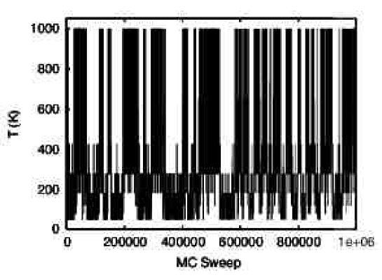
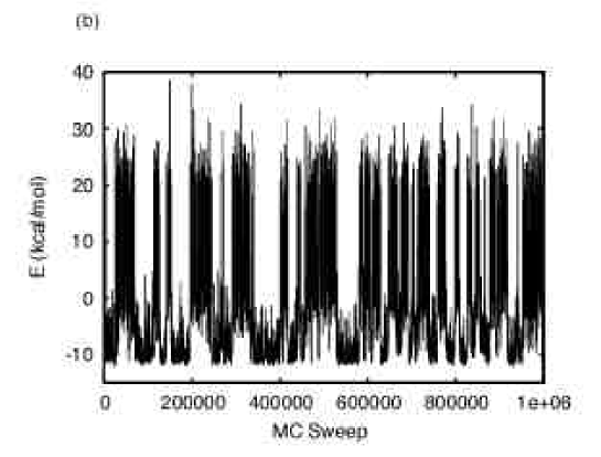
Figure 18: Time series of (a) temperature and (b) potential energy in ST1 (see Table 4 for the parameters of the simulation).

For an optimal performance of ST, the acceptance ratios of temperature update should be sufficiently uniform and large. In Table 6 we list these quantities. It is clear that both points are met (the values vary between 26 % and 57 %); we find that the present ST run (ST1) indeed properly performed. We remark that the acceptance ratios in Table 6 are significantly larger and more uniform than those in Table 5, suggesting that ST runs can sample the configurational space more effectively than REM runs, provided the optimal weight factor is obtained.

Table 6: Acceptance Ratios of Temperature Update in ST1

Pair of Temperatures (K)	Acceptance Ratio
50   $\longrightarrow$   77	0.47
77   $\longrightarrow$   50	0.47
77   $\longrightarrow$   118	0.43
118   $\longrightarrow$   77	0.43
118   $\longrightarrow$   181	0.37
181   $\longrightarrow$   118	0.42
181   $\longrightarrow$   277	0.29
277   $\longrightarrow$   181	0.29
277   $\longrightarrow$   425	0.30
425   $\longrightarrow$   277	0.26
425   $\longrightarrow$   652	0.43
652   $\longrightarrow$   425	0.42
652   $\longrightarrow$   1000	0.57
1000   $\longrightarrow$   652	0.56

We remark that the details of Monte Carlo versions of REMUCA and MUCAREM have also been worked out and tested with Met-enkephalin in gas phase [125]. Here in Figure 19, we just show the average ECEPP/2 potential energy as a function of temperature that was calculated from the four generalized-ensemble algorithms, MUCA, REMUCA, MUCAREM, and REST [125]. The results are in good agreement.

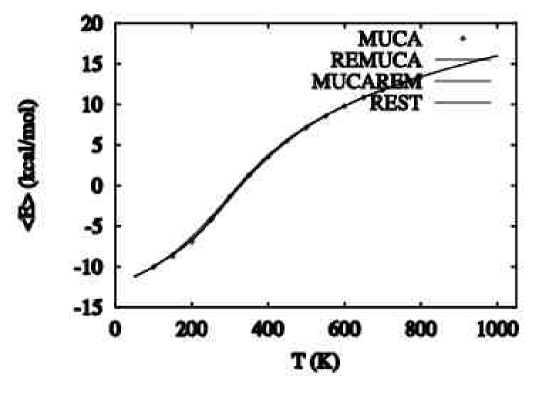
Figure 19: The average potential energy of Met-enkephalin in gas phase as a function of temperature. The results from the four generalized-ensemble algorithms, MUCA, REMUCA, MUCAREM, and REST, are superimposed.

We have so far presented the results of generalized-ensemble simulations of Met-enkephalin in gas phase. However, peptides and proteins are usually in aqueous solution. We therefore want to incorporate rigorous solvation effects in our simulations in order to compare with experiments.

Our first example with rigorous solvent effects is a multicanonical MC simulation, where the solvation term was included by the RISM theory [44]. While low-energy conformations of Met-enkephalin in gas phase are compact and form $\beta$-turn structures [38], it turned out that those in aqueous solution are extended. In Figure 20 we show the lowest-energy conformations of Met-enkephalin obtained during the multicanonical MC simulation with RISM theory incorporated [44]. They exhibit characteristics of almost fully extended backbone structure with large side-chain fluctuations. The results are in accord with the observations in NMR experiments, which also suggest extended conformations [126].

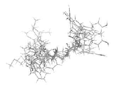
Figure 20: Superposition of eight representative low-energy conformations of Met-enkephalin obtained by the multicanonical MC simulation in aqueous solution based on RISM. The figure was created with RasMol [124].

We also calculated an average of the end-to-end distance of Met-enkephalin as a function of temperature. The results in aqueous solution (the present simulation) and in the gas phase (a previous simulation [38]) are compared in Figure 21. The end-to-end distance in aqueous solution at all temperatures varies little (around 12 Å); the conformations are extended in the entire temperature range. On the other hand, in the gas phase, the end-to-end distance is small at low temperatures due to intrachain hydrogen bonds, while the distance is large at high temperatures, because these intrachain hydrogen bonds are broken.

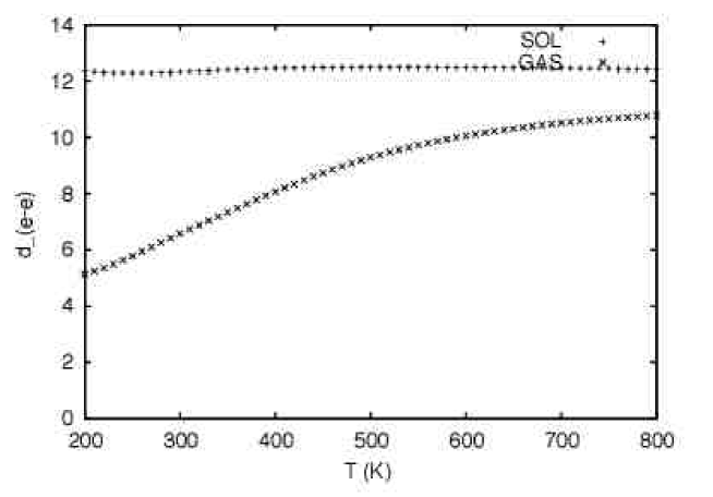
Figure 21: Average end-to-end distance of Met-enkephalin in aqueous solution (SOL) and in gas phase (GAS) as a function of temperature. Here, the end-to-end distance is defined as the distance between the nitrogen atom at the N terminus and the oxygen atom at the C terminus.

The same peptide was also studied by MD simulations of replica-exchange and other generalized-ensemble simulations in aqueous solution based on TIP3P water model [127]. Two AMBER force fields [111, 112] were used. The number of water molecules was 526 and they were placed in a sphere of radius of 16 Å. The initial configuration is shown in Figure 22.

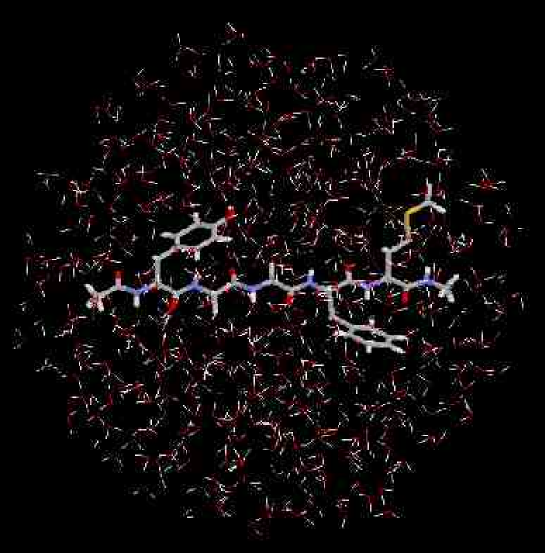
Figure 22: Initial configuration of replica-exchange MD simulations of Met-enkephalin in aqueous solution with 526 TIP3P water molecules.

In Figure 23 the canonical probability distributions obtained at the 24 temperatures from the replica-exchange simulation are shown. We see that there are enough overlaps between all pairs of distributions, indicating that there will be sufficient numbers of replica exchanges between pairs of replicas. The corresponding time series of the total potential energy for one of the replicas is shown in Figure 24. We do observe a random walk in potential energy space, which covers an energy range of as much as 2,000 kcal/mol.

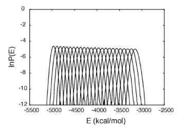
Figure 23: The canonical probability distributions of the total potential energy of Met-enkephalin in aqueous solution obtained from the replica-exchange MD simulation at the 24 temperatures.

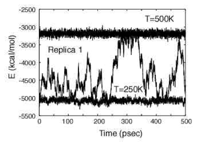
Figure 24: Time series of the total potential energy of Met-enkephalin in aqueous solution obtained for one of the replicas from the replica-exchange MD simulation. Corresponding times series in the canonical ensemble at temperatures 250 K and 500 K are also shown.

Finally, the average end-to-end distance as a function of temperature was calculated by the multiple-histogram reweighting techniques of Eqs. (30) and (31). The results both in gas phase and in aqueous solution are shown in Figure 25. The results are in good agreement with those of ECEPP/2 energy plus RISM solvation theory [44] in the sense that Met-enkephalin is compact at low temperatures and extended at high temperatures in gas phase and extended in the entire temperature range in aqueous solution (compare Figures 21 and 25).

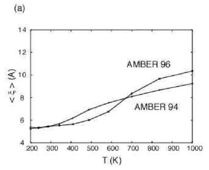
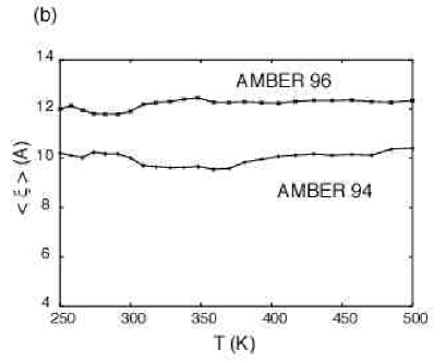
Figure 25: Average end-to-end distance of Met-enkephalin (a) in gas phase and (b) in aqueous solution as a function of temperature.

4 CONCLUSIONS

In this article we have reviewed uses of generalized-ensemble algorithms in molecular simulations of biomolecules. A simulation in generalized ensemble realizes a random walk in potential energy space, alleviating the multiple-minima problem that is a common difficulty in simulations of complex systems with many degrees of freedom.

Detailed formulations of the three well-known generalized-ensemble algorithms, namely, multicaonical algorithm (MUCA), simulated tempering (ST), and replica-exchange method (REM), were given. We then introduced three new generalized-ensemble algorithms that combine the merits of the above three methods, which we refer to as replica-exchange multicanonical algorithm (REMUCA), replica-exchange simulated tempering (REST), and multicanonical replica-exchange method (MUCAREM).

With these new methods available, we believe that we now have working simulation algorithms which we can use for conformational predictions of peptides and proteins from the first principles, using the information of their amino-acid sequence only. It is now high time that we addressed the question of the validity of the standard potential energy functions such as AMBER, CHARMM, GROMOS, ECEPP, etc. For this purpose, conventional simulations in the canonical ensemble are of little use because they will necessarily get trapped in states of local-minmum-energy states. It is therefore essential to use generalized-ensemble algorithms in order to test and develop accurate potential energy functions for biomolecular systems. Some preliminary results of comparisons of different versions of AMBER force fields were given in the present article. We remark that more detailed analyses that compare different versions of AMBER by multicanonical MD simulations already exist [128]. Likewise, the validity of solvation theories should also be tested. For this, RISM theory [105]–[107] can be very useful. For instance, we have successfully given a molecular mechanism of secondary structural transitions in peptides due to addition of alcohol to solvent [129], which is very difficult to attain by regular molecular simulations.

Acknowledgements:
Our simulations were performed on the Hitachi and other computers at the Research Center for Computational Science, Okazaki National Research Institutes. This work is supported, in part, by a grant from the Research for the Future Program of the Japan Society for the Promotion of Science (JSPS-RFTF98P01101).

References

- [1] Ferrenberg, A.M. & Swendsen, R.H. (1988) Phys. Rev. Lett. 61, 2635–2638; ibid. (1989) 63, 1658.
- [2] Ferrenberg, A.M. & Swendsen, R.H. (1989) Phys. Rev. Lett. 63, 1195–1198.
- [3] Kumar, S., Bouzida, D., Swendsen, R.H., Kollman, P.A. & Rosenberg, J.M. (1992) J. Comput. Chem. 13, 1011–1021.
- [4] Berg, B.A. & Neuhaus, T. (1991) Phys. Lett. B267, 249–253.
- [5] Berg, B.A. & Neuhaus, T. (1992) Phys. Rev. Lett. 68, 9–12.
- [6] Berg, B.A. (2000) Fields Institute Communications 26, 1–24; also see cond-mat/9909236.
- [7] Lee, J. (1993) Phys. Rev. Lett. 71, 211–214; ibid. 71, 2353.
- [8] Bartels, C. & M. Karplus, M. (1998) J. Phys. Chem. B 102, 865–880.
- [9] Berg, B.A., Hansmann, U.H.E. & Okamoto, Y. (1995) J. Phys. Chem. 99, 2236–2237.
- [10] Berg, B.A. & Celik, T. (1992) Phys. Rev. Lett. 69, 2292–2295.
- [11] Berg, B.A., Celik, T. & Hansmann, U.H.E. (1993) Europhys. Lett. 22, 63–68.
- [12] Berg, B.A. & Janke, W. (1998) Phys. Rev. Lett. 80, 4771–4774.
- [13] Hatano, N. & Gubernatis, J.E. (2000) Prog. Theor. Phys. (Suppl.) 138, 442–447.
- [14] Hansmann, U.H.E. & Okamoto, Y. (1993) J. Comput. Chem. 14, 1333–1338.
- [15] Okamoto, Y. (1998) Recent Res. Devel. in Pure & Applied Chem. 2, 1–23.
- [16] Hansmann, U.H.E. & Okamoto, Y. (1999) in Annual Reviews of Computational Physics VI, Stauffer, D., Ed., World Scientific, Singapore, pp. 129–157.
- [17] Hansmann, U.H.E. & Okamoto, Y. (1999) Curr. Opin. Struct. Biol. 9, 177–183.
- [18] Hansmann, U.H.E. & Okamoto, Y. (1994) Physica A212, 415–437.
- [19] Hao, M.H. & Scheraga, H.A. (1994) J. Phys. Chem. 98, 4940–4948.
- [20] Okamoto, Y., Hansmann, U.H.E. & Nakazawa, T. (1995) Chem. Lett. 1995, 391–392.
- [21] Okamoto, Y. & Hansmann, U.H.E. (1995) J. Phys. Chem. 99, 11276–11287.
- [22] Kidera, A. (1995) Proc. Natl. Acad. Sci. U.S.A. 92, 9886–9889.
- [23] Kolinski, A., Galazka, W. & Skolnick, J. (1996) Proteins 26, 271–287.
- [24] Urakami, N. & Takasu, M. (1996) J. Phys. Soc. Jpn. 65, 2694–2699.
- [25] Kumar, S., Payne, P. & Vásquez, M. (1996) J. Comput. Chem. 17, 1269–1275.
- [26] Hansmann, U.H.E., Okamoto, Y. & Eisenmenger, F. (1996) Chem. Phys. Lett. 259, 321–330.
- [27] Nakajima, N., Nakamura, H. & Kidera, A. (1997) J. Phys. Chem. B 101, 817–824.
- [28] Eisenmenger, F. & Hansmann, U.H.E. (1997) J. Phys. Chem. B 101, 3304–3310.
- [29] Higo, J., Nakajima, N., Shirai, H., Kidera, A. & Nakamura, H. (1997) J. Comput. Chem. 18, 2086–2092.
- [30] Nakajima, N., Higo, Kidera, A. & Nakamura, H. (1997) J. Chem. Phys. 278, 297–301.
- [31] Noguchi, H. & Yoshikawa, K. (1997) Chem. Phys. Lett. 278, 184–188.
- [32] Kolinski, A., Galazka, W. & Skolnick, J. (1998) J. Chem. Phys. 108, 2608–2617.
- [33] Iba, Y., Chikenji, G. & Kikuchi, M. (1998) J. Phys. Soc. Jpn. 67, 3327–3330.
- [34] Nakajima, N. (1998) Chem. Phys. Lett. 288, 319–326.
- [35] Hao, M.H. & Scheraga, H.A. (1998) J. Mol. Biol. 277, 973–983.
- [36] Shirai, H., Nakajima, N., Higo, J., Kidera, A. & Nakamura, H. (1998) J. Mol. Biol. 278, 481–496.
- [37] Schaefer, M., Bartels, C. & Karplus, M. (1998) J. Mol. Biol. 284, 835–848.
- [38] Mitsutake, A., Hansmann, U.H.E. & Okamoto, Y. (1998) J. Mol. Graphics Mod. 16, 226–238; 262–263.
- [39] Hansmann, U.H.E. & Okamoto, Y. (1999) J. Phys. Chem. B 103, 1595–1604.
- [40] Shimizu, H., Uehara, K., Yamamoto, K. & Hiwatari, Y. (1999) Mol. Sim. 22, 285–301.
- [41] Ono, S., Nakajima, N., Higo, J. & Nakamura, H. (1999) Chem. Phys. Lett. 312, 247–254.
- [42] Mitsutake, A. & Okamoto, Y. (2000) J. Chem. Phys. 112, 10638–10647.
- [43] Yasar, F., Celik, T., Berg, B.A. & Meirovitch, H. (2000) J. Comput. Chem. 21, 1251–1261.
- [44] Mitsutake, A., Kinoshita, M., Okamoto, Y. & Hirata, F. (2000) Chem. Phys. Lett. 329, 295–303.
- [45] Munakata, T. & Oyama, S. (1996) Phys. Rev. E 54, 4394–4398.
- [46] Lyubartsev, A.P., Martinovski, A.A., Shevkunov, S.V. & Vorontsov-Velyaminov, P.N. (1992) J. Chem. Phys. 96, 1776–1783.
- [47] Marinari E. & Parisi, G. (1992) Europhys. Lett. 19, 451–458.
- [48] Marinari, E., Parisi, G. & Ruiz-Lorenzo, J.J. (1998) in Spin Glasses and Random Fields, Young, A.P., Ed., World Scientific, Singapore, pp. 59–98.
- [49] Irbäck, A. & Potthast, F. (1995) J. Chem. Phys. 103, 10298–10305.
- [50] Hansmann, U.H.E. & Okamoto, Y. (1996) Phys. Rev. E 54, 5863–5865.
- [51] Hansmann, U.H.E. & Okamoto, Y. (1997) J. Comput. Chem. 18, 920–933.
- [52] Irbäck, A. & Sandelin, E. (1999) J. Chem. Phys. 110, 12256–12262.
- [53] Hesselbo, B. & Stinchcombe, R.B. (1995) Phys. Rev. Lett. 74, 2151–2155.
- [54] Smith, G.R. & Bruce, A.D. (1996) Phys. Rev. E 53, 6530–6543.
- [55] Hansmann, U.H.E. (1997) Phys. Rev. E 56, 6201–6203.
- [56] Berg, B.A. (1998) Nucl. Phys. B (Proc. Suppl.) 63A-C, 982–984.
- [57] Tsallis, C. (1988) J. Stat. Phys. 52, 479–487.
- [58] Hansmann, U.H.E. & Okamoto, Y. (1997) Phys. Rev. E 56, 2228–2233.
- [59] Hansmann, U.H.E., Eisenmenger, F. & Okamoto, Y. (1998) Chem. Phys. Lett. 297, 374–382.
- [60] Hansmann, U.H.E., Masuya, M. & Okamoto, Y. (1997) Proc. Natl. Acad. Sci. U.S.A. 94, 10652–10656.
- [61] Hansmann, U.H.E., Okamoto, Y. & Onuchic, J.N. (1999) Proteins 34, 472–483.
- [62] Andricioaei, I. & Straub, J.E. (1997) J. Chem. Phys. 107, 9117–9124.
- [63] Munakata, T. & Mitsuoka, S. (2000) J. Phys. Soc. Jpn. 69, 92–96.
- [64] Kirkpatrick, S., Gelatt, C.D. Jr. & Vecchi, M.P. (1983) Science 220, 671–680.
- [65] Tsallis, C. & Stariolo, D.A. (1996) Physica A233, 395–406.
- [66] Andricioaei, I. & Straub, J.E. (1996) Phys. Rev. E 53, R3055–R3058.
- [67] Hansmann, U.H.E. (1998) Physica A 242, 250–257.
- [68] Berne, B.J. & Straub, J.E. (1997) Curr. Opin. Struct. Biol. 7, 181–189.
- [69] Straub, J.E. & Andricioaei, I. (1999) Braz. J. Phys. 29, 179–186.
- [70] Hansmann, U.H.E. & Okamoto, Y. (1999) Braz. J. Phys. 29, 187–198.
- [71] Hukushima, K. & Nemoto, K. (1996) J. Phys. Soc. Jpn. 65, 1604–1608.
- [72] Hukushima, K., Takayama, H. & Nemoto, K. (1996) Int. J. Mod. Phys. C 7, 337–344.
- [73] Geyer, C.J. (1991) in Computing Science and Statistics: Proc. 23rd Symp. on the Interface, Keramidas, E.M., Ed., Interface Foundation, Fairfax Station, pp. 156–163.
- [74] Swendsen, R.H. & Wang, J.-S. (1986) Phys. Rev. Lett. 57, 2607–2609.
- [75] Tesi, M.C., van Rensburg, E.J.J., Orlandini, E. & Whittington, S.G. (1996) J. Stat. Phys. 82, 155–181.
- [76] Hansmann, U.H.E. (1997) Chem. Phys. Lett. 281, 140–150.
- [77] Falcioni, M. & Deem, M.W. (1999) J. Chem. Phys. 111, 6625–6632.
- [78] Sugita, Y. & Okamoto, Y. (1999) Chem. Phys. Lett. 314, 141–151.
- [79] Gront, D., Kolinski, A. & Skolnick, J. (2000) J. Chem. Phys. 113, 5065–5071.
- [80] Sugita, Y., Kitao, A. & Okamoto, Y. (2000) J. Chem. Phys. 113, 6042–6051.
- [81] Garcia, A.E. & Sanbonmatsu, K.Y. (2000) “Exploring the energy landscape of a hairpin in explicit solvent,” Proteins, in press.
- [82] Yan, Q. & de Pablo, J.J. (1999) J. Chem. Phys. 111, 9509–9516.
- [83] Nishikawa, Y., Ohtsuka, H., Sugita, Y., Mikami, M. & Okamoto, Y. (2000) Prog. Theor. Phys. (Suppl.) 138, 270–271.
- [84] Calvo, F., Neirotti, J.P., Freeman, D.L. & Doll, J.D. (2000) J. Chem. Phys. 112, 10350–10357.
- [85] Okabe, T., Kawata, M., Okamoto, Y. & Mikami, M. (2000) “Replica-exchange Monte Carlo method for the isobaric-isothermal ensemble,” submitted for publication.
- [86] Ishikawa, Y., Sugita, Y., Nishikawa, T. & Okamoto, Y. (2000) “Ab initio replica-exchange Monte Carlo method for cluster studies,” Chem. Phys. Lett., in press.
- [87] Yamamoto, R. & Kob, W. (2000) Phys. Rev. E 61, 5473–5476.
- [88] Hukushima, K. (1999) Phys. Rev. E 60, 3606–3614.
- [89] Bunker, A. & Dünweg, B. (2000) “Parallel excluded volume tempering for polymer melts,” Phys. Rev. E, in press.
- [90] Sugita, Y. & Okamoto, Y. (2000) Chem. Phys. Lett. 329, 261–270.
- [91] Mitsutake, A., & Okamoto, Y. (2000) Chem. Phys. Lett. 332, 131–138.
- [92] Metropolis, N., Rosenbluth, A.W., Rosenbluth, M.N., Teller, A.H. & Teller, E. (1953) J. Chem. Phys. 21, 1087–1092.
- [93] Momany, F.A., McGuire, R.F., Burgess, A.W. & Scheraga, H.A. (1975) J. Phys. Chem. 79, 2361–2381.
- [94] Némethy, G., Pottle, M.S. & Scheraga, H.A. (1983) J. Phys. Chem. 87, 1883–1887.
- [95] Sippl, M.J., Némethy, G. & Scheraga, H.A. (1984) J. Phys. Chem. 88, 6231–6233.
- [96] Kawai, H., Okamoto, Y., Fukugita, M., Nakazawa, T. & Kikuchi, T. (1991) Chem. Lett. 1991, 213–216.
- [97] Okamoto, Y., Fukugita, M., Nakazawa, T. & Kawai, H. (1991) Protein Eng. 4, 639–647.
- [98] Hingerty, B.E., Ritchie, R.H., Ferrell, T. & Turner, J.E. (1985) Biopolymers 24, 427–439.
- [99] Ramstein, J. & Lavery, R. (1988) Proc. Natl. Acad. Sci. U.S.A. 85, 7231–7235.
- [100] Okamoto, Y. (1994) Biopolymers 34, 529–539.
- [101] Daggett, V., Kollman, P.A. & Kuntz, I.D. (1991) Biopolymers 31, 285–304.
- [102] Ooi, T., Oobatake, M., Némethy, G. & Scheraga, H.A. (1987) Proc. Natl. Acad. Sci. U.S.A. 84, 3086–3090.
- [103] Masuya, M., in preparation.
- [104] Eisenhaber, F., Lijnzaad, P., Argos, P., Sander, C. & Scharf, M. (1995) J. Comput. Chem. 16, 273–284.
- [105] Chandler, D. & Andersen, H.C. (1972) J. Chem. Phys. 57, 1930–1937.
- [106] Hirata, F. & Rossky, P.J. (1981) Chem. Phys. Lett. 83, 329–334.
- [107] Perkyns, J.S. & Pettitt, B.M. (1992) J. Chem. Phys. 97, 7656–7666.
- [108] Berendsen, H.J.C., Grigera, J.R. & Straatsma, T.P. (1987) J. Phys. Chem. 91, 6269–6271.
- [109] Kinoshita, M., Okamoto, Y. & Hirata, F. (1997) J. Comput. Chem. 18, 1320–1326.
- [110] Weiner, S.J., Kollman, P.A., Nguyen, D.T. & Case, D.A. (1986) J. Comput. Chem. 7, 230–252.
- [111] Cornell, W.D., Cieplak, P., Bayly, C.I., Gould, I.R., Merz, K.M. Jr., Ferguson, D.M., Splellmeyer, D.C., Fox, T., Caldwell, J.W. & Kollman, P.A. (1995) J. Am. Chem. Soc. 117, 5179–5197.
- [112] Kollman, P., Dixon, R., Cornell, W., Fox, T. Chipot, C. & Pohorille, A. (1997) in Computer Simulation of Biomolecular Systems Vol. 3, van Gunsteren, W.F., Weiner, P.K. & Wilkinson, A.J., Eds., KLUWER/ESCOM, Dordrecht, pp. 83–96.
- [113] Sugita Y. & Kitao, A. (1998) Proteins 30, 388–400.
- [114] Kitao, A., Hayward, S. & Gō, N. (1998) Proteins 33, 496–517.
- [115] Morikami, K., Nakai, T., Kidera, A., Saito, M. & Nakamura, H. (1992) Comput. Chem. 16, 243–248.
- [116] Hoover, W.G., Ladd, A.J.C. & Moran, B. (1982) Phys. Rev. Lett. 48, 1818–1820.
- [117] Evans, D.J. & Morris, G.P. (1983) Phys. Lett. A98, 433–436.
- [118] Jorgensen, W.L., Chandreskhar, J., Madura, J.D., Impey, R.W. & Klein, M.L. (1982) J. Chem. Phys. 79, 926–935.
- [119] Myers, J.K., Pace, C.N. & Scholtz, J.M. (1997) Proc. Natl. Acad. Sci. U.S.A. 94, 2833–2837.
- [120] Mitsutake, A. & Okamoto, Y. (2000), in preparation.
- [121] Kraulis, P. J. (1991) J. Appl. Cryst. 24, 946–950.
- [122] Bacon, D. & Anderson, W. F. (1988) J. Mol. Graphics, 6, 219–220.
- [123] Merritt, E. A. & Murphy, M. E. P. (1994) Acta Cryst. D50, 869–873.
- [124] Sayle, R.A. & Milner-White, E.J. (1995) Trends Biochem. Sci. 20, 374–376.
- [125] Mitsutake, A., Sugita, Y. & Okamoto, Y. (2000), in preparation.
- [126] Graham, W.H., Carter, S.E. II & Hickes, P.R. (1992) Biopolymers 32, 1755–1764.
- [127] Sugita, Y. & Okamoto, Y. (2000), in preparation.
- [128] Ono, S., Nakajima, N., Higo, J. & Nakamura, H. (2000) J. Comput. Chem. 21, 748–762.
- [129] Kinoshita, M., Okamoto, Y. & Hirata, F. (2000) J. Am. Chem. Soc. 122, 2773–2779.