Dilute Bose gas: short-range particle correlations and ultraviolet divergence

Abstract

The modified Bogoliubov model where the primordial interaction is replaced by the $t$ matrix is reinvestigated. It is shown to provide a negative value of the kinetic energy for a strongly interacting dilute Bose gas, contrary to the original Bogoliubov model. To clear up the origin of this failure, the correct values of the kinetic and interaction energies of a dilute Bose gas are calculated. It is demonstrated that both the problem of the negative kinetic energy and the ultraviolet divergence, dating back to the well-known paper of Lee, Yang and Huang, is connected with an inadequate picture of the short-range boson correlations. These correlations are reconsidered within the thermodynamically consistent model proposed earlier by the present authors. Found results are in absolute agreement with the data of the Monte-Carlo calculations for the hard-sphere Bose gas.

]

I Introduction

The observations of the Bose-Einstein condensation in the magnetically trapped alkali atoms [3] significantly renewed interest in the theory of the Bose-Einstein condensation (see, e.g., Ref. [4]) and also motivated its extensive re-examinations. The standard method, which is widely used to study the Bose gas of neutral atoms, operates with replacing a pairwise interatomic potential by the effective, or “dressed”, one (this is why below the name “effective-interaction” is used for the approach whose various representations are listed in Ref. [5]). Such a replacement allows one to overcome calculational obstacles coming from the fact that realistic potentials are, as a rule, strongly singular [6]. For a dilute Bose gas this method, in its simplest form, is reduced to the replacement of the real potential by the zero-momentum $t$ matrix obtained from the ordinary two-body problem. In so doing, a new difficulty arises. Namely, the so-called ultraviolet divergence appears in the perturbation series. This feature is usually considered as a nonfundamental one, and textbooks do not draw much attention to it. However, some troubles compel us to re-investigate this problem in more detail.

It is well-known that the first microscopical treatment of the Bose-Einstein condensation in an interacting Bose gas has been realized by Bogoliubov in his classical paper of 1947 [7] and is concerned with the weak-coupling regime. In the Bogoliubov model, single-particle excitations coincide with the collective ones, the latter can be obtained within the dielectric formalism in the random phase approximation, which is reduced to summation of infinite number of the bubble diagrams [8, 9]. In order to generalize the Bogoliubov model to the case of a strongly singular potential one should take account of the multiple two-particle scattering, and, thus, summarize infinite number of the ladder [$t$ matrix] diagrams. The result of this summation is considered to be expressed in the replacement of the Fourier transform of the pairwise potential $\Phi(k)$ by the $t$ matrix $t=4\pi\hbar^{2}a/m$, $a$ being the scattering length and $m$ denoting the boson mass. However, it is the replacement that leads to the ultraviolet divergence. This can easily be shown with the help of the expansion of the energy per particle for a weakly interacting Bose gas in powers of the gas parameter $na_{0}^{3}$ ($n=N/V$ is the boson density):

$$\varepsilon^{(B)}=\frac{2\pi\hbar^{2}n(a_{0}+a_{1})}{m}+\frac{2\pi\hbar^{2}na_{0}}{m}\frac{128}{15\sqrt{\pi}}\sqrt{na_{0}^{3}}+\cdots.$$ (1)

Here $a_{0}$ and $a_{1}$ are the leading and next-to-leading terms in the Born series for the scattering length $a$ given by

$$a = a_{0}+a_{1}+a_{2}+\cdots,$$ (2)

$$a_{0} = \frac{m}{4\pi\hbar^{2}}\Phi(k=0),\;a_{1}=-\frac{m}{4\pi\hbar^{2}}\int\frac{\mbox{d}^{3}k}{(2\pi)^{3}}\frac{\Phi^{2}(k)}{2T_{k}},$$ (3)

with $T_{k}=\hbar^{2}k^{2}/(2m)$. For more detail see the article of Brueckner and Sawada in Ref. [5] and paper [10]. As it is seen from Eq. (3), the replacement $\Phi(k)\to 4\pi\hbar^{2}a/m$ yields $a_{0}\to a$ and $a_{1}\to\infty$. This problem is considered to be solved since the PhD thesis of Nozières (1957) where it has been found that the divergence is an artifact of combining the bubble and $t$ matrix diagrams [9] and appears due to double account of the term $2\pi\hbar^{2}na_{1}/m$ ($a$ already contains $a_{1}$!). We emphasize that there is no double account in the original Bogoliubov approach ($a_{0}$ does not include $a_{1}$). Thus, replacing original interaction $\Phi(k)$ by the $t$ matrix, one should be careful and ignore the divergent term proportional to $\int\mbox{d}^{3}k/k^{2}$. This allows for obtaining the classical result of Lee and Yang [11] given by

$$\varepsilon=\frac{2\pi\hbar^{2}na}{m}\left(1+\frac{128}{15\sqrt{\pi}}\sqrt{na^{3}}+\cdots\right).$$ (4)

and first found in the framework of the binary collision expansion method. Note that in the pseudopotential formulation escaping the divergence corresponds to using $V_{eff}={\displaystyle{4\pi\hbar^{2}a\over m}}{\displaystyle{\partial\over\partial r}}r\delta({\bf r})$ instead of $V_{eff}={\displaystyle{4\pi\hbar^{2}a\over m}}\delta({\bf r})$ [9].

The present article shows that the trouble that manifests itself in the form of the ultraviolet divergence, discussed above, can not be cured by removing the divergent term. Indeed, in the next section the kinetic and interaction energies of a strong-coupling Bose gas are investigated. It is shown that the modified Bogoliubov model, where the original pairwise potential is replaced by the $t$ matrix, yields incorrect values of these important quantities. In particular, the kinetic energy turned out to be negative. Note that the subject of this section is of interest not only in the particular context of the effective-interaction scheme. To the best of our knowledge, the interaction and kinetic energies of a strongly interacting Bose gas have never been investigated in detail. Moreover, one can find absolutely different points of view concerning these quantities in literature. For instance, there is opinion that the mean energy of a Bose gas, taken in the leading order in the gas parameter $na^{3}$, is equal to the interaction one [12]. According to another point of view [13], all the mean energy of a Bose gas of hard spheres is kinetic in the same order. Now there is essential need of clarifying this ambiguous situation because it directly influences interpretation of the experimental data (see the first paper in Ref. [12]). Further, in Sec. III the pair distribution function $g(r)$ is calculated within the effective-interaction approach. This quantity turned out to be unphysically negative at small boson separations. Remind that $g(|{\bf r}_{1}-{\bf r}_{2}|)/V$ is the density of the conditional probability of finding one particle at the point ${\bf r}_{1}$ while another is at the point ${\bf r}_{2}$. In Sec. IV a correct expression for $g(r)$ is derived with the help of the Hellmann-Feynman theorem and a variational theorem for the scattering amplitude. To reveal a reason of the failure of the effective-interaction scheme, we consider a representation for $g(r)$ in terms of the in-medium pair wave functions. On the basis of this formula one can conclude that the Bogoliubov model modified by the replacement $\Phi(k)\to 4\pi\hbar^{2}a/m$ does not fit the strong-coupling regime due to weak-coupling features that survive in the effective-interaction approach. A possible way of the strong-coupling generalization of the Bogoliubov model, which is free from the troubles of the effective-interaction scheme, is considered in Secs. V, VI and VII. It reproduces the result of Lee and Yang (4) and, in addition, yields correct results for the kinetic and interaction energies and pair distribution function. Note that we deal with a systematic calculations in the first two orders of the expansion in $na^{3}$. Calculations of the next terms imply additional and rather extended investigations beyond the scope of the present paper. By the moment, the authors are able to contemplate some important points of studying the strong-coupling regime only in terms of the in-medium pair wave functions. How to proceed with this interesting problem in the framework of the more familiar Green’s function method is an open question.

II The interaction and kinetic energies

Let us start from the original Bogoliubov model and find the expansions of the kinetic and interaction energies in powers of the weak-coupling gas parameter $na^{3}_{0}$. The most simple way of doing this is based on the well-known Hellmann-Feynman theorem given by

$$\delta E=\langle\delta\hat{H}\rangle.$$ (5)

Here $\langle\cdots\rangle=\langle 0|\cdots|0\rangle$ stands for the ground-state average, $\delta E$ and $\delta\hat{H}$ are infinitesimal changes of the ground-state energy $E=\langle\hat{H}\rangle$ and the Hamiltonian

$$\hat{H}=-\sum_{i}\frac{\hbar^{2}\nabla_{i}^{2}}{2m}+\frac{1}{2}\sum_{i\not=j}\gamma\Phi(|{\bf r}_{i}-{\bf r}_{j}|),$$ (6)

where $\gamma$ is an auxiliary parameter, the coupling constant, which should be put equal to unity in final formulae. According to this theorem for the kinetic and interaction energies per particle we have

$$\varepsilon_{int} = \frac{n}{2}\int\mbox{d}^{3}r\,\gamma\Phi(r)g(r)=\gamma\frac{\partial\varepsilon}{\partial\gamma},$$ (7)

$$\varepsilon_{kin} = \int\frac{\mbox{d}^{3}k}{(2\pi)^{3}}T_{k}\frac{n_{k}}{n}=-m\frac{\partial\varepsilon}{\partial m},$$ (8)

where $\varepsilon=E/N=\varepsilon_{kin}+\varepsilon_{int}$ is the total energy per particle, $n_{k}$ denotes the occupation number. From Eqs. (1), (3), (7) and (8) one can derive for the original Bogoliubov (B) model the following equations:

$$\varepsilon^{(B)}_{int}=\frac{2\pi\hbar^{2}n}{m}\left(a_{0}+2a_{1}+a_{0}\frac{64}{3\sqrt{\pi}}\sqrt{na_{0}^{3}}+\cdots\right),$$ (9)

$$\varepsilon^{(B)}_{kin}=\frac{2\pi\hbar^{2}n}{m}\left(-a_{1}-a_{0}\frac{64}{5\sqrt{\pi}}\sqrt{na_{0}^{3}}+\cdots\right).$$ (10)

We remark that $a_{1}<0$ and, therefore, $\varepsilon_{kin}$ in Eq. (10) is positive. One can see that $\varepsilon_{kin}\ll\varepsilon_{int}\;(|a_{1}|\ll a_{0}$!) and, thus, the main part of the mean energy comes from the boson-boson interaction in the weak-coupling regime. It should be stressed that the formulae (9) and (10) can be obtained directly from the Bogoliubov expressions for $n_{k}$ and $g(r)$, since the original Bogoliubov model is fully consistent. Now what we have for the modified Bogoliubov model with the original interaction $\Phi(k)$ replaced by $t=4\pi\hbar^{2}a/m$? Substituting $a$ for $a_{0}$ and removing the terms depending on $a_{1}$, one can readily obtain for the modified Bogoliubov approach (mB) the following relations:

$$\varepsilon^{(mB)}_{int}=\frac{2\pi\hbar^{2}an}{m}\left(1+\frac{64}{3\sqrt{\pi}}\sqrt{na^{3}}+\cdots\right),$$ (11)

$$\varepsilon^{(mB)}_{kin}=-\frac{2\pi\hbar^{2}an}{m}\frac{64}{5\sqrt{\pi}}\sqrt{na^{3}}+\cdots$$ (12)

It is known that $a$ should be positive, otherwise the Bose gas would be unstable. In this case $\varepsilon^{(mB)}_{kin}$ in Eq. (12) is negative. Thus, the result given by Eqs. (11) and (12) can not be correct.

What are the true values of $\varepsilon_{kin}$ and $\varepsilon_{int}$ in the strong-coupling regime? This can again be clarified with the help of the Hellmann-Feynman theorem (5). However, first of all one should prove a useful variational theorem:

$$\delta{U}^{(0)}(0)=\int\mbox{d}^{3}r\Bigl{[} \psi^{(0)}(r)\delta\Bigl{(}-\frac{\hbar^{2}}{m}\nabla^{2}\Bigr{)}\psi^{(0)}(r)$$ (14)

$$+\varphi^{(0)}(r)\delta\bigl{(}\Phi(r)\bigr{)}\varphi^{(0)}(r)\Bigr{]},$$

where we define the scattering amplitude by the relation

$$U^{(0)}(k)=\int\mbox{d}^{3}r\,\varphi^{(0)}(r)\Phi(r)\exp(i{\bf k}{\bf r}),$$ (15)

and $\varphi^{(0)}(r)=1+\psi^{(0)}(r)$ is the solution of the two-body Schrödinger equation in the centre-of-mass system

$$-\frac{\hbar^{2}}{m}\nabla^{2}\varphi^{(0)}(r)+\Phi(r)\varphi^{(0)}(r)=0$$ (16)

with the asymptotic behaviour at $r\to\infty$

$$\varphi^{(0)}(r)\to 1-a/r.$$ (17)

From Eqs. (16) and (17) it follows that $U^{(0)}(0)=4\pi\hbar^{2}a/m$. Relation (14) can be proved representing Eq. (15) in the form

$${U}^{(0)}(0)=\int\mbox{d}^{3}r\Bigl{[}\frac{\hbar^{2}}{m}|\nabla\psi^{(0)}(r)|^{2}+[\varphi^{(0)}(r)]^{2}\Phi(r)\Bigr{]},$$ (18)

using integration by parts, and taking into account the Schrödinger equation (16) and the boundary condition (17). Further, varying Eq. (18), we get Eq. (14) with Eqs. (16) and (17) taken into account.

From the theorem (14) it follows that

$$\gamma\frac{\partial a}{\partial\gamma}=m\frac{\partial a}{\partial m}=a-b=\frac{m}{4\pi\hbar^{2}}\int\mbox{d}^{3}r\,[\varphi^{(0)}(r)]^{2}\Phi(r),$$ (19)

where we introduce by definition the quantity

$$b=\frac{1}{4\pi}\int\mbox{d}^{3}r\,\bigl{|}\nabla\psi^{(0)}(r)\bigr{|}^{2}.$$ (20)

As it is seen, Eqs. (4), (8), (7) and (19) provide the following expressions:

$$\varepsilon_{int}=\frac{2\pi\hbar^{2}(a-b)n}{m}\left(1+\frac{64}{3\sqrt{\pi}}\sqrt{na^{3}}+\cdots\right),$$ (21)

$$\varepsilon_{kin}=\frac{2\pi\hbar^{2}bn}{m}\left(1+\frac{64}{3\sqrt{\pi}}\sqrt{na^{3}}\left(1-\frac{3a}{5b}\right)+\cdots\right).$$ (22)

Equation (20) implies that $b$ is a positive quantity that can be considered as a new characteristic length. We stress that $b$ is expressed in terms of $a$ and its derivatives [see Eq. (19)] and determined by a shape of the interaction potential. For example, when $\Phi(r)$ is the hard-sphere potential

$$\Phi(r)=\left\{\begin{array}[]{ll}+\infty,&r<a\\ 0,&r>a,\end{array}\right.$$ (23)

we have $b=a$, which follows from the obvious relations $\partial a/\partial\gamma=\partial a/\partial m=0$. While for the weak-coupling potential [6] $b\simeq-a_{1}$, $a\simeq a_{0}$, and, hence, $b\ll a$. The latter implies that $\varepsilon_{int}\approx\varepsilon$ and $\varepsilon_{kin}\approx 0$ in the weak-coupling regime. This allows for concluding that $\varepsilon_{int}$ and $\varepsilon_{kin}$ depends on a particular shape of the interaction potential even in the leading order of the expansion in $na^{3}$. Equations (21) and (22) testify that in the case of the hard-sphere interaction (23) all the mean energy is kinetic, which agrees with the expectation of Lieb and Yngvason [13] and definitely excludes the variant adopted in Ref. [12]. One can see that this result is rather general: for the hard-sphere potential (23) the interaction energy is equal to zero for any density. Indeed, $\Phi(r)$ given by (23) can be thought of as the limiting case of the repulsive potential

$\displaystyle\Phi(r)=\left\{\begin{array}[]{ll}V_{0},&r<a\\ 0,&r>a.\end{array}\right.$

It is clear that saturation takes place when $V_{0}\gg\varepsilon$: further increase of the parameter $V_{0}$ does not change the energy per particle $\varepsilon$. Hence, according to Eq. (7), $\varepsilon_{int}=0$ because $\partial\varepsilon/\partial\gamma=0$ at $\gamma=1$ in the limit $V_{0}\to+\infty$. Thus, the incorrect results of the effective-interaction scheme given by Eqs. (11) and (12) are, say, of the weak-coupling character as they imply the relations $\varepsilon_{int}\approx\varepsilon$ and $\varepsilon_{kin}\approx 0$ in the leading order.

III Pair distribution in the effective-interaction approach

It turned out that the trouble concerning the interaction and kinetic energy is accompanied within the effective-interaction approach by the problem related to the pair spatial correlations. Let us show this with the help of the Beliaev’s paper and article of Hugenholtz and Pines. In the latter the structural factor $S(k)$ has been calculated. We can employ it to find the pair distribution function $g(r)$ with the well-known relation:

$$g(r)=1+\frac{1}{n}\int\frac{\mbox{d}^{3}k}{(2\pi)^{3}}\left[S(k)-1\right]\exp(i{\bf k}{\bf r}).$$ (24)

However, Hugenholtz and Pines [5] restricted themselves to the approximation valid at $k\to 0$, which makes it impossible to integrate their result to get $g(r)$. So, their calculations are repeated below but not involving the argument of $k\to 0$. They investigated $S(k)$ with the help of the Green function

$$F_{k}(t-t^{\prime})=-\frac{i}{\hbar}\langle 0|T\{\hat{\rho}_{{\bf k}}(t)\hat{\rho}_{-{\bf k}}(t^{\prime})\}|0\rangle,$$ (25)

where $\hat{\rho}_{\bf k}=\sum_{{\bf k}}\hat{a}^{\dagger}_{\bf q}\hat{a}_{{\bf q}+{\bf k}}$ is the Fourier transform of the density operator. According to the paper of Hugenholtz and Pines [5], in the lowest order in the condensate depletion $(n-n_{0})/n$ (when one can take $n=n_{0}$, $n_{0}$ is the density of the condensate) the quantity $F_{k}(t-t^{\prime})$ can be written as

$$F_{k}(t-t^{\prime})$$ (26)

$$=-\frac{i}{\hbar}N\langle 0|T\{\hat{a}^{\dagger}_{-\bf k}(t)\!\!+\!\!\hat{a}_{\bf k}(t)\}\{\hat{a}^{\dagger}_{\bf k}(t^{\prime})\!\!+\!\!\hat{a}_{-\bf k}(t^{\prime})\}|0\rangle,$$ (27)

so that its Fourier transform is given by

$$F(k,\omega)=$$ (28)

$$\frac{N\left[2T_{k}+\Sigma^{+}_{11}+\Sigma^{-}_{11}-2\mu-2\Sigma_{02}\right]}{\left[\hbar\omega\!-\!\frac{1}{2}(\Sigma^{+}_{11}\!-\!\Sigma^{-}_{11})\right]^{2}\!\!\!-\!\left[T_{k}\!-\!\mu\!+\!\frac{1}{2}(\Sigma^{+}_{11}\!+\!\Sigma^{-}_{11})\right]^{2}\!\!\!+\!\Sigma^{2}_{02}\!+\!i\delta},$$ (29)

(30)

where $\Sigma^{+}_{11},\Sigma^{-}_{11}$ and $\Sigma_{02}$ are the effective potentials introduced by Beliaev; $\mu$ stands for the chemical potential. Beliaev has found that in the lowest order in the condensate depletion the effective potentials and $\mu$ obey the following relations:

$$\mu=nf(0,0),\;\Sigma_{02}=nf({\bf k},0),\;\Sigma^{\pm}_{11}=2nf_{s}({\bf k}/2,{\bf k}/2).$$ (31)

Here the expression $f({\bf k},{\bf p})$ is the “non-diagonal” scattering amplitude:

$$f({\bf k},{\bf p})=\int\mbox{d}^{3}r\varphi^{(0)}_{{\bf p}}({\bf r})\Phi(r)\exp(-i{\bf k}{\bf r}),$$ (32)

where $\varphi^{(0)}_{{\bf p}}({\bf r})$ obeys the Schrödinger equation (16) with the right-hand side equal to $(\hbar^{2}p^{2}/m)\varphi^{(0)}_{{\bf p}}({\bf r})$ [14]. Besides, $f_{s}({\bf k},{\bf k^{\prime}})=[f({\bf k},{\bf k^{\prime}})+f(-{\bf k},{\bf k^{\prime}})]/2$. Substituting Eq. (31) in Eq. (30), we arrive at

$$F(k,\omega)=\frac{2N\bigl{[}T_{k}\!+\!n\bigl{(}2f_{s}({\bf k}/2,{\bf k}/2)\!-\!f({\bf k},0)\!-\!f(0,0)\bigr{)}\bigr{]}}{\hbar^{2}\left(\omega-\omega_{k}+i\delta\right)\left(\omega+\omega_{k}-i\delta\right)}$$ (33)

with

$$\hbar\omega_{k}=\sqrt{\bigl{(}T_{k}\!+2nf_{s}({\bf k}/2,{\bf k}/2)-nf(0,0)\bigr{)}^{2}-n^{2}f^{2}({\bf k},0)}.$$

Now, to derive the structural factor $S(k)$, one should utilize the definition (25) at $t=t^{\prime}$:

$\displaystyle S(k)=\frac{\langle\hat{\rho}_{{\bf k}}\hat{\rho}_{-{\bf k}}\rangle}{N}=\frac{1}{N}\int\limits_{-\infty}^{+\infty}\mbox{d}\omega\frac{i\hbar}{2\pi}F(k,\omega).$

After transparent integration one can find

$$S(k)=\frac{T_{k}+n\bigl{(}2f_{s}({\bf k}/2,{\bf k}/2)-f({\bf k},0)-f(0,0)\bigr{)}}{\hbar\omega_{k}}.$$ (34)

With the help of the limiting relation at $k\to 0$

$$f_{s}({\bf k}/2,{\bf k}/2)\simeq f({\bf k},0)\simeq f(0,0)=\frac{4\pi\hbar^{2}a}{m}$$

equation (34) is reduced to the familiar expression

$$S(k)\simeq\frac{T_{k}}{\hbar\omega_{k}}\simeq\frac{T_{k}}{\sqrt{T^{2}_{k}+2nT_{k}f(0,0)}}=\frac{k^{2}}{\sqrt{k^{4}+16\pi nak^{2}}}.$$ (35)

As it has been mentioned before, Eq. (35) can not be used in Eq. (24) because the integral diverges in this situation at large momenta. On the contrary, the exact (in the lowest order in the depletion) variant (34) can be employed without problems concerning integration. Inserting Eq. (34) in Eq. (24), at $n\to 0$ we get

$$g(r)\to 1-\int\frac{\mbox{d}^{3}k}{(2\pi)^{3}}\frac{f({\bf k},0)}{T_{k}}\exp(i{\bf k}{\bf r}).$$ (36)

Equations (16) and (32) at ${\bf p}=0$ allow for representing Eq. (36) in the limit $n\to 0$ as

$$\lim_{n\to 0}g(r)=1+2\psi^{(0)}(r).$$ (37)

Now we can easily be convinced that the result for $g(r)$ derived within the effective-interaction scheme is inadequate in the strong-coupling regime [6]. Indeed, in this regime $\varphi^{(0)}(r=0)=0$ and, by definition, $\psi^{(0)}(r=0)=-1$. This, taken together with Eq. (37), leads to $g(r=0)\to-1$ when $n\to 0$. Thus, the pair distribution function inferred from Eq. (34) is negative at small boson separations, which implies unphysical picture of the short-range boson correlations.

In addition, one can see from Eq. (37) that the effective-interaction approach is not self-consistent. Indeed, in the case of a strongly singular potential we have $g(r=0)\to-1$ at $n\to 0$. Then, from the first equality in Eq. (7) and Eq. (37) one can find $\varepsilon^{(mB)}_{int}$ to be infinite (one more divergence!). However, Eq. (11) gives the finite value for $\varepsilon^{(mB)}_{int}$. Thus, two different ways of calculating the interaction energy yield two different results.

IV Pair wave functions

Now the question arises: what behaviour is correct for $g(r)$ in a dilute strongly interacting Bose gas? This can be clarified with the help of the theorems (5) and (14), starting from the correct expansion (4). For a homogeneous system the pair distribution function can be represented as

$\displaystyle g(r)=\frac{V}{N(N-1)}\left\langle\sum_{i\not=j}\delta({\bf r}-{\bf r}_{i}+{\bf r}_{j})\right\rangle.$

Here $\delta({\bf r})$ stands for the Dirac’s delta-function. The Hellman-Feynman theorem (5) yields

$\displaystyle g(r)=\frac{2}{n}\frac{\delta\varepsilon}{\delta\Phi(r)},$

where we put $(N-1)/V\simeq n$ in the thermodynamic limit. Substituting the expression (4) and using the theorem (14), we arrive at

$$g(r)=[\varphi^{(0)}(r)]^{2}\left(1+\frac{64}{3\sqrt{\pi}}\sqrt{na^{3}}+\cdots\right).$$ (38)

This equation is discussed in detail in Sec. VI. In the limit $n\to 0$ from Eq. (38) we obtain the expression known since the Bogoliubov’s article [see the concluding part of his classical paper [7], where a possible way of going beyond the Born approximation is discussed]:

$$\lim_{n\to 0}g(r)=\bigl{[}\varphi^{(0)}(r)\bigr{]}^{2}=\bigl{(}1+\psi^{(0)}(r)\bigr{)}^{2}.$$ (39)

Here $\varphi^{(0)}(r)$ obeys the Schrödinger equation (16) with the boundary condition (17). To compare the results given by Eqs. (37) and (39), let us consider the simplest case of the hard-sphere pairwise interaction defined by Eq. (23). In this case we get

$$\varphi^{(0)}(r)=\left\{\begin{array}[]{ll}0,&r\leq a\\ 1-a/r,&r>a.\end{array}\right.$$ (40)

The data found from Eqs. (37) and (39) for the hard-sphere bosons are presented in Fig. 1.

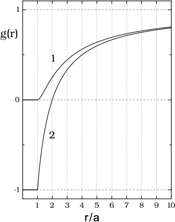
FIG. 1.: The pair distribution function for the hard-sphere bosons in the limit $n\to 0$: 1 - the data of Eq. (39); 2 - the result of the effective-interaction approach [5], Eq. (37). At $r<2a$ Eq. (37) yields unphysically negative values for $g(r)$.

As it is seen, at small particle separations $r\lesssim 3a$ the difference between the curves (1) and (2) is essential, while at large $r$ these curves are close to one another. We emphasize that the incorrect behaviour at the short distances is related to the modified Bogoliubov’s model [with the replacement $\Phi(k)\to 2\pi\hbar^{2}a/m$] but not to the original one developed for the case of a weakly interacting Bose gas.

The failure of the effective-interaction approach can be understood with the help of the interesting relation connecting the pair distribution function with the in-medium pair wave functions and following from the Bogoliubov principle of the correlation weakening [15, 16, 17]. We remind that the pair wave functions, by definition, are the eigenfunctions of the reduced density matrix of the second order. For the Bose gas, a system with a small condensate depletion $(n-n_{0})/n\ll 1$, the pair distribution function can be written as

$$g(r)=\left(\frac{n_{0}}{n}\right)^{2}\varphi^{2}(r)+2\frac{n_{0}}{n}\int\frac{\mbox{d}^{3}q}{(2\pi)^{3}}\frac{n_{q}}{n}\varphi^{2}_{{\bf q}/2}({\bf r}),$$ (41)

which is accurate to the next-to-leading order in $(n-n_{0})/n$ [18]. Another restriction for this representation is an assumption that there are no bound pair states (see details in Ref. [15]). In Eq. (41) $\varphi(r)$ is the in-medium pair wave function of two condensed bosons; $n_{q}=\langle a_{{\bf q}}^{\dagger}a_{{\bf q}}\rangle$; the quantity $\varphi_{{\bf q}/2}({\bf r})$ denotes the in-medium wave function of the relative motion of the pair of bosons with the total momentum $\hbar{\bf q}$. This pair includes one condensed and one uncondensed particle. The functions $\varphi(r)$ and $\varphi_{{\bf q}/2}({\bf r})$ are chosen as real quantities. It is also convenient to introduce the in-medium scattering waves $\psi(r)$ and $\psi_{{\bf p}}({\bf r})\;(p\not=0)$ given by

$$\varphi(r)=1+\psi(r),\;\varphi_{{\bf p}}({\bf r})=\sqrt{2}\cos({\bf p}{\bf r})+\psi_{{\bf p}}({\bf r})$$ (42)

with the boundary conditions at $r\to\infty$

$$\psi(r),\;\psi_{{\bf p}}({\bf r})\to 0.$$ (43)

The Fourier transforms of the scattering waves can be expressed in terms of the Bose operators $a_{{\bf p}}^{\dagger}$ and $a_{{\bf p}}$ [15]:

$$\psi(k)=\frac{\langle a_{{\bf k}}a_{-{\bf k}}\rangle}{n_{0}},\ {\psi}_{\bf p}({\bf k})=\sqrt{\frac{V}{2n_{0}}}\frac{\langle a^{\dagger}_{2{\bf p}}a_{{\bf p}+{\bf k}}a_{{\bf p}-{\bf k}}\rangle}{n_{2p}}.$$ (44)

At $n\to 0$ the in-medium pair wave functions tend to solutions of the ordinary two-body problem. For example, $\varphi(r)\to\varphi^{(0)}(r)$. Hence, as the condensate depletion $(n-n_{0})/n$ approaches zero when $n\to 0$, Eq. (41) is reduced to the Bogoliubov’s equation (39). A weakly interacting Bose gas is characterized by a minor role of the particle scattering, so that $|\psi(r)|\ll 1$ and $|\psi_{{\bf p}}({\bf r})|\ll 1$. In particular, the Bogoliubov model of a weak-coupling Bose gas implies $\psi_{{\bf p}}({\bf r})=0$ [15, 16], while $\psi(r)\not=0$. Thus, within the Bogoliubov model, Eq. (41) can be approximated as

$$g(r)=1+2\psi(r)+\frac{2}{n}\int\frac{\mbox{d}^{3}k}{(2\pi)^{3}}n_{k}\exp(i{\bf k}{\bf r}),$$ (45)

where the terms of the order of $(n-n_{0})^{2}/n^{2}$ and $\psi(r)(n-n_{0})/n$ have been ignored. At $n\to 0$ one can find [10, 16]

$$g(r)\to 1+2\psi^{(0)}_{B}(r),$$ (46)

where $\psi^{(0)}_{B}=\varphi^{(0)}_{B}(r)-1$ obeys the equation

$$-\frac{\hbar^{2}}{m}\nabla^{2}\varphi^{(0)}_{B}(r)+\Phi(r)=0,$$ (47)

which is the two-body Schrödinger equation (16) taken in the Born approximation. We stress that Eqs. (45)-(47) are related to the original Bogoliubov model. As to the modified Bogoliubov approach with the $t$ matrix, it produces Eq. (37). Now we are able to explain the failure of the effective-interaction scheme. The replacement of the original interaction $\Phi(k)$ by the $t$ matrix leads to passage from $\psi^{(0)}_{B}(r)$ to $\psi^{(0)}(r)$. However, it does not influence the Bogoliubov ansatz (45) for the relation between the pair distribution function and the pair wave functions. Substituting $\psi(k)=\langle a_{{\bf k}}a_{-{\bf k}}\rangle/n_{0}$ and $n_{k}=\langle a^{\dagger}_{{\bf k}}a_{{\bf k}}\rangle$ in Eq. (45) and using Eq. (24), one can see that the approximation (45) is consistent with the approximation (27) for the Green function (25). Thus, the effective-interaction scheme combines the features of both the strong- and weak-coupling regimes, and this is the actual reason for its problems discussed in the previous sections. In particular, the ultraviolet divergence does come from the double account mentioned in Sec. I, but our analysis reveals that the double account, in turn, is a consequence of the combination just pointed out. Note that the thermodynamic inconsistency of the modified Bogoliubov model, found in our previous publications [10, 16], results from this combination, too.

V Strong-coupling generalization of the Bogoliubov model

It follows from the consideration given above that in the strong-coupling regime one should leave the effective-interaction approach and develop a new one. What way should one prefer? At present the authors have no final solution providing the solid theoretical scheme and making it possible to realize systematic calculations like in the weak-coupling case. However, we can propose a reasonable strong-coupling generalization of the Bogoliubov model based on Eq. (41) and semi-phenomenological relation (49) discussed below. This generalization is justified as it reproduces the result of Lee and Yang (4), gives correct picture of the short-range particle correlations, and yields Eqs. (21) and (22). Besides, the way proposed provides self-consistent calculations of the in-medium pair wave functions approaching solutions of the ordinary two-body problem at $n\to 0$. The model considered below is similar to the Brueckner theory (see Secs. 36 and 41 in Ref. [19]) but with one advantageous exception. The point is that the Brueckner theory implies the momentum distribution of interacting particles to be the same as in an ideal gas. As to our model, it results in a system of equations connecting the in-medium pair wave functions with the momentum distribution.

In addition to Eq. (41), the proposed strong-coupling generalization of the Bogoliubov model involves two other relations. The first is the familiar expression for the mean energy per particle

$$\varepsilon=\int\frac{\mbox{d}^{3}k}{(2\pi)^{3}}T_{k}\frac{n_{k}}{n}+\frac{n}{2}\int\mbox{d}^{3}r\,g(r)\Phi(r),$$ (48)

which can be found in any textbook on statistical mechanics. The second is, say, the semi-phenomenological relation that connects the scattering waves (42) with the momentum distribution $n_{k}$:

$$n_{k}(n_{k}+1)=n_{0}^{2}{\psi}^{2}(k)+2n_{0}\int\frac{\mbox{d}^{3}q}{(2\pi)^{3}}n_{q}{\psi}^{2}_{{\bf q}/2}({\bf k}).$$ (49)

It is worth saying several words about Eq. (49). This equation represents, in particular, the well-known fact that when there is no scattering [interaction] in the system, there are no uncondensed bosons $n_{k}=0$ [20]. The larger interaction, the larger depletion of the Bose condensate. Equation (49) generalizes the similar relation of the Bogoliubov model given by (see Refs. [10, 16])

$$n_{k}(n_{k}+1)=n^{2}{\psi}^{2}(k).$$ (50)

The generalization (49) has been chosen in [10, 16] for the following reasons. First, it provides the relation $\sqrt{2}\psi(r)=\lim_{p\to 0}\psi_{{\bf p}}({\bf r})$ as well as

$$\sqrt{2}\varphi(r)=\lim_{p\to 0}\varphi_{{\bf p}}({\bf r}),$$ (51)

which can be inferred from Eqs. (42) and (43). Second, it leads to the correct thermodynamics and behaviour of $g(r)$ at short distances for a dilute Bose gas in the leading and next-to-leading orders in $na^{3}$. Third, the relation (49) results in Eq. (61) that gives not only short-range but also correct long-range behaviour of $\varphi(r)$. A shortcoming of this generalization is that it may be not unique, but it is the simplest one that provides the points mentioned above.

Equations (41) and (48) make it possible to express $\varepsilon$ in terms of the pair wave functions and momentum distribution. So, a variational procedure can be employed to determine these quantities. Perturbing ${\psi}(k)$ and $n_{k}$ and bearing in mind (49), from Eqs. (41) and (48) we find the following equation [16]:

$$-2\widetilde{T}_{k}{\psi}(k)={U}(k)\bigl{[}1+2\bigl{(}n_{k}+n{\psi}(k)\bigr{)}\bigr{]},$$ (52)

where $\psi(k)$ and $\psi_{{\bf p}}({\bf k})$ are the Fourier transforms of the scattering waves (42). Here ${U}(k)$ and $\widetilde{T}_{k}$ are defined by

$${U}(k) = \int\mbox{d}^{3}r\,\varphi(r)\Phi(r)\exp(-i{\bf k}{\bf r}),$$ (53)

$$\widetilde{T}_{k} = T_{k}+nt_{k},$$ (54)

where $t_{k}=U^{\prime}(k)-U(k)$ and

$$U^{\prime}(k) = \int\mbox{d}^{3}r\,\bigl{(}\varphi_{{\bf k}/2}^{2}({\bf r})-\varphi^{2}(r)\bigr{)}\Phi(r)$$ (56)

$$-\int\frac{\mbox{d}^{3}q}{(2\pi)^{3}}\frac{{U}(q)\bigl{(}{\psi}^{2}_{{\bf k}/2}({\bf q})-{\psi}^{2}(q)\bigr{)}}{{\psi}(q)}.$$

Note that $t_{k}\propto k^{4}$ for $k\to 0$ [16], and $\widetilde{T}_{k}/T_{k}\to 1$ when $k\to\infty$. So, at low momenta and small densities we have $nt_{k}\ll T_{k}$. Owing to this property the difference between $T_{k}$ and $\widetilde{T}_{k}$ does not play a role when calculating the first two terms of the low-density expansions for the basic thermodynamic quantities. Therefore, at sufficiently small values of $n$ Eq. (52) is reduced to

$$\frac{\hbar^{2}}{m}\nabla^{2}\varphi(r) = \varphi(r)\Phi(r)$$ (58)

$$+n\int\mbox{d}^{3}y\,\varphi(y)\Phi(y)\bigl{(}g_{tr}(|{\bf r}-{\bf y}|)-1\bigr{)},$$

where $g_{tr}(r)$ stands for the truncated pair distribution function that is equal to the right-hand side of Eq. (45) even beyond the weak-coupling regime. Equation (58) is very similar to the Bethe-Goldstone equation [21]. However, there is also difference between them. Indeed, $g_{tr}$ depends not only on the scattering wave $\psi(k)$ but on the momentum distribution $n_{k}$, too. While the Bethe-Goldstone equation involves one unknown, the pair wave function.

Equations (41) and (49) are accurate to the next-to-leading order in $(n-n_{0})/n$, then, Eq. (52) can be accurate only to the leading order in $(n-n_{0})/n$. So, to find $\psi(k)$ and $n_{k}$, one should solve Eq. (52) in conjunction with Eq. (49) taken in the approximation valid to the leading order in the condensate depletion. In other words, one has to consider the system of Eqs. (50) and (52) which has the following solution:

$$n_{k} = \frac{1}{2}\Biggl{(}\frac{\widetilde{T}_{k}+nU(k)}{\sqrt{\widetilde{T}_{k}^{2}+2n\widetilde{T}_{k}U(k)}}-1\Biggr{)},$$ (59)

$$\psi(k) = -\frac{1}{2}\frac{U(k)}{\sqrt{\widetilde{T}_{k}^{2}+2n\widetilde{T}_{k}U(k)}}.$$ (60)

Note that as to the scattering states of a pair made of one condensed and one uncondensed boson, the goal of the present investigation makes it possible not to go into details. Below it is only sufficient to limit ourselves to the relation (51).

In the zero-density limit, Eq. (60) is reduced to ${\psi}(k)=\psi^{(0)}(k)=-{U}^{(0)}(k)/(2T_{k})$, which can be rewritten in the form of Eq. (16). So, at sufficiently small densities we can express the quantities ${\psi}(k)$ and $n_{k}$ in terms of the vacuum scattering amplitude ${U}^{(0)}(k)$ given by Eq. (15) [in the Beliaev’s notations ${U}^{(0)}(k)=f({\bf k},0)$]. This is totally consistent with the well-known argument of Landau [22] according to which the thermodynamics of dilute quantum gases is determined by the vacuum scattering amplitude. Note that the expressions for ${\psi}(k)$ and $n_{k}$ derived within the original Bogoliubov model can be obtained [10, 16] from Eqs. (59) and (60) with replacement of $\widetilde{T}_{k}$ and ${U}(k)$ by $T_{k}$ and ${\Phi}(k)$, respectively. So, in what concerns the expressions for $n_{k}$ and $\psi(k)$, the situation looks as if we operated with a Bose gas of weakly interacting quasiparticles with the renormalized kinetic energy $\widetilde{T}_{k}$ and effective interaction $U(r)=\varphi(r)\Phi(r)$. This is indeed close to the expectations based on the effective-interaction approach of the papers [5].

VI Short-range boson spatial correlations

Now, to elaborate on the picture of the short-range boson correlations, let us investigate how the correlation hole stipulated by the repulsion between bosons at small separations changes under the influence of the surrounding bosons. At $n\to 0$ this hole is completely specified by the condensate-condensate pair wave function $\varphi(r)$, which can be found from the definition (53). Using this definition and Eq. (60), for the scattering amplitude one can find

$${U}(k)={\Phi}(k)-\frac{1}{2}\int\frac{\mbox{d}^{3}q}{(2\pi)^{3}}\frac{{\Phi}(|{\bf k}-{\bf q}|){U}(q)}{\sqrt{\widetilde{T}^{2}_{q}+2n\widetilde{T}_{q}{U}(q)}},$$ (61)

which is the in-medium Lippmann-Schwinger equation. Let us rewrite Eq. (61) in the form

$${U}(k)={\Phi}(k)-\frac{1}{2}\int\frac{\mbox{d}^{3}q}{(2\pi)^{3}}\frac{{\Phi}(|{\bf k}-{\bf q}|){U}(q)}{T_{q}}-I,$$

where for $I$ we have

$$I=\frac{1}{2}\int\frac{\mbox{d}^{3}q}{(2\pi)^{3}}\Biggl{[}\frac{{\Phi}(|{\bf k}-{\bf q}|){U}(q)}{\sqrt{\widetilde{T}^{2}_{q}+2n\widetilde{T}_{q}{U}(q)}}-\frac{\Phi(|{\bf k}-{\bf q}|){U}(q)}{T_{q}}\Biggr{]}.$$

Performing the “scaling” substitution

$${\bf q}={\bf q^{\prime}}\sqrt{2mn}/\hbar$$ (62)

in the integral and, then, taking the zero-density limit in the integrand, for $n\to 0$ we find [23]

$$I=-\alpha{\Phi}(k),\quad\alpha=\frac{\sqrt{nm^{3}}}{\pi^{2}\hbar^{3}}{U}^{3/2}(0).$$ (63)

From Eqs. (61) and (63) it now follows that

$$U(k)-{U} {}^{(0)}(k)=\alpha{\Phi}(k)$$ (65)

$$-\int\frac{\mbox{d}^{3}q}{(2\pi)^{3}}\frac{{\Phi}(|{\bf k}-{\bf q}|)}{2T_{q}}\bigl{[}{U}(q)-{U}^{(0)}(q)\bigr{]},$$

where $U^{(0)}(k)$ obeys Eq. (61) with $n=0$, i.e. the standard Lippmann-Schwinger equation. Introducing the quantity ${\xi}(q)=-[{U}(q)-{U}^{(0)}(q)]/(2T_{q})$, for its Fourier transform $\xi(r)$ we find the equation that is nothing else but the Schrödinger equation (16) with $\varphi^{(0)}(r)$ replaced by $\alpha+\xi(r)$. As $\xi(r)\to 0$ when $r\to\infty$, we can conclude that $\xi(r)=\alpha\psi^{(0)}(r)$. Hence, for $n\to 0$ we get

$${U}(k)\simeq{U}^{(0)}(k)\left(1+\gamma(k,n)\frac{8}{\sqrt{\pi}}\sqrt{na^{3}}\,\right).$$ (66)

Here $\gamma(k,n)\to 1$ when $n\to 0$. At $k=0$ the derived result for, say, the in-medium scattering amplitude $U(k)$ coincides with the expansion in $na^{3}$ for the effective potential found within the effective-interaction approach at the zero temperature (see, e.g., the review [24], Eq. (4.27)). This shows once more that there are actual parallels between our model and approach of Ref. [5]. However, these parallels are accompanied by significant differences. First, the in-medium Lippmann-Schwinger equation (61) is not a variant of the $t$ matrix equation which is frequency dependent, contrary to Eq. (61). Second, Eq. (61) has been found beyond any diagram technique by means of the variational procedure. One of its important consequences is that the pair wave functions that “generate” the in-medium scattering amplitudes [see Eq. (53) and Eq. (74) below] in our approach coincide with the pair wave functions that make a contribution to $g(r)$ [see Eq. (41)]. By contrast, the modified Bogoliubov model implies the plane waves for $\varphi_{{\bf p}}({\bf r})$ ($p\not=0$) in the pair distribution function (45) (see Sec. IV), while one certainly goes beyond the plane-wave approximation when calculating $t$ matrix corresponding to a pair of particles with nonzero total momenta.

With the help of Eq. (66), at $n\to 0$ we obtain the following in-medium renormalization for $\varphi^{(0)}(r)$ at short distances:

$$\varphi(r)\simeq\varphi^{(0)}(r)\Bigl{(}1+\frac{8\sqrt{na^{3}}}{\sqrt{\pi}}\Bigr{)}.$$ (67)

Equation (67) is indeed a short-range approximation, and this can be understood from the fact that, at sufficiently large momenta $k$, the main contribution in the integral in the right-hand side of Eq. (61) comes from the large momenta $q$. As $\lim_{q\to\infty}U(q)/\widetilde{T}_{q}=0$, then for $k\to\infty$ Eq. (61) is also (like at $n\to 0$) reduced to the two-body Lippmann-Schwinger equation, and, thus, $\varphi(r)$ obeys the Schrödinger equation (16) at small boson separations. In order to explain the origin of the factor $C=1+8\sqrt{na^{3}}/\sqrt{\pi}$ in Eq. (67), we remind that the boundary conditions (43), involved implicitly in the in-medium Lippmann-Schwinger equation (61), are valid for $r\gg r_{0}$, where $r_{0}=n^{-1/3}$ is the mean distance between two particles in the gas. The wave function $\varphi(r)$, related to a couple of bosons in the Bose-Einstein condensate, does obey Eq. (16) at $r\to 0$, but it differs from $\varphi^{(0)}(r)$, subjected to the boundary condition (17), by the factor that is determined by the in-medium effects. Thus, the range of validity of Eq. (67) is restricted by the region $r\lesssim r_{0}$; in the vicinity of $r_{0}$ the behaviour of $\varphi(r)$ is rather complicated; and for $r\gg r_{0}$ the function $\varphi(r)$ is subjected to the following asymptotics:

$$\psi(r)=\varphi(r)-1\simeq-\frac{1}{2{\pi}^{3/2}}\sqrt{\frac{a}{n}}\frac{1}{r^{2}}.$$ (68)

The latter evaluation can be obtained from Eq. (60), which yields $\psi(k)\simeq-\sqrt{\pi a/n}/k$ for $k\to 0$, and at $r\to\infty$ we arrive at Eq. (68), contrary to the two-body problem, which implies $\psi^{(0)}(r)\simeq-a/r$. Thus, the unusual “overscreening” takes place for the wave function $\varphi(r)$ owing to in-medium effects.

Now we are able to calculate the pair distribution function for a dilute Bose gas from Eq. (41). By means of the substitution (62) in the integral in Eq. (41) one can rewrite the pair distribution function for $n\to 0$ in the form

$$g(r)\simeq\left(1+2\frac{n-n_{0}}{n}\right)\varphi^{2}(r).$$ (69)

where the relation (51) is implied. This is short-range approximation for $g(r)$, for the oscillating function $\cos({\bf k}{\bf r})$ makes an important contribution to the integral in Eq. (41) at large $r$. To obtain a more concrete information from Eq. (69), one should calculate the condensate depletion. It can be derived from Eq. (59) with the “scaling” substitution given by Eq. (62). This leads to

$$\frac{n-n_{0}}{n}=\int\frac{\mbox{d}^{3}q}{(2\pi)^{3}}\frac{n_{q}}{n}=\frac{8\sqrt{na^{3}}}{3\sqrt{\pi}}+\cdots$$ (70)

The result again coincides with that of the effective-interaction scheme because the momentum distribution (59) is very close to $n_{k}$ found within the modified Bogoliubov model. Rewriting Eq. (69) with the help of Eqs. (67) and (70), we arrive at the expression (38) that has earlier been obtained by means of the theorems (5) and (14). One can see that Eq. (38) is also violated at the mean distance between particles, $r_{0}$, since Eq. (67) for $\varphi(r)$ is broken when $r\gtrsim r_{0}$.

For strongly singular potentials, when $\varphi^{(0)}(r=0)=0$, the correct result $g(r=0)=0$ takes place according to Eq. (38). As one can see from (38), the correlation hole coming from the repulsion of bosons at small particle separations gets less marked with an increase of the density of the surrounding bosons, which is consistent with usual expectations concerning the particle spatial separations.

Now it is interesting to compare the result given by Eq. (38) with the data of the Monte-Carlo calculations for the hard-spheres [25]. With the two-body wave function (40) for the hard-sphere interaction (23), Eq. (38) reads

$$g(r)=\left\{\begin{array}[]{ll}0,&r\leq a\\ (1-a/r)^{2}[1+64\sqrt{na^{3}}/(3\sqrt{\pi})],&r>a.\end{array}\right.$$ (71)

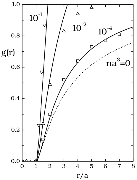
FIG. 2.: The pair distribution function corresponding to the hard-sphere potential (23) for various values of the gas parameter $na^{3}$. Solid lines – the data of Eq. (71); $\Box$, $\bigtriangleup$, $\bigtriangledown$ – the data of the Monte-Carlo calculations [25] for $na^{3}=10^{-4},\,10^{-2},\,10^{-1}$, respectively. The difference becomes significant at the mean distance between particles $r_{0}$, where $r_{0}/a=\left(na^{3}\right)^{-1/3}=21.5,\,4.64,\,2.15$, respectively. Dotted line – Eq. (71) for $na^{3}=0$, one can see that $g(r)$ is essentially changed even for small values of the gas parameter.

The results are displayed in Fig. 2 for various values of the gas parameter $na^{3}$. We remark that, strictly speaking, only the situation when $na^{3}=10^{-4}$ can be investigated with Eq. (71) because even at $na^{3}=10^{-2}$ we have $64\sqrt{na^{3}}/(3\sqrt{\pi})\approx 1.20$, so that the next-to-leading order in Eq. (38) makes contribution more essential than that of the leading order in $na^{3}$. However, as it is seen, the short-range approximation of Eq. (71) works well at small values of $r$ even at $na^{3}=10^{-1}$. This agrees with a conclusion of Giorgini et al. [25] that Eq. (4), derived to the next-to-leading order in $na^{3}$, provides results very close to the energy of a dilute Bose gas even at $na^{3}=10^{-1}$. Agreement of the data of the Monte-Carlo calculations with the results coming from Eq. (41) can be considered as the direct positive test supporting the expression (41), which is based on the Bogoliubov principle of correlation weakening in the strongly interacting Bose gas (see Ref. [15]).

Concluding this section, let us stress one more that Eqs. (67) and (38) are correct only for short boson separations. To determine the long- and intermediate-range behaviour of $g(r)$ with the aim, for example, of finding the structural factor $S(k)$ at all values of $k$, one should obtain $\varphi_{{\bf p}}({\bf r})$ for all values of ${\bf p}$ [remember that only the limiting relation (51) have been utilized]. This investigation is directly connected with the problem of the relation between the boson momentum distribution and pair scattering waves [see Eq. (49)] and needs additional extended considerations being beyond the scope of this paper. The same concerns the spectrum of elementary excitations. Now, and here the point is, this problem is much more complicated as compared to the Bogoliubov model (original or modified). Within the Bogoliubov approach the long-range behaviour of $g(r)$ is only governed by the two quantities $\psi(k)=\langle a_{{\bf k}}a_{-{\bf k}}\rangle/n_{0}$ and $n_{k}=\langle a^{\dagger}_{\bf k}a_{\bf k}\rangle$ [see Eq. (45)]. But now we have the rather complicated functional (41) of $n_{k}$, $\psi(k)$ and $\psi_{{\bf p}}({\bf k})$ given by Eq. (44).

VII Thermodynamics of a dilute Bose gas

After the necessary preparations, we are able to turn to the thermodynamics of a strong-coupling Bose gas. The most simple way of doing so is to deal with the chemical potential $\mu$ starting from the well-known relation

$$\mu=\frac{1}{\sqrt{n_{0}}}\int\mbox{d}^{3}r^{\prime}\,\Phi(|{\bf r}-{\bf r}^{\prime}|)\langle\psi^{\dagger}({\bf r}^{\prime})\psi({\bf r}^{\prime})\psi({\bf r})\rangle,$$ (72)

valid in the presence of the Bose condensate [26]. Here $\psi^{\dagger}({\bf r})$ and $\psi({\bf r})$ stand for the Bose field operators. This relation follows from the expression for the infinitesimal change of the grand canonical potential $\delta\Omega=\langle\delta(\hat{H}-\mu\hat{N})\rangle$ and the necessary condition of the minimum for $\Omega$ with respect to the order parameter $N_{0}$: $\partial\Omega(N_{0},\mu,T)/\partial N_{0}=0$, the Hamiltonian depending on the number of the condensed particles owing to the substitution $a_{0}^{\dagger}=a_{0}=\sqrt{N_{0}}$. Equations (44) and (72) lead to

$$\mu=n_{0}{U}(0)+\sqrt{2}\int\frac{\mbox{d}^{3}q}{(2\pi)^{3}}n_{q}{U}_{{\bf q}/2}({\bf q}/2),$$ (73)

where the quantity

$${U}_{{\bf p}}({\bf k})=\int\mbox{d}^{3}r\,\varphi_{\bf p}({\bf r})\Phi(r)\exp(-i{\bf k}{\bf r})$$ (74)

is introduced. The quantities $U(k)$ and ${U}_{{\bf p}}({\bf k})$, which can be called the in-medium scattering amplitudes, differ from $f({\bf k},{\bf k}^{\prime})$ introduced by Beliaev. The latter is determined by the solutions of the ordinary two-body problem with the boundary conditions corresponding to the usual plane-waves for $r\to\infty$. As to $U(k)$, it is determined from the in-medium Lippmann-Schwinger equation (61). In order to obtain the next-to-leading order for $\mu$, it is sufficient to use the relation $\sqrt{2}U(k)=\lim_{p\to 0}{U}_{{\bf p}}({\bf k})$, which follows from Eq. (51). In this way, employing the substitution (62) in the integral and taking into consideration Eqs. (15), (66) and (70), we can rewrite Eq. (73) for $n\to 0$ in the form

$$\mu = nU(0)\left(1+\frac{n-n_{0}}{n}+\cdots\right)$$ (75)

$$= \frac{4\pi\hbar^{2}an}{m}\left(1+\frac{32}{3\sqrt{\pi}}\sqrt{na^{3}}+\cdots\right).$$ (76)

Equation (76), together with the thermodynamic relation $\mu=\partial(n\varepsilon(n))/\partial n$, yields the Yang-Lee’s result (4).

It is worth noting that we can also use the direct way of calculating $\varepsilon$ based on Eq. (48). However, one could come to a wrong conclusion if Eq. (48) employed in conjunction with Eq. (50). To use this way, one should go beyond Eq. (50) and take into account the density correction to that relation,

$$n_{k}(n_{k}+1)=\left(1+2\frac{n-n_{0}}{n}\right)\psi^{2}(k),$$ (77)

following from Eq. (49) at $n\to 0$. Thus, the preliminary result found in Ref. [16] should be abandoned in favour of Eq. (4).

The correct behaviour of the pair distribution function found in the previous section allows for deriving the correct results for the kinetic and interaction energies by a direct calculation, even beyond the Hellmann-Feynman theorem. For example, substituting Eq. (38) into Eq. (7) and taking account of Eq. (19), one can immediately find Eq. (21).

VIII Conclusion

In conclusion, we remark that the present paper deals with the thermodynamics of a Bose gas of strongly interacting particles in the leading and next-to-leading orders of the expansion in $na^{3}$. The strong-coupling generalization of the Bogoliubov model considered here reproduces the well-known formula of Lee and Yang (4) and, contrary to the effective-interaction approach of Ref. [5], yields correct results for the kinetic and interaction energies and short-range spatial correlations of bosons. To go further, additional investigations should be fulfilled. In particular, it is necessary to solve the problem concerning the relation that connects the boson momentum distribution with the scattering waves. The spectrum of the elementary excitations should also be considered within the approach of Refs. [10, 15, 16] in order clarify to what extent it differs from the well-known prediction of the effective-interaction approach. We, of course, mean the region of intermediate momenta rather than the linear phonon part, which should be the same according to the thermodynamic prescription. This question can not be answered without addressing the long-range spatial boson correlations.

The authors are grateful to S. Giorgini for making the data of the Monte-Carlo calculations [25] available to us. This work was supported by the RFBR grant No. 00-02-17181.

REFERENCES

- [1] E-mail: cherny@thsun1.jinr.ru
- [2] E-mail: shanenko@thsun1.jinr.ru
- [3] M. H. Anderson, J. R. Enscher, M. R. Matthews, C. E. Wieman, and E. A. Cornell, Science 269, 198 (1995); K. B. Davis, M.-O. Mewes, M. R. Andrews, N. J. van Druten, D. S. Durfee, D. M. Kurn, and W. Ketterle, Phys. Rev. Lett. 75, 3969 (1995); C. C. Bradley, C. A. Sackett, J. J. Tollett, and R. G. Hulet, ibid 75, 1687 (1995); C. C. Bradley, C. A. Sackett, and R. G. Hulet, ibid. 78, 985 (1997).
- [4] F. Dalfovo, S. Giorgini, L. P. Pitaevskii, and S. Stringari, Rev. Mod. Phys. 71, 463 (1999); A. S. Parkins and D. F. Walls, Phys. Rep. 303, 1 (1998).
- [5] T. D. Lee, K. Huang, and C. N. Yang, Phys. Rev. 106, 1135 (1957); K. A. Brueckner and K. Sawada, Phys. Rev. 106, 1117 (1957); S. T. Beliaev, Zh. Exp. Teor. Fiz. 34, 433 (1958) [Sov. Phys. JETP 7, 299 (1958)]; N. M. Hugenholtz and D. Pines, Phys. Rev. 116, 489 (1959) [for recent situation see E. Braaten and A. Nieto, Eur. Phys. J. B 11, 143 (1999)].
- [6] We employ the following classification of the short-range pairwise potentials. The potential is of weak-coupling type if it is integrable and proportional to a small parameter. In this case the Born approximation works well in the ordinary two-body problem, and, hence, in the Born series (2) . Otherwise the potential is called singular. Finally, we deals with the strongly singular potential (strong coupling regime) if the individual terms in Eq. (2) do not exist due to strong repulsion at short distances. For example, the potential at or the hard-sphere potential (23) belongs to that type.
- [7] N. N. Bogoliubov, J. Phys. (USSR) 11, 23 (1947), reprinted in Ref. [9].
- [8] P. Nozières and D. Pines, Nuovo Cimento IX, 470 (1958).
- [9] D. Pines, ed., The many-body problem (W.A. Benjamin, New York, 1961), p. 76.
- [10] A. Yu. Cherny and A. A. Shanenko, Journal of Phys. Stud. (Ukraine) 3, 272 (1999), the Issue in memory of academician Bogoliubov; cond-mat/9904217.
- [11] T. D. Lee and C. N. Yang, Phys. Rev. 105, 1119 (1957).
- [12] W. Ketterle and H.- J. Miesner, Phys. Rev. A 56, 3291 (1997); A. Minguzzi, P. Vignolo, and M. P. Tosi, Phys. Rev. A 62, 023604 (2000).
- [13] E. H. Lieb and J. Yngvason, Phys. Rev. Lett. 80, 2504 (1998).
- [14] Here the ordinary scattering problem for particles with the mass ( denotes the mass of the boson) is implied so that tends to as . Whereas the pair wave functions used in Secs. IV-VII are symmetrized with respect to the boson permutation and, thus, obey the boundary conditions (42) and (43). So, the scattering amplitude used below is not the same as and this is by two reasons. First, it is due to symmetrization of the pair wave functions. Second, is governed by the in-medium pair wave functions.
- [15] A. Yu. Cherny, cond-mat/9807120.
- [16] A. Yu. Cherny and A. A. Shanenko, Phys. Rev. E 60, R5 (1999).
- [17] A. Yu. Cherny and A. A. Shanenko, Phys. Rev. B 60, 1276 (1999).
- [18] By the leading order in we mean the zero depletion of the condensate: .
- [19] A. L. Fetter and J. D. Walecka, Quantum theory of many-particle systems (McGraw-Hill, New York, 1971).
- [20] It is not, of course, the case at nonzero temperatures.
- [21] H. A. Bethe and J. Goldstone, Proc. R. Soc. London, Ser. A 238, 551 (1957).
- [22] See the footnote in Ref. [7].
- [23] This is possible as after the “scaling” substitution the integral uniformly converges for with respect to the parameter for .
- [24] H. Shi and A. Griffin, Phys. Rep. 304, 1 (1998).
- [25] S. Giorgini, J. Boronat, and J. Casulleras, Phys. Rev. A 60, 5129 (1999).
- [26] N. N. Bogoliubov, Lectures on quantum statistics, Vol. 2 (Gordon and Breach, New York, 1970), p. 1.