Is the quantum dot at large bias a weak-coupling problem?

Abstract

We examine the two-lead Kondo model for a d.c. biased quantum dot in the Coulomb blockade regime. From perturbative calculations of the magnetic susceptibility, we show that the problem retains its strong-coupling nature, even at bias voltages larger than the equilibrium Kondo temperature. We give a speculative discussion of the nature of the renormalization group flows and the strong-coupling state that emerges at large voltage bias.

For over a decade, transport measurements on quantum dot systems have stimulated theoretical interest in the properties of the Anderson model out of equilibrium Kastner:1993 ; Meirav:1996 ; Ashoori:1996 . Early predictions Glazman:1988 ; Ng:1988 ; Meir:1992 ; Meir:1993 ; Wingreen:1994 ; Konig:1996 of the Kondo effect in such systems have recently been experimentally verified GG:1998 ; Cronenwett:1998 ; Schmid:1998 ; vanderWiel:2000 . In the small voltage regime, such experiments have produced impressive agreement with theoretical predictions. Recent interest Glazman:2000 ; Langreth ; Schiller:1998 has turned to the question of how the Kondo effect behaves far from equilibrium, i.e. at large voltage bias.

In the Coulomb blockade regime, one may neglect charge fluctuations of a quantum dot and concentrate on transport processes that operate by flipping the dot’s spin. In this limit, the physics is described by a two-lead Kondo model Avishai:1998 ; Glazman:2000 (eq. (1)). A key property of the Kondo model in equilibrium is the presence of a “running coupling constant”, whereby the antiferromagnetic coupling between the dot spin and the leads grows as the energy scale is reduced. This leads to a “strong coupling” low-energy regime where the spin of the dot is quenched by the lead electrons and the residual properties can no longer be obtained from a perturbative expansion. A single scale, the “Kondo temperature” $T_{K}$, governs the low temperature properties; $T_{K}=D\sqrt{g}\,e^{-1/2g}$, where $g$ is the ‘bare coupling’ between the spin of the dot and the leads and $D\,{\gg}\,T_{K}$ is the electron bandwidth. Thus the magnetization at temperature $T$ and magnetic field $B$ is a universal function $M=m(T/T_{K},B/T_{K})$, where $M$ has a perturbative “weak coupling” expansion in $g$ only when $T,B\gg T_{K}$. (See Fig. 1(a).)

In a quantum dot, the formation of an Abrikosov-Suhl resonance in the quasiparticle density of states which accompanies the Kondo effect substantially enhances the linear conductivity at low temperature, resulting in unitary transmission at absolute zero Glazman:1988 ; Ng:1988 .

Figure 1: (a) Field dependence of the crossover temperature $T_{K}^{*}(B)$ separating weak- and strong-coupling regimes of the equilibrium Kondo model. At absolute zero, for fields larger than the Kondo temperature the quantum dot re-enters weak coupling. (b) Voltage dependence of the crossover temperature $T_{K}^{*}(V)$, from our results. Note that $T_{K}^{*}$ goes to zero only in the limit $V\to\infty$, i.e. for low enough temperatures, the model reaches a strong coupling state for all $V$.

But what happens to the physics of the quantum dot at voltages $V$ comparable to or larger than the Kondo temperature? In particular, does a large voltage act like a large magnetic field or temperature, and return the dot to a weak coupling regime where its spin is unquenched? Theoretical studies of the differential conductivity $G[V]$ do suggest that the large voltage physics is governed by weak-coupling perturbation theory, for Glazman:2000 $G=(2e^{2}/h)F[eV/T_{K}]$ has a perturbative expansion in $g$ for $V\gg T_{K}$. However, the large bias conductivity probes electrons that are far from the Fermi surface and does not in itself shed light on the coupling between the local moment and the electrons near the Fermi surface.

In this letter, we argue that the quantum dot retains its strong-coupling character even at voltages $V\gg T_{K}$. We use explicit perturbative calculations of the magnetic susceptibility to show that the large bias quantum dot is characterized by a strong-coupling regime with a voltage-dependent Kondo temperature $T_{K}^{*}\propto T_{K}^{2}/eV$.

The Hamiltonian of the two-lead Kondo model is

$$H = \sum_{\alpha{\bf k}\sigma}\varepsilon_{\alpha{\bf k}}c^{\dagger}_{\alpha{\bf k}\sigma}c_{\alpha{\bf k}\sigma}+H_{\rm refl}+H_{\rm trans};$$ (1)

$$H_{\rm refl} = J_{R}\sum_{{\bf k},{\bf k}^{\prime},\sigma,\sigma^{\prime}}\left(c^{\dagger}_{R{\bf k}\sigma}{\vec{\sigma}}_{\sigma\sigma^{\prime}}c_{R{\bf k}^{\prime}\sigma^{\prime}}\right)\cdot{\vec{S}}\,\,+\,\,(R\to L),$$

$$H_{\rm trans} = J_{LR}\sum_{{\bf k},{\bf k}^{\prime},\sigma,\sigma^{\prime}}\left(c^{\dagger}_{R{\bf k}\sigma}{\vec{\sigma}}_{\sigma\sigma^{\prime}}c_{L{\bf k}^{\prime}\sigma^{\prime}}\right)\cdot{\vec{S}}\,\,+\,\,(R\leftrightarrow L).$$

Here, $c^{\dagger}_{\alpha{\bf k}\sigma}$ creates an electron in lead $\alpha\in\left\{L,R\right\}$ with momentum ${\bf k}$ and spin $\sigma$, and $J_{L}$, $J_{R}$ and $J_{LR}=J_{RL}$ are positive (antiferromagnetic) Kondo coupling constants between the electrons and the dot ($\vec{S}$).

The first part of $H$ describes the electrons in the leads, with energies $\varepsilon_{\alpha{\bf k}}=\varepsilon_{{\bf k}}-eV_{\alpha}$, where $V_{\alpha}=\pm V/2$ are the potentials of the left- and right-hand leads. $H_{\rm refl}$ describes regular Kondo processes, where an electron from a given lead is spin-flip scattered back into the same lead; $H_{\rm trans}$ describes ‘spin-flip cotunnelling’, where an electron from one lead is spin-flip scattered into the other lead. We introduce the dimensionless couplings ${\bar{J}}_{L},{\bar{J}}_{R},{\bar{J}}_{LR}$, defined by ${\bar{J}}_{i}\equiv\rho J_{i}$, where $\rho$ is the density of states at the Fermi levels. When the model is derived from an Anderson model via a Schrieffer-Wolff transformation Schrieffer:1966 ; Kaminski:1999 , the coupling constants obey $|J_{LR}|^{2}=J_{L}J_{R}$, restricting the scattering to a single channel. Symmetric dots ($J_{L}{=}J_{R}{=}J_{LR}$), are of particular interest, for in this case the differential conductivity $G$ approaches the unitary limit ($2e^{2}/h$) at low temperatures.

In a magnetic field we replace $H\rightarrow H-BM_{z}$, where $M_{z}=2S_{z}+\sum_{\alpha{\bf k}\sigma}\sigma n_{\alpha{\bf k}\sigma}$ is the magnetization. The impurity susceptibility is ${\chi}_{i}=\frac{\partial}{\partial B}M_{z}|_{B=0}-\chi_{o}$, where $\chi_{o}=4\rho$ is the Pauli susceptibility of the leads. We expand $\chi_{i}$ perturbatively to order $J^{2}$ using the Keldysh method Rammer:1986 , and representing the spin as ${\vec{S}}=-{i\over 2}{\vec{\eta}\times\vec{\eta}}$, where the elements of ${\vec{\eta}}$ are Majorana fermions. In the large-bandwidth limit we find that

$$\chi_{i}=\frac{1}{T}\left\{1-\frac{1}{2}(\bar{J}_{R}+\bar{J}_{L})-\left(\bar{J}_{L}^{2}+\bar{J}_{R}^{2}\right)\ln\left(\frac{D}{2\pi Te^{1+\gamma}}\right)\right.\\ \left.-2|\bar{J}_{LR}|^{2}\left[\ln\left(\frac{D}{2\pi Te^{1+\gamma}}\right)-\phi\left(\frac{V}{T}\right)\right]\right\}.$$ (2)

where $\gamma=0.577\dots$ is the Euler constant. The crossover function $\phi(x)$, in terms of digamma functions $\psi(z)$, is

$$\phi(x)=\hbox{Re}\int_{-\infty}^{\infty}\frac{dy}{4\cosh^{2}\bigl{(}\frac{y}{2}\bigr{)}}\left[\tilde{\psi}(y+x)-\tilde{\psi}(y)\right]$$ (3)

where $\tilde{\psi}(x)=\psi(\frac{1}{2}+i\frac{x}{2\pi})$.

The second-order terms in (2) describe the leading logarithmic enhancement of the Kondo coupling. Terms of order $J_{LR}^{2}$ involve inter-lead processes and, as expected, the logarithmic divergence in these terms is cut by the voltage. (To see this, note that $-\phi(V/T)\sim-\ln(V/T)$ for $V\gg T$ which cancels the logarithmic temperature divergence.) By contrast, the intra-lead terms of order $J_{R}^{2}$ and $J_{L}^{2}$ are completely unaffected by the voltage $V$, which guarantees that the leading logarithmic divergence survives at arbitrarily high voltage. This is easily seen in the large-$V$ form of the susceptibility,

$$\chi_{i}=\frac{1}{T}\left\{1-\frac{1}{2}(\bar{J}_{R}+\bar{J}_{L})-\left(\bar{J}_{L}^{2}+\bar{J}_{R}^{2}\right)\ln\left(\frac{D}{2\pi Te^{1+\gamma}}\right)\right.\\ \left.-2|\bar{J}_{LR}|^{2}\ln\left(\frac{D}{V}\right)\right\},\qquad\quad V\gg T.$$ (4)

The survival of these leading logarithms is a signature that the intra-lead Kondo effect continues unabated at temperatures smaller than the voltage.

Let us now be more precise by defining a generalized crossover temperature $T_{K}^{*}$ as the temperature below which the perturbation expansion (2) breaks down, i.e. the temperature at which the $O(J)$ and $O(J^{2})$ terms become equal in magnitude. This procedure yields an implicit formula for $T^{*}_{K}(V)$

$$T^{*}_{K}(V)=T_{K}e^{-\frac{1}{2}\phi(V/T_{K}^{*}(V))}$$ (5)

where $T_{K}=De^{-1/2g}$ is the leading approximation to the Kondo temperature note . We plot $T_{K}^{*}(V)$ in Fig. 1(b).

Note that $T_{K}^{*}$ goes to zero only when $V$ goes to infinity. From the behavior of $\phi$ at large argument, we can extract the large voltage behavior

$$T^{*}_{K}=\frac{(T_{K})^{2}}{V}.$$ (6)

This means that the model always enters a strong coupling regime at low temperature, even for $V\gg T_{K}$.

These perturbative results for $\chi_{i}$ may be interpreted within a simple renormalization picture. Let us stress, however, that there is not yet a general theory of renormalization out of equilibrium (though see Schoeller ). In particular, it has not been established that there exists an appropriate family of effective Hamiltonians through which one passes as the high-energy cutoff scale is varied. Furthermore, in the presence of a voltage, long-time processes cannot be unambiguously connected with low-energy ones. Hence the following discussion is somewhat speculative, and steps beyond the perturbative calculation that led to (5).

In the spirit of a “poor man’s scaling” approach poor , we consider varying a cutoff energy scale $\Lambda$ in the problem, and studying the variation of the effective coupling constants $J_{L},J_{R},J_{LR}$ as functions of this variable. The essential scaling behavior, as usual, can be read off from the perturbative expression (2). We may identify two scaling regimes:

(1) One-channel scaling, $\Lambda\gg V$. In this regime the effect of the voltage is not felt in any channel, so the dot behaves as an equilibrium single-channel Kondo model. The single coupling constant $g\equiv{\bar{J}}_{L}+{\bar{J}}_{R}$ rescales according to

$$\frac{dg}{d\ln\Lambda}=-2g^{2}+O(g^{3})$$ (7)

so to leading order in the scaling, the coupling constant at scale $\Lambda=V$ is given by $\frac{1}{g^{*}}=\frac{1}{g}-2\ln(D/V)$. In this regime, the ratio $J_{LR}/g$ is preserved.

(2) Two-channel regime $V\gg\Lambda\gg T^{*}_{K}(V)$. Around $\Lambda\sim V$ the logarithmic renormalization of inter-lead processes comes to a halt, freezing $J_{LR}$ at its value $J_{LR}(V)$ and prompting a crossover to a two-channel scaling regime in which intra-lead processes independently renormalize $J_{R}$ and $J_{L}$. This scenario is reminiscent of one proposed by Wen Wen:1998 : that the effect of the voltage is to destroy coherence between the two leads, suppressing the $J_{LR}$ terms, and leaving a two-channel Kondo Hamiltonian. We shall restrict our attention to symmetric dots, so that $J_{L,R}=\bar{J}(\Lambda)$ scale together according to

$$\frac{d{\bar{J}}}{d\ln\Lambda}=-2{{\bar{J}}\,}^{2}+O({{\bar{J}}\,}^{3}).$$ (8)

At voltage $V$, ${\bar{J}}_{R,L}=g^{*}/2$, so to leading order, the coupling constants are given by

$$\frac{1}{{\bar{J}}(\Lambda)}=\frac{2}{{g^{*}}}-2\ln(V/\Lambda).$$ (9)

Scaling continues until these coupling constants become of order unity. Setting the left-hand side of (9) to one, we recover the same crossover scale obtained by comparing terms in the susceptibility: $T^{*}_{K}\sim Ve^{-1/{g^{*}}}=(T_{K})^{2}/V.$

These flows are depicted in Fig. 2.

Figure 2: Schematic renormalization flows for this model, for the case $V>T_{K}>T$. All couplings flow together down to scales of order $V$, after which the flow of $J_{LR}$ is halted at its value $J_{LR}(V)$. The couplings $J_{L}$ and $J_{R}$ continue to flow to strong coupling values, but more slowly, yielding a generalized crossover temperature $T_{K}^{*}(V)\sim T_{K}^{2}/V$.

Thus we conclude that, for $V>T_{K}$, the scaling is of a two-channel character by the time strong coupling is reached. This suggests that an appropriate low-temperature description may be in terms of the infra-red fixed point of the two-channel Kondo model. However, it is known that this point is unstable to perturbations of the form $J_{LR}$, so how can this be? We shall show that the presence of a finite voltage renders the $J_{LR}$ perturbations irrelevant, making the two-channel infra-red fixed point a likely candidate for the $V>T_{K}$ state of the model.

To demonstrate this, let us suppose that $H_{0}$ is the Hamiltonian where $J_{LR}=0$, and consider the effects of introducing a small left-right coupling $\lambda$. For convenience, let us perform a gauge transformation on the lead-electron operators, $c_{\alpha{\bf k}\sigma}\to e^{iV_{\alpha}t}c_{\alpha{\bf k}\sigma}$. This removes the chemical potentials from the bare energies of the lead electrons, with the compensating effect of introducing a factor $e^{\pm iVt}$ into the $J_{LR}$ terms. Therefore, the perturbation we wish to consider is given by $H_{I}(t)=\lambda[O^{\dagger}e^{{-iVt}}+Oe^{{iVt}}],$ where $O=c^{\dagger}_{L}\vec{\sigma}c_{R}\cdot\vec{S}$.

From the conformal field theory of the two-channel Kondo model Ludwig-Sengupta , we know the scaling dimension of the inter-channel operator, which scales according to $\left\langle O(t)O^{\dagger}(0)\right\rangle\sim\frac{1}{t}$ at long times. Any perturbation coupling statically to $O$ is relevant, but we are interested in a coupling to the oscillatory operator $Oe^{iVt}$. If we calculate the expectation value of $H_{I}$, we obtain

$$\langle H_{I}\rangle=2\lambda^{2}\,{\rm Im}\!\!\int\limits_{0}^{\infty}\!\!dt\left\langle[O(t),O^{\dagger}(0)]\right\rangle e^{{-iVt}}\sim\ln(\frac{\tilde{\Lambda}}{V}),$$ (10)

showing that the perturbation is finite in a non-zero voltage, but becomes relevant, as expected, in the $V=0$ case. This suggests that the finite voltage protects the two-channel fixed point against the damaging effects of inter-lead coupling. We expect that these arguments can be examined in more detail using a bosonized formulation of the two-channel Kondo model Schiller:1998 .

We may go one small step beyond this point, and examine briefly the nature of the current fluctuations in the leads at this fixed point. The current operator is given by $I(t)=-i(e/\hbar)\lambda[O^{\dagger}e^{-iVt}-{\rm h.c.}]$. From the scaling dimension of the operators $O$ and $O^{\dagger}$ we can see that the current-current correlator decays as $e^{{-iVt}}/t$, so that we expect that for small $\lambda$

$$C(\omega)\equiv\left\langle\left\{I(\omega),I(-\omega)\right\}\right\rangle\sim\ln(|\omega|-V),$$ (11)

i.e. $C(\omega)$ will develop a weak logarithmic divergence at frequencies $\omega\sim eV/\hbar$. A similar divergence (resulting from the corresponding $1/t$ decay of the spin correlators) is responsible for the logarithmic divergence of the spin susceptibility in a two channel Kondo model.

This discussion leads us to propose the crossover diagram presented in Fig. 3.

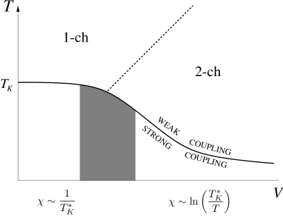
Figure 3: Schematic crossover diagram for the two-lead Kondo model. The dashed line separates the regions $V<T$ and $V>T$ corresponding to one- and two-channel scaling behavior respectively. The solid line represents the crossover from the weak- to the strong-coupling region, estimated from perturbative calculations.

If indeed $T^{*}_{K}$ is the only scale in the problem, the susceptibility and frequency-dependent conductivity in this system are expected to display the following logarithmic forms at low temperature:

$$G(\omega) \sim \frac{e^{2}}{\hbar}\ln\left[\frac{T^{*}_{K}}{\hbox{max}[|\omega-V|,T]}\right],$$ (12)

$$\chi(T,V) \sim \frac{1}{T^{*}_{K}}\ln\left[\frac{T^{*}_{K}}{T}\right].$$ (13)

If these tentative forms hold true, then the spin susceptibility must go from a finite value at low voltages to a divergent form at high voltages, suggesting the possibility of a quantum critical point separating the low and high voltage regimes of the quantum dot.

We end by adding a brief remark on the issue of decoherence. A common view is that large voltages decohere the spin fluctuations of the quantum dot, introducing a decoherence time given by $\tau^{-1}\approx(\rho J)^{2}V.$ (See, for example, eq. (43) of Wingreen:1994 and p. 387 of Kaminski:1999 .) If this decoherence is to destroy the Kondo effect, it must cut the logarithms in expressions like (2) before strong coupling is achieved. But in order for terms of the type $\ln\left(D/\mbox{max}\,(\tau^{-1},T)\right)$ to appear in the high temperature expansion, the perturbation theory would have to break down at a temperature larger than $T^{*}_{K}$, for which there is no evidence in the low-order perturbation theory. Unless such a breakdown occurs at higher orders, we conclude that $\tau^{-1}<T_{K}^{*}$.

To conclude, we have presented perturbative arguments which suggest that the two-lead Kondo model, representing a quantum dot deep in the Coulomb blockade regime, retains its strong-coupling nature even for voltages $V>T_{K}$. To reach this conclusion, we have used a perturbative calculation of the magnetic susceptibility to read off the leading renormalization behavior. We concluded that $J_{LR}$ ceases to renormalize at scales of order $V$, while $J_{L}$ and $J_{R}$ continue to renormalize, though more slowly, towards strong coupling. This suggests a picture in which the model scales to a two-channel infra-red fixed point. To test this picture, we performed a partial analysis of the stability of this point with respect to small perturbations of the form $J_{LR}$. At finite voltages, the point was found to be stable to such perturbations, although the rôle of dangerous irrelevant operators may warrant further inspection. The voltage dependence of $T_{K}^{*}$, and the associated crossover to two-channel Kondo behavior, imply that the voltage, rather than simply providing a frequency shift, qualitatively changes the structure of the model’s excitation spectrum.

We would like to thank C. Bolech, R. Aguado, D. Langreth, A. Kaminski, and L. Glazman for useful discussions. We note that related ideas are being pursued independently by Carlos Bolech and Natan Andrei using a Keldysh effective action. This work was supported by DOE grant DE-FG02-00ER45790 (PC), NSF grant DMR 99-76665 (OP), EPSRC fellowship GR/M70476 (CH), and the Lindemann Trust Foundation (CH).

References

- (1) M. Kastner, Physics Today 46, 24 (1993).
- (2) U. Meirav and E. B. Foxman, Semicond. Sci. and Tech. 11, 255 (1996).
- (3) R. C. Ashoori, Nature 379, 413 (1996).
- (4) T. K. Ng and P. A. Lee, Phys. Rev. Lett. 61, 1768 (1988).
- (5) L. I. Glazman and M. E. Raikh, Pis’ma Zh. Eksp. Teor. Fiz. 47, 378 (1988) [JETP Letters 47, 452 (1988)].
- (6) Y. Meir and N. S. Wingreen, Phys. Rev. Lett. 68, 2512 (1992).
- (7) Y. Meir, N. S. Wingreen, and P. A. Lee, Phys. Rev. Lett. 70, 2601 (1993).
- (8) N. Wingreen and Y. Meir, Phys. Rev. B49, 11040 (1994).
- (9) J. König, J. Schmid, H. Schoeller, and G. Schön, Phys. Rev. B54, 16820 (1996).
- (10) D. Goldhaber-Gordon et al., Nature 391, 156 (1998).
- (11) S. M. Cronenwett, T. H. Oosterkamp, and L. P. Kouwenhoven, Science 281, 540 (1998).
- (12) J. Schmid, J. Weis, K. Eberl, and K. von Klitzing, Physica B258, 182 (1998).
- (13) W. G. van der Wiel et al., Science 289, 2105 (2000).
- (14) A. Kaminski, Yu. V. Nazarov, and L. I. Glazman, cond-mat/0003353.
- (15) M. Plihal, D. C. Langreth, P. Nordlander, Phys. Rev. B61, R13341 (2000).
- (16) A. Schiller and S. Hershfield, Phys. Rev. B58, 14978 (1998).
- (17) Y. Avishai and Y. Goldin, Phys. Rev. Lett. 81, 5394 (1998).
- (18) J. R. Schrieffer and P. A. Wolff, Phys. Rev. 149, 491 (1966).
- (19) A. Kaminski, Yu. V. Nazarov, and L. I. Glazman, Phys. Rev. Lett. 83, 384 (1999).
- (20) For a review of the Keldysh method, see for example J. Rammer and H. Smith, Rev. Mod. Phys. 58, 323 (1986). Since this method involves only real-time evolution, it is necessary to couple the spin to a bath to allow relaxation of its magnetization at long times. We achieve this by endowing the Majorana fermions with a fictitious dispersion, which is removed at the end of the calculation. This may be shown to reproduce the known equilibrium results in the limit .
- (21) A third order analysis in the coupling constants restores the prefactor to this expression.
- (22) H. Schoeller and J. König, Phys. Rev. Lett. 84, 3686 (2000); H. Schoeller, cond-mat/9909400.
- (23) P. W. Anderson, Comm. Solid St. Phys. 5, 72 (1973).
- (24) X.-G. Wen, cond-mat/9812431.
- (25) I. Affleck and A. W. W. Ludwig, Phys. Rev. B48, 7297 (1993); A. M. Sengupta and A. Georges, Phys. Rev. B49, 10020 (1994).