Random matrix theory for systems with an approximate symmetry
and widths of acoustic resonances in thin chaotic plates

Abstract

We discuss a random matrix model of systems with an approximate symmetry and present the spectral fluctuation statistics and eigenvector characteristics for the model. An acoustic resonator like, e.g., an aluminium plate may have an approximate symmetry. We have measured the frequency spectrum and the widths for acoustic resonances in thin aluminium plates, cut in the shape of the so-called three-leaf clover. Due to the mirror symmetry through the middle plane of the plate, each resonance of the plate belongs to one of two mode classes and we show how to separate the modes into these two classes using their measured widths. We compare the spectral statistics of each mode class with results for the Gaussian orthogonal ensemble. By cutting a slit of increasing depth on one face of the plate, we gradually break the mirror symmetry and study the transition that takes place as the two classes are mixed. Presenting the spectral fluctuation statistics and the distribution of widths for the resonances, we find that this transition is well described by the random matrix model.
PACS numbers: 05.45.Mt, 62.30.+d

I Introduction

Random matrix theory has been used with success in a variety of physical systems for the description of certain generic features of spectral correlators which are determined by the underlying symmetries of the Hamiltonian [1]. In Sec. II of this paper we discuss a random matrix model of systems with an approximate symmetry. A problem like this is found, e.g., in nuclear physics where isospin symmetry, characteristic of the strong interactions, is only approximate due to Coulomb effects [2]. Isospin mixing was analysed by Guhr and Weidenmüller in 1990 using a random matrix approach [3]. They used a random matrix model to describe experimental data and to estimate the average symmetry-breaking matrix element, i.e., the average Coulomb matrix element. The random matrix model discussed here differs from the one considered in [3], and we comment on this difference. In addition to the spectral fluctuation statistics for the model we consider a measure of the asymmetry of the eigenvectors and describe it using simple analytical arguments.

In Sec. III we present two experimental studies of acoustic resonances in thin aluminium plates. The plates have the shape of the so-called three-leaf clover, see Sec. III B. Frequency spectra of acoustic resonators were first compared with random matrix results by Weaver in 1989 [4]. Further experimental studies of the fluctuation properties of acoustic resonance spectra in blocks of aluminium and quartz were made by Ellegaard and coworkers [5, 6]. In Ref. [7] the level spacing distribution measured in [6] was compared with the random matrix model of [3]. In this paper we focus on acoustic plates which in many respects are simpler than the three-dimensional resonators mentioned before. Acoustic resonances in plates were investigated by Bertelsen et al. [8]. We present a short review of the theory of acoustic waves in thin isotropic plates and discuss the characteristics of the different types of resonances. We find experimentally that modes can be separated into two different classes which each have a characteristic dependence of their widths on the damping by the air surrounding the plate. One class of modes has widths which are almost independent of the air-pressure, and the other class has widths with a strong dependence on the air-pressure. We argue that these modes are in-plane and flexural modes, respectively. In the first experiment, we measure the spectral fluctuation statistics for both mode types individually and compare with well-known results for the Gaussian orthogonal ensemble (GOE). Then, in a second experiment, we mix the two mode classes by gradually cutting a slit on one face of the plate. We thus observe the transition from two separate classes of modes to one class of modes. This transition is studied by comparing the data to the random matrix model for systems with an approximate symmetry for both the spectral fluctuation statistics and the width distribution. The latter is described using eigenvector information from the model.

II Random Matrices and Approximate Symmetries

A The random matrix model

Let $H$ be a random real symmetric $N\times N$ matrix with the following block-structure:

$$H\ =\ \left(\begin{array}[]{cc}D_{A}+A&0\\ 0&D_{B}+B\end{array}\right)\ +\ g\ \left(\begin{array}[]{cc}0&C\\ C^{T}&0\end{array}\right)\ ,$$ (1)

where $D_{A}$ and $A$ are random $N_{1}\times N_{1}$ matrices, and $D_{B}$ and $B$ are random $N_{2}\times N_{2}$ matrices. The random matrix $C$ is $N_{1}\times N_{2}$, and the coupling strength, $g$, is a real parameter. Note that $N\equiv N_{1}+N_{2}$. The elements of the diagonal matrices $D_{A}$ and $D_{B}$ are drawn uniformly on the interval $[-0.5,0.5]$ and ordered in increasing order for each block. This choice of probability distribution leads to level spectra for $D_{A}$ and $D_{B}$ which, except for small end-point corrections, are described by the Poisson statistics appropriate for a sequence of uncorrelated energy levels. The elements of $A$, $B$, and $C$ are Gaussian distributed with zero mean. The variance, $\sigma^{2}$, of the distribution of the diagonal elements of $A$ and $B$ scales as $1/N^{2}$. The variance of the distribution of the off-diagonal elements of the matrices $A$ and $B$ and the elements of $C$ is set to half the value of $\sigma^{2}$.

The diagonal contributions $D_{A}$ and $D_{B}$ in $H$ are intended to mimic the effects of the kinetic energy operator, and the Gaussian distributed elements of $A$ and $B$ simulate “interactions” due to boundary conditions. Since the elements of $D_{A}$ and $D_{B}$ are “sufficiently” small compared with the Gaussian distributed elements, the short-range spectral fluctuation statistics are identical to the statistics obtained for two superimposed GOE spectra (2 GOE) when $g=0$ and to GOE statistics when $g=1$. (See Sec. II B for a more detailed discussion of the spectral fluctuation statistics.) The average distance between neighbouring levels scales as $1/N$ because of the presence of the diagonal matrix elements. With a finite value of $g$ both the root mean square (RMS) symmetry-preserving matrix element and the RMS symmetry-breaking matrix element also scale like $1/N$, and the transition from 2 GOE statistics to GOE statistics takes place as a function of $g$ independent of the value of $N$.

This is not the case if the kinetic energy terms are not present as in a random matrix model, like the one used in Refs. [3, 7], with two GOE-like diagonal blocks coupled by Gaussian-distributed matrix elements. For such a model the ratio between the RMS symmetry-breaking matrix element and the average distance between neighbouring levels for the unperturbed problem scales like $g\sqrt{N}$. The transition from 2 GOE to GOE spectral fluctuation statistics takes place as a function of this ratio. If $g$ is independent of $N$, it follows that the ratio scales like $\sqrt{N}$, and in particular that it goes to infinity in the large-$N$ limit for any finite value of $g$. To observe a smooth transition from 2 GOE statistics to GOE statistics independent of $N$, it is thus necessary that the ratio between the RMS symmetry-breaking matrix element and the RMS symmetry-preserving matrix element scales like $1/\sqrt{N}$ in a random matrix model without kinetic energy terms.

B Spectral fluctuation statistics

To describe the short-range spectral fluctuation statistics we consider the standard level spacing distribution, and as a measure of the long-range spectral fluctuation statistics we choose to look at the $\Delta_{3}$-statistic [9]. Numerical calculations of the level spacing distribution and the $\Delta_{3}$-statistic for $N_{2}=2N_{1}=200$ with $\sigma^{2}=16/N^{2}$ are shown in Figs. 1 and 2 together with the exact results for the GOE and two superimposed GOE spectra with fractional densities 1/3 and 2/3, respectively. The ensembles in the simulations consisted of 500 matrices, and 150 eigenvalues from the “middle” of the spectrum for each matrix were considered. Figures 1(a) and 1(d) show that the level spacing distribution for the random matrix model is identical to the 2 GOE result when $g=0$ and to the GOE result when $g=1$. Similarly Fig. 2 shows that this is also the case for $\Delta_{3}(L)$ for $L\leq 20$. It is clear from Fig. 1 that the level spacing distribution looks very much like the level spacing distribution for the GOE even when $g=0.1$. It is well known that $\Delta_{3}(L)$ for a model with diagonal terms like $D_{A}$ and $D_{B}$ deviates from the corresponding GOE result for large values of $L$ [10]. The value of $L$ where this transition to more Poisson-like behaviour sets in is referred to as the Thouless energy. For $g=1$ and $\sigma^{2}=16/N^{2}$ we find a Thouless energy of about 35. A different choice of the variance, $\sigma^{2}$, leads to a picture for the spectral fluctuation statistics similar to the one shown on Figs. 1 and 2 as long as $L$ is less than the Thouless energy.

C Eigenvector information

As a measure of the asymmetry of the eigenvectors of $H$ we define a quantity, $a$, which we denote the asymmetry number. Consider a $N=N_{1}+N_{2}$ dimensional vector $(v_{1},v_{2},...,v_{N})$ of unit length, and let $a$ be defined by

$$a\ \equiv\ \sum_{i=1}^{N_{1}}v_{i}^{2}-\sum_{i=N_{1}+1}^{N}v_{i}^{2}\ .$$ (2)

For two decoupled systems described by the subspaces spanned by the first $N_{1}$ and the last $N_{2}$ basis vectors, respectively, the distribution $P_{A}(a)$ has a $\delta$-function peak at $a=-1$ and one at $a=1$. For the GOE it has a single peak at $a=(N_{1}-N_{2})/N$. These features are obvious in Fig. 3, which shows $P_{A}$ calculated numerically for the ensembles considered in Sec. II B. Notice that the smaller of the two peaks present when $g=0$ has almost vanished when $g=0.1$, whereas the strength of the largest peak is reduced to half its original value.

Imagine that two uncoupled classes of resonances have width distributions $P_{F}$ and $P_{I}$, respectively. The width distribution of all the resonances, $P(\Gamma)$, is the sum of $P_{F}$ and $P_{I}$ when the two classes are uncoupled. The width distribution, $P(\Gamma)$, changes if the two classes are coupled, and in our random matrix approach we model $P(\Gamma)$ using the asymmetry distribution:

$$P(\Gamma) = \int_{0}^{1}\textrm{d}x\int_{-\infty}^{\infty}\textrm{d}\Gamma_{F}\int_{-\infty}^{\infty}\textrm{d}\Gamma_{I}$$ (4)

$$\times\ \delta(\Gamma-x\Gamma_{F}-[1-x]\Gamma_{I})\ 2P_{A}(1-2x)P_{F}(\Gamma_{F})P_{I}(\Gamma_{I})$$

$$= \int_{0}^{1}\textrm{d}x\frac{2P_{A}(1-2x)}{1-x}\int_{-\infty}^{\infty}\textrm{d}\Gamma_{F}P_{F}(\Gamma_{F})P_{I}\left(\frac{\Gamma-x\Gamma_{F}}{1-x}\right)\ .$$ (5)

Notice that the integral reduces to the weighted sum of $P_{F}$ and $P_{I}$ if $P_{A}$ is the sum of two $\delta$-functions as in the case $g=0$ shown in Fig. 3(a), and that $P$ is expressed in terms of $P_{A}$ if $P_{F}$ and $P_{I}$ are $\delta$-functions.

We now consider the case $N_{1}=N_{2}$ and describe the characteristic properties of the asymmetry distribution using a simple analytical model and arguments from perturbation theory. Figure 4 shows numerical calculations of the distribution of the asymmetry numbers for $N_{1}=N_{2}=150$ for three values of $g$. We considered ensembles of 500 random matrices, and, as in the numerical simulations described in Sec. II B, we focused on the 150 eigenvalues in the “middle” of the spectrum. The distribution $P_{A}(a)$ increases linearly as a function of $g$ close to $a=0$ as shown in Fig. 4(d).

The small fraction of the eigenvectors for which the asymmetry number is close to zero are most likely superpositions of an eigenvector of $D_{A}+A$ and an eigenvector of $D_{B}+B$ with eigenvalues lying close in the unperturbed spectrum where $g=0$. Let the unperturbed spacing between the two eigenvalues be denoted $\Delta$ and consider the matrix which connect the two states when the symmetry-breaking perturbation is introduced:

$$H_{c}=\left(\begin{array}[]{cc}0&c\\ c&\Delta\end{array}\right)\ .$$ (6)

The distribution, $P_{C}$, of the matrix elements, $c$, is Gaussian with zero mean and variance $(g\sigma)^{2}/2$. In the numerical simulation shown in Fig. 4 the eigenvectors come from the “middle” of the eigenvalue spectrum where the level density is almost constant, and we thus assume that the level density for each diagonal block is equal to a constant which we denote $R_{1}$. In this case the spacing, $\Delta$, comes from the distribution

$$P_{\Delta}(\Delta)=\frac{1}{\sqrt{2\pi}\Delta_{0}}\exp\left(\ -\frac{\Delta^{2}}{2\Delta_{0}^{2}}\ \right)\ ,$$ (7)

where the variance $\Delta_{0}^{2}=1/(2\pi R_{1}^{2})$. In the two-dimensional approximation the eigenvectors have the asymmetry numbers

$$a=\pm\frac{1}{\sqrt{1+4c^{2}/\Delta^{2}}}\ ,$$ (8)

and thus the distribution of the asymmetry numbers becomes

$$P_{A}(a) = \frac{1}{2}\int_{-\infty}^{\infty}\textrm{d}c\int_{-\infty}^{\infty}\textrm{d}\Delta\ P_{C}(c)P_{\Delta}(\Delta)$$ (10)

$$\times\left[\delta\left(a-\frac{1}{\sqrt{1+4c^{2}/\Delta^{2}}}\right)+\delta\left(a+\frac{1}{\sqrt{1+4c^{2}/\Delta^{2}}}\right)\right]\$$

$$= \frac{\sqrt{2}\sigma g}{\pi\Delta_{0}\sqrt{1-a^{2}}[1-a^{2}+(\sqrt{2}a\sigma g/\Delta_{0})^{2}]}\ .$$ (11)

When $a=0$ the expression reduces to

$$P_{A}(0)=\frac{2\sigma R_{1}}{\sqrt{\pi}}g\ ,$$ (12)

which is in perfect agreement with the numerical simulation shown in Fig. 4 for which $\sigma=4/300$ and $R_{1}=140$.

The majority of the eigenvectors, which have values of $|a|\approx 1$, can be described using perturbation theory. The shift in the position of the peak of the distribution away from $a=1$ is to first order proportional to $g^{2}$, since the average correction to a given state from a state from the other block is proportional to $g$.

III The Acoustic Experiment

A Acoustic resonances in thin plates

In a homogeneous and isotropic three-dimensional medium, sound waves obey the elastomechanical wave equation for the vectorial displacement field ${\bf u}$:

$$\rho{\partial^{2}{\bf u}\over\partial t^{2}}=(\lambda+\mu)\nabla(\nabla\cdot{\bf u})+\mu\nabla^{2}{\bf u}\;,$$ (13)

where $\lambda$ and $\mu$ are the Lamé coefficients, $\rho$ is the density, and we have assumed no external forces. Equation (13) allows for two types of wave motion: longitudinal and transverse. (In the literature the transverse modes have names like shear or secondary, and the longitudinal modes are often called pressure or primary.) Longitudinal waves always travel faster than transverse waves. For aluminium, which we consider in this paper, the difference is approximately a factor of 2. In the bulk, the two types of waves propagate independently. However, upon reflection at a boundary, mode conversion takes place: an incident wave that is purely longitudinal or transverse will, in general, give rise to two reflected waves, one longitudinal and one transverse. Moreover, their angles of reflection will be different due to their different velocities, as dictated by Snell’s law.

We now briefly present some facts about elastic waves in thin infinite plates, see, e.g., [11] and the recent studies in Ref. [8, 12]. Three types of modes exist in an infinite isotropic plate, when considered at frequencies below the first critical frequency, i.e., when one half of a transverse wavelength is larger than the thickness of the plate. The flexural modes have displacement mainly normal to the plane of the plate, but they also have a small in-plane component. These modes are anti-symmetric with respect to reflection through the middle plane of the plate. (In the literature the flexural modes are sometimes called bending modes.) The in-plane modes are symmetric with respect to reflection through the middle plane of the plate and consist of two mode types. The in-plane transverse modes have displacement exactly in the plane of the plate, and the in-plane longitudinal modes have displacement mainly in the plane of the plate, but they also have a small out-of-plane component.

Now consider a finite plate. As mentioned above, the boundaries introduce mode conversion. For a finite plate there is thus the possibility of a coupling between the different mode classes. In Ref. [8] it was concluded, first, that the flexural modes are uncoupled from the in-plane modes and, second, that the in-plane longitudinal modes couple to the in-plane transverse modes. The densities of flexural modes and in-plane modes were calculated theoretically and found to be of the same order [8]. These results explain the spectral fluctuation statistics measured in Ref. [8] where resonances, i.e., both flexural and in-plane modes, of a quarter of a thin Sinai stadium plate were investigated. In Sec. III C we explain how to separate the flexural and in-plane modes experimentally using their measured widths. This technique allows us to measure the number of modes of the two types separately and to compare these numbers to the theoretical predictions of Ref. [8]. It also enables us to study the spectral statistics and the width distributions for the two classes of modes independently and to find out if the flexural modes are in fact uncoupled from the other modes.

B Acoustic systems and experimental technique

For the experiments, we use two aluminium plates of different thickness cut in the shape of the three-leaf clover shown in Fig. 5. This billiard, which was first considered in Ref. [13], was chosen because it is known to be classically chaotic and, when $R\geq r$, it has no continuous families of periodic orbits [14]. Thus, we have chosen $r=70$ mm and $R=80$ mm. The area of the plates was $8250\pm 100$ mm², and the circumference was $390\pm 3$ mm. The plates were $1.5$ mm and $2$ mm thick.

The choices of $r$ and $R$ and the thickness are important for the experiment in so far as they determine the relative densities of the two mode classes and also the total number of modes. In our case, these parameters were chosen to give many modes for the purpose of producing significant statistics while keeping the density of in-plane modes approximately equal to the density of flexural modes in the frequency range (300 kHz – 600 kHz) where our transducers are most effective.

Aluminium was chosen for the plates because it is isotropic and very easy to machine, while maintaining a high Q value; at 500 kHz the Q value measured in vacuum is around 10⁴. There are isotropic materials with much higher Q values, such as fused quartz. However, fused quartz is more difficult to machine and thus not suitable for the symmetry-breaking experiment, where one must remove material from the plate many times in a controlled way.

The elastic constants for the two plates cannot be found in standard tables of material properties, since they are not pure aluminium but a special alloy. However, the elastic constants for this alloy were determined by experiment in Ref. [15]. We shall use the values from Ref. [15] for Young’s modulus $E=$70 $\pm$ 1 GPa and Poisson’s ratio $\nu=$0.330 $\pm$ 0.005. The density is 2.698 g/cm³ [16]. The corresponding bulk sound velocities are 3123 m/s for transverse waves and 6200 m/s for longitudinal waves.

The experimental setup is in many ways the same as that used for previous experiments as reported in [17]. We use an HP 3589A spectrum/network analyser to measure transmission spectra of acoustic resonators via piezoelectric transducers. The plate rests horizontally, supported by three gramophone diamond styli. This ensures a very small contact area between the plate and the rest of the world, thus making the vibrations of the plate as close to free as possible. The diamond styli are glued to cylindrical piezo ceramics that are polarised along the symmetry axis (z-axis). One such combination functions as transmitter, the two others as receivers.

One may wonder if our experimental technique can really measure all modes. In particular, one could question if the in-plane modes, for which the displacement is mainly (or exactly) in the plane of the plate, are detected by our transducers. This question was answered in Ref. [8], where the same experimental technique is used. The authors find that all modes are detected. To understand this, one can imagine what happens microscopically when strain is passed from the plate to the piezoelectric component through the diamond stylus. Obviously, there can be no slip between the tip of the stylus and the plate. If there were indeed slip, there would also be friction. The diamond would then quickly drill a hole in the plate, and this is not observed in the experiments. In fact, after many days of oscillations at frequencies of several hundred kHz, the plate is completely intact. Since the base of the diamond stylus is fixed to the piezo electric component, the diamond stylus undergoes a wiggling motion which deforms the piezo electric component in a complicated way, including compression along the z-axis.

In both of the experiments the temperature was room temperature, i.e., it was not kept constant but could fluctuate by a few degrees. Obviously, the temperature is important in these measurements, since both the size of the plate and the elastic constants depend on the temperature, and changes in these parameters affect the eigenfrequencies. However, for aluminium thermal expansion is the dominant effect, and to first order eigenfrequencies shift locally by the same amount. Since we are not interested in single eigenfrequencies but only in differences between them, this shift has no influence on our results.

The plate is placed in a vacuum chamber, which allows control of the pressure of the air surrounding the plate. At pressures lower than $10^{-2}$ Torr air damping is insignificant compared to intrinsic losses and losses to the supports. Therefore, we shall refer to such low pressure as “vacuum”. When the pressure is increased, the flexural modes, that have large out-of-plane oscillations, are strongly affected, since the plate then functions like a loudspeaker generating sound waves in the air. As a result, the amplitudes of the flexural modes decrease with increasing pressure, and the widths of the resonance peaks increase. This is demonstrated in Fig. 6, which shows a section of the transmission spectrum measured for the three-leaf clover in vacuum, at a pressure of 0.5 atm, and at atmospheric pressure. Note that one can label most of the modes into flexural and in-plane by eye.

C The separation experiment

The first experiment was designed to separate the modes into flexural and in-plane types so that the spectral statistics could be studied separately for each class. To get a statistically significant result, many eigenfrequencies are needed, and it is crucial to find all the levels so that the results are free from missing level effects. For this reason we performed the following measurement sequence. The acoustic transmission spectrum for the plate of thickness 2 mm was measured in the range 300 kHz – 540 kHz. The measurement was carried out first in vacuum, then at a pressure of 0.5 atm, and finally at 1 atm, see Fig. 6. In each case, the measurement was performed twice, using two independent receivers. This procedure gave 6 resonance spectra. Then, the system was subject to a perturbation, when a mass of 14 mg, corresponding to 314 ppm, was removed from one face of the plate using a piece of fine sand paper. After this, the above procedure was repeated, giving another 6 resonance spectra. Then, in the same way, another perturbation was made, this time removing 43 mg of material, corresponding to 965 ppm. Again, the measurement sequence was carried out, giving a total of 18 resonance spectra. The perturbations done to the system are small enough that it is possible to follow every resonance peak through all 18 spectra, but large enough that near-degeneracies in one set of spectra are destroyed by the perturbations, giving well-resolved peaks in the next set of spectra. This technique allows us to find all resonances. There are no missing levels.

We would like to establish a simple and reliable criterion that permits us to separate the spectrum into flexural and in-plane modes. To this end, each resonance peak is fitted using the so-called “skew Lorentzian” approach [18]. This fit yields a number of parameters of which only the resonance frequency and the width, $\Gamma$, are of interest. In Fig. 7 we show the distribution of widths obtained from this fitting procedure for increasing values of the air pressure. It is evident that the widths of one group of modes increases with increasing pressure while the widths of the remaining modes is largely unaffected. We interpret these groups as flexural and in-plane modes, respectively. However, even at atmospheric pressure, it is not possible to separate the modes on the basis of resonance width alone.

Since the width distribution does not allow us to separate the flexural modes from the in-plane modes with certainty, we must find a more reliable criterion. Therefore, we consider the individual resonance widths as function of pressure, see Fig. 8.

The curves for the two resonances in Fig. 8 are typical for the measured modes and show that the curves are well approximated by straight lines. Consequently, it makes sense to label them by the slope of the best straight line fit. We then consider the distribution of these slopes, see Fig. 9. The distribution has two well-separated peaks. Large slopes correspond to flexural modes; small slopes correspond to in-plane modes. Based on this information, we choose the “separation” slope to be 11 Hz/atm.

In the range 300 kHz to 540 kHz we find 1537 levels for the 2 mm plate, of which 781 are flexural and 756 are in-plane, judging from the separation criterion discussed above. Reference [8] presents an expansion of the exact dispersion relations for an infinite isotropic plate and also gives the corresponding expansion for the number of modes, i.e., the staircase function, for a finite, thin plate. Using this theoretical expansion, we expect $782$ flexural modes and $753$ in-plane modes. This is in perfect agreement with the measured numbers, given the uncertainty in the elastic constants of the aluminium alloy and in the dimensions of the plate.

Since we can identify the character of individual modes, it is possible to consider the level spacing distribution and the $\Delta_{3}$-statistic separately for each of the two classes. Figures 10 and 11 show the level spacing distribution and the $\Delta_{3}$-statistic for each of the two mode classes compared with the GOE statistics. We find that both the level spacing distribution and the $\Delta_{3}$-statistic for the flexural modes agree with the GOE statistics. This result confirms numerical calculations by Bogomolny and Hugues showing that the flexural modes of a chaotic billiard have GOE fluctuation statistics, see Ref. [12]. The $\Delta_{3}$-statistic for the in-plane modes lies above the GOE curve. This is a bit surprising, because mode conversion is expected to be a strong effect, see, e.g. Ref. [19], which should guarantee that all in-plane modes are strongly coupled and obey GOE statistics. We note that the deviation from the GOE curve seen in the $\Delta_{3}$-statistic does not appear in the spacing distribution; the spacing distribution for the in-plane modes looks much like the spacing distribution for the GOE. The same feature is seen for the random matrix model for systems with an approximate symmetry, see the results for $g=0.2$ on Figs. 1(c) and 2. If we think of mode conversion as a mechanism that breaks the longitudinal-transverse “symmetry” for in-plane modes, our results could indicate that this symmetry is not completely broken.

An issue to consider in this context is the value of the wavelength, $\lambda$, compared to the size, $l$, of the system. The ratio $l/\lambda$ is a measure of how “semiclassical” our system is. Roughly, $l=100$ mm. Random matrix results are only expected to apply when $l/\lambda\gg 1$. For flexural modes, the typical wavelength is 5 mm, so $l/\lambda=20$. For travelling in-plane waves, the typical transverse wavelength is 7 mm and the typical longitudinal wavelength is 13 mm. Roughly, this leads to $l/\lambda=10$. Thus, in our experiments we have the two length scales separated by at least an order of magnitude. Nevertheless, the factor of 2 between $l/\lambda$ for flexural and in-plane modes shows that the flexural modes are more “semiclassical” than the in-plane modes, which is another possible explanation for the slight difference observed in the fluctuation properties.

We emphasise that the main results of this section are, first, that the flexural and the in-plane modes can be separated and, second, that each of the two mode classes behave as one class of strongly-coupled modes. The fact that the $\Delta_{3}$-statistic lies slightly above the GOE curve for the in-plane modes is a small correction to this picture. In the following section, we regard the in-plane modes as one class of strongly-coupled modes.

D The symmetry-breaking experiment

The second experiment was designed for a detailed study of the transition from two independent mode classes to one mode class. The transition takes place as the mirror-symmetry through the middle plane of the plate is broken. For this experiment, we used the three-leaf clover plate of thickness 1.5 mm and gradually cut a slit on one side of the plate, as shown in Fig. 12.

For the cutting of the slit in the plate we used a computer-controlled milling machine and chose steps in the thickness of 1/40 mm. In our case, this amounted to about 18 mg of material for each increment of the depth of the slit. The mass of the intact plate was 32.8870 g. First, the frequency spectrum was measured for the intact plate in vacuum and at atmospheric pressure. The procedure of cutting and measuring the frequency spectrum at atmospheric pressure was then repeated 9 times. In all measurements the frequency range was 456 kHz – 533 kHz and only one receiver was used. The justification for using just one receiver for this experiment is as follows: Removal of material from the plate corresponds to a small perturbation. One can therefore easily follow each resonance peak through the entire scenario, and although a resonance peak can sometimes disappear in one spectrum because the receiver is accidentally placed on a nodal line, it always reappears in subsequent spectra. Thus, the results of this symmetry-breaking experiment are protected against missing level effects.

As in the previous experiment, the resonance peaks are fitted and we calculate the distribution of widths, focusing first on the intact plate. In the plot for atmospheric pressure, the modes are separated into two classes: those that have widths smaller than 22 Hz and those that have widths larger than 22 Hz, see Fig. 15. This sets the criterion for separation of the flexural modes from the in-plane modes. We note that for the 1.5 mm plate it is possible to perform the separation purely on the basis of the widths measured at atmospheric pressure. This was not the case for the 2 mm plate.

In general, we expect that the widths of the flexural modes at some value of the pressure will depend on many parameters. Among these, the thickness of the plate and the typical wavelength play important roles. However, comparing our two experiments, all of the parameters are the same except for the thickness. The average width for the in-plane modes is about the same in the two cases. At a pressure of 1 atm, the mean width for the flexural modes for the 2 mm plate is around 35 Hz and for the 1.5 mm plate the mean width is 42 Hz. This indicates that damping from the air is larger for thinner plates.

We consider first the plate before any material has been removed and find 600 levels in the frequency range 456 kHz - 533 kHz. According to our separation rule, this time based solely on the width distribution measured at atmospheric pressure, 310 modes are flexural and 290 are in-plane. Using again the expansion for the number of modes given in Ref. [8], there should be 311 flexural modes and 285 in-plane modes, in perfect agreement with our results. As in Sec. III C we have obtained the level spacing distribution and the $\Delta_{3}$-statistic for the two mode classes separately. We find the same spectral statistics for the 1.5 mm plate as for the 2 mm plate.

Figures 13 and 14 show the level spacing distributions and the $\Delta_{3}$-statistics for all the modes for increasing depth of the symmetry-breaking slit. The experimental data are fitted with results for the random matrix model of Sec. II. We have used $N_{1}=N_{2}=150$ and $\sigma^{2}=64/N^{2}$. Table I summarises the results for the theoretical fits to the spectral statistics for the symmetry breaking experiment. The spectral statistics are well described by the model, and the best fits to the level spacing distribution and to the $\Delta_{3}$-statistic yield consistent values for the coupling strength $g$.

In Fig. 15 the measured width distributions are compared with the distributions calculated numerically using Eq. (4). To model the width distribution $P(\Gamma)$ for all modes, we use the asymmetry distribution for the eigenvectors and assume that the in-plane modes and the flexural modes have Gaussian width distributions $P_{I}$ and $P_{F}$. For each of the different cases we fix the value of the coupling strength, $g$, to the value obtained from the spectral statistics. For the intact plate, see Fig. 15(a), we fitted the width distribution by minimising $\chi^{2}$, and found the mean values $\Gamma_{I}^{0}$ = 12.2 Hz and $\Gamma_{F}^{0}$ = 42.0 Hz, and the standard deviations $\sigma_{I}$ = 2.8 Hz and $\sigma_{F}$ = 5.8 Hz. The mean values for the fit agree with the measured average width of 27.1 Hz, see Tab. I. The average width depends on the slit depth as shown in Tab. I, and increases, e.g., by 2.1 Hz when the cut increases from 0 mg to 37.4 mg. To take effects like this into account we have fitted the width distributions by varying the four parameters $\Gamma_{I}^{0}$, $\Gamma_{F}^{0}$, $\sigma_{I}$, and $\sigma_{F}$. The only parameter which changed significantly from case to case was the average width of the flexural resonances, $\Gamma_{F}^{0}$. This seems reasonable since we expect that the modes with large out-of-plane components are damped most by surface perturbations like the cut. For the width distributions shown in Fig. 15(b), (c), and (d) we therefore held $\Gamma_{I}^{0}$, $\sigma_{I}$, and $\sigma_{F}$ fixed, whereas $\Gamma_{F}^{0}$ was varied so that the average width equalled the measured average shown in Tab. I. The overall features of the width distribution as function of slit depth are described by the random matrix model. As the slit depth increases, the strength of the width distribution between the two peaks increases while the strength of the peaks decreases. Notice that the value of $P(\Gamma)$ around $\Gamma=27.5$ Hz increases linearly with $g$ in agreement with Eq. (8).

IV Discussion and Conclusions

We have presented experimental results for acoustic resonances in two thin aluminium plates of three-leaf clover shape. For both plates we found that the measured number of flexural and in-plane resonances were in very good agreement with the theoretical Weyl formula. The two classes of modes were separated using their width or the dependence of the width on the pressure of the air surrounding the plate. The spectral statistics for the flexural modes were in perfect agreement with the GOE result in both cases whereas the spectra of the in-plane modes seemed to be slightly less rigid than the GOE.

The random matrix model of systems with an approximate symmetry modelled the experimental data on the spectral statistics and wave function information from the mixing experiment well. Both the level spacing distribution, the $\Delta_{3}$-statistic, and the distribution of widths were fitted consistently by the numerical random matrix results. The qualitative changes in the width distribution as the depth of the cut was increased could thus be ascribed to the complex mixed nature of the acoustic wave functions.

The successful description of the statistics of the frequency spectrum and the widths of the thin acoustic plates may be extended to include other features. The presence of both a kinetic energy term and an interaction term in the random matrix model is natural not only in the modelling of the mixing process but also to describe the Thouless energy of acoustic resonators due to the localisation of wave functions. In this way the model represents an extension of the simplest random matrix models, like the GOE, to include several important features present in real physical systems.

TABLE I.: The first column shows the size of the cut and the fourth column the average width. The second and third column show estimates of $g$ obtained by fitting the level spacing distribution and the $\Delta_{3}$-statistic, respectively.

Cut [mg]	$g$ from ls	$g$ from $\Delta_{3}$	Mean width [Hz]
0.0	0.01	0.00	27.1
10.3	0.02	0.00	27.9
23.1	0.02	0.005	28.6
37.4	0.02	0.02	29.2
55.7	0.05	0.04	29.1
71.3	0.055	0.055	29.7
92.5	0.06	0.05	30.0
108.5	0.06	0.06	30.8
128.8	0.09	0.08	30.3
146.1	0.06	0.07	29.9

FIG. 1.: The level spacing distribution for different values of $g$. The two diagonal blocks are uncoupled when $g=0$, and when $g=1$ all the basis states are coupled.

FIG. 2.: The $\Delta_{3}$-statistics for different values of $g$. The numerical simulations for $g=0$ and $g=1$ agree with the 2 GOE and the GOE result, respectively.

FIG. 3.: The asymmetry distribution $P_{A}$ for the eigenvectors. When $g=0$ each eigenvector belongs to one of the two parts of the vector space. As $g$ increases the eigenvectors get components in both of the two parts of the vector space.

FIG. 4.: The asymmetry distribution $P_{A}(a)$ obtained numerically for random matrix ensembles with $N_{1}=N_{2}$. The value $P_{A}(0)$ grows linearly with $g$, see the blow-up on (d), as predicted in the simple analytical model of the eigenvector mixing, see Eq. (12).

FIG. 5.: Sketch of the three-leaf clover (not to scale). (a) The construction of the three-leaf clover (thick solid line) with mirror symmetries indicated by dashed lines. The geometry is defined by the two radii, $r$ and $R$. (b) The plates used in the experiments were one sixth of the three-leaf clover.

FIG. 6.: A segment of the resonance spectrum for the 2 mm thick three-leaf clover at three different pressures: vacuum, 0.5 atm, and 1 atm. Most resonances are easily recognised to be either in-plane (I) or flexural (F).

FIG. 7.: The distribution of widths for the acoustic resonances for the three-leaf clover plate of thickness 2 mm, at the same values of the air-pressure as in Fig. 6. One class of modes (in-plane) have widths which are almost independent of the pressure and the widths for the other class of modes (flexural) increase with increasing pressure.

FIG. 8.: The width of a flexural mode and an in-plane mode for the three-leaf clover as function of the pressure of the air in the vacuum chamber. Six curves appear for each resonance peak, because six different measurements were made for each of the pressure values: vacuum, 0.5 atm, and 1 atm.

FIG. 9.: The distribution of slopes $\textrm{d}\Gamma/\textrm{d}p$ has two well-separated peaks, which makes it possible to separate the flexural and in-plane modes. We choose a “separation” slope of 11 Hz/atm. A few inaccurate fits gives rise to the small number of negative slopes.

FIG. 10.: The level spacing distribution (a) and the $\Delta_{3}$-statistic (b) for the flexural modes compared with the GOE statistics. Both the level spacing distribution and the $\Delta_{3}$-statistic agree very well with the GOE results.

FIG. 11.: The level spacing distribution (a) and the $\Delta_{3}$-statistic (b) for the in-plane modes compared with the GOE statistics. The $\Delta_{3}$-statistic shows that the spectrum of the in-plane modes is slightly less rigid than the GOE.

FIG. 12.: (a) A sixth of the three-leaf clover with a 2 mm wide cut indicated (not to scale). (b) Sketch of the plate profile showing how the cut breaks the mirror-symmetry through the middle plane of the plate.

FIG. 13.: The level spacing distribution for all the modes compared to the result of the random matrix model. (a) The plate is intact. (b) A total of 37.4 mg has been removed. (c) A total of 71.3 mg has been removed. (d) A total of 128.8 mg has been removed.

FIG. 14.: The $\Delta_{3}$-statistic for all the modes is fitted by minimising the sum of the squared deviations between the data and the random matrix result. (a) The plate is intact. (b) A total of 37.4 mg has been removed. (c) A total of 71.3 mg has been removed. (d) A total of 128.8 mg has been removed.

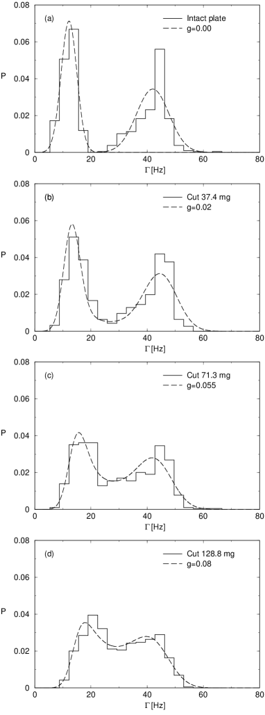
FIG. 15.: The experimental width distribution for the resonances compared to the distribution $P(\Gamma)$ obtained numerically using Eq. (4). The three plots represent data for the same slit-depths and values of $g$ as in Figs. 13 and 14. (a) The plate is intact. (b) A total of 37.4 mg has been removed. (c) A total of 71.3 mg has been removed. (d) A total of 128.8 mg has been removed.

REFERENCES

- [1] T. Guhr, A. Müller-Groeling, and H. A. Weidenmüller, Phys. Rep. 299, 189 (1998).
- [2] G. E. Mitchell, E. G. Bilpuch, P. M. Endt, and J. F. Shriner, Jr., Phys. Rev. Lett. 61, 1473 (1988).
- [3] T. Guhr and H. A. Weidenmüller, Annals of Physics 199, 412 (1990).
- [4] R. L. Weaver, J. Acoust. Soc. Am. 85, 1005 (1989).
- [5] C. Ellegaard et al., Phys. Rev. Lett. 75, 1546 (1995).
- [6] C. Ellegaard et al., Phys. Rev. Lett. 77, 4918 (1996).
- [7] D. M. Leitner, Phys. Rev. E 56, 4890 (1997).
- [8] P. Bertelsen, C. Ellegaard, and E. Hugues, Eur. Phys. J. B 15, 87 (2000).
- [9] M. L. Mehta, Random Matrices, 2nd Edition (Academic Press, New York, 1991).
- [10] T. Guhr and H. A. Weidenmüller, Annals of Physics 193, 472 (1989).
- [11] K.F. Graff, Wave Motion in Elastic Solids (Dover Publications, Inc., New York, 1975).
- [12] E. Bogomolny and E. Hugues, Phys. Rev. E 57, 5404 (1998).
- [13] C. Jarzynski, Phys. Rev. E 48, 4340 (1993).
- [14] C. Jarzynski, private communication.
- [15] P. Bertelsen, M.Sc. Thesis, CATS, Niels Bohr Institute (1997). http://www.nbi.dk/∼speciale/speciale.ps.gz.
- [16] G.W.C. Kaye and T.H. Laby, Tables of Physical and Chemical Constants, (Longman, New York, 1986)
- [17] M. Oxborrow and C. Ellegaard, in Proceedings of the 3rd International Conference on Experimental Chaos, page 251 (World Scientific, Singapore, 1996).
- [18] H. Alt et al., Nucl. Phys. A, 560, 293 (1993)
- [19] L. Couchman, E. Ott, and T. M. Antonsen, Jr., Phys. Rev. A 46, 6193 (1992).