We present exact calculations of the partition function of the $q$-state Potts model for general $q$ and temperature on strips of the square lattice of width $L_{y}=3$ vertices and arbitrary length $L_{x}$ with periodic longitudinal boundary conditions, of the following types: (i) $(FBC_{y},PBC_{x})=$ cyclic, (ii) $(FBC_{y},TPBC_{x})=$ Möbius, (iii) $(PBC_{y},PBC_{x})=$ toroidal, and (iv) $(PBC_{y},TPBC_{x})=$ Klein bottle, where $FBC$ and $(T)PBC$ refer to free and (twisted) periodic boundary conditions. Results for the $L_{y}=2$ torus and Klein bottle strips are also included. In the infinite-length limit the thermodynamic properties are discussed and some general results are given for low-temperature behavior on strips of arbitrarily great width. We determine the submanifold in the ${\mathbb{C}}^{2}$ space of $q$ and temperature where the free energy is singular for these strips. Our calculations are also used to compute certain quantities of graph-theoretic interest.

1 Introduction

The $q$-state Potts model has served as a valuable model for the study of phase transitions and critical phenomena [1, 2]. On a lattice, or, more generally, on a (connected) graph $G$, at temperature $T$, this model is defined by the partition function

$$Z(G,q,v)=\sum_{\{\sigma_{n}\}}e^{-\beta{\cal H}}$$ (1.1)

with the (zero-field) Hamiltonian

$${\cal H}=-J\sum_{\langle ij\rangle}\delta_{\sigma_{i}\sigma_{j}}$$ (1.2)

where $\sigma_{i}=1,...,q$ are the spin variables on each vertex (site) $i\in G$; $\beta=(k_{B}T)^{-1}$; and $\langle ij\rangle$ denotes pairs of adjacent vertices. The graph $G=G(V,E)$ is defined by its vertex set $V$ and its edge set $E$; we denote the number of vertices of $G$ as $n=n(G)=|V|$ and the number of edges of $G$ as $e(G)=|E|$. We use the notation

$$K=\beta J\ ,\quad a=u^{-1}=e^{K}\ ,\quad v=a-1$$ (1.3)

so that the physical ranges are (i) $a\geq 1$, i.e., $v\geq 0$ corresponding to $\infty\geq T\geq 0$ for the Potts ferromagnet, and (ii) $0\leq a\leq 1$, i.e., $-1\leq v\leq 0$, corresponding to $0\leq T\leq\infty$ for the Potts antiferromagnet. One defines the (reduced) free energy per site $f=-\beta F$, where $F$ is the actual free energy, via

$$f(\{G\},q,v)=\lim_{n\to\infty}\ln[Z(G,q,v)^{1/n}]$$ (1.4)

where we use the symbol $\{G\}$ to denote $\lim_{n\to\infty}G$ for a given family of graphs. In the present context, this $n\to\infty$ limit corresponds to the limit of infinite length for a strip graph of the square lattice of fixed width and some prescribed boundary conditions.

Let $G^{\prime}=(V,E^{\prime})$ be a spanning subgraph of $G$, i.e. a subgraph having the same vertex set $V$ and an edge set $E^{\prime}\subseteq E$. Then $Z(G,q,v)$ can be written as the sum [3]-[5]

$$Z(G,q,v) = \sum_{G^{\prime}\subseteq G}q^{k(G^{\prime})}v^{e(G^{\prime})}$$ (1.5)

$$= \sum_{r=k(G)}^{n(G)}\sum_{s=0}^{e(G)}z_{rs}q^{r}v^{s}$$ (1.8)

where $k(G^{\prime})$ denotes the number of connected components of $G^{\prime}$ and $z_{rs}\geq 0$. Since we only consider connected graphs $G$, we have $k(G)=1$. The formula (1.5) enables one to generalize $q$ from ${\mathbb{Z}}_{+}$ to ${\mathbb{R}}_{+}$ (keeping $v$ in its physical range). The formula (1.5) shows that $Z(G,q,v)$ is a polynomial in $q$ and $v$ (equivalently, $a$) with maximum and minimum degrees indicated in eq. (1.8). The Potts model partition function on a graph $G$ is essentially equivalent to the Tutte polynomial [7]-[9] and Whitney rank polynomial [4], [2], [10]-[12] for this graph, as discussed in the appendix.

In this paper we shall present exact calculations of the $q$-state Potts model partition function $Z(G,q,v)$ for arbitrary $q$ and temperature for strips of the square lattice of width $L_{y}=3$ vertices and arbitrary length $L_{x}$, with periodic longitudinal boundary conditions of the following types: (i) $(FBC_{y},PBC_{x})=$ cyclic, (ii) $(FBC_{y},TPBC_{x})=$ Möbius, (iii) $(PBC_{y},PBC_{x})=$ toroidal, and (iv) $(PBC_{y},TPBC_{x})=$ Klein bottle, where $FBC$ and $(T)PBC$ refer to free and (twisted) periodic boundary conditions, respectively, and the longitudinal and transverse directions are taken to be $\hat{x}$ (horizontal) and $\hat{y}$ (vertical). Results for the $L_{y}=2$ torus and Klein bottle strips are also included for comparison. This is an extension of our previous exact calculations of Potts model partition functions for $L_{y}=2$ strips of the square lattice [13, 14] and other lattices [15]-[17] including cyclic and Möbius boundary conditions. (Results for free longitudinal boundary conditions are in [14]-[17] and [18], [19].)

There are several motivations for these exact calculations of Potts model partition functions for strips of the square lattice. Clearly, new exact calculations of Potts model partition functions are of value in their own right. From these, in the limit of infinite-length strips, one derives exact thermodynamic functions and can make rigorous comparisons of various properties among strips of different lattices. In particular, with these exact results one can study both the $T=0$ critical point of the $q$-state Potts ferromagnet and $T=0$ properties of the Potts antiferromagnet. Further, via the correspondence with the Tutte polynomial, our calculations yield several quantities of relevance to mathematical graph theory.

Various special cases of the Potts model partition function are of interest. One special case is the zero-temperature limit of the Potts antiferromagnet. For sufficiently large $q$, on a given lattice or graph $G$, this exhibits nonzero ground state entropy (without frustration). This is of interest as an exception to the third law of thermodynamics [20, 21]. This is equivalent to a ground state degeneracy per site (vertex), $W>1$, since $S_{0}=k_{B}\ln W$. The $T=0$ (i.e., $v=-1$) partition function of the above-mentioned $q$-state Potts antiferromagnet on $G$ satisfies

$$Z(G,q,-1)=P(G,q)$$ (1.9)

where $P(G,q)$ is the chromatic polynomial (in $q$) expressing the number of ways of coloring the vertices of the graph $G$ with $q$ colors such that no two adjacent vertices have the same color [3, 10, 22, 23]. The minimum number of colors necessary for this coloring is the chromatic number of $G$, denoted $\chi(G)$. We have

$$W(\{G\},q)=\lim_{n\to\infty}P(G,q)^{1/n}\ .$$ (1.10)

A subtlety in the definition due to noncommutativity limits

$$\lim_{q\to q_{s}}\lim_{n\to\infty}P(G,q)^{1/n}\neq\lim_{n\to\infty}\lim_{q\to q_{s}}P(G,q)^{1/n}$$ (1.11)

at certain points $q_{s}$ was discussed in [24].

As derived in [14], a general form for the Potts model partition function for the strip graphs $G_{s}$ considered here, or more generally, for recursively defined families of graphs comprised of $m$ repeated subunits (e.g. the columns of squares of height $L_{y}$ vertices that are repeated $L_{x}=m$ times to form an $L_{x}\times L_{y}$ strip of a regular lattice with some specified boundary conditions), is

$$Z((G_{s})_{m},q,v)=\sum_{j=1}^{N_{Z,G_{s},\lambda}}c_{Z,G_{s},j}(\lambda_{Z,G_{s},j}(q,v))^{m}$$ (1.12)

where $N_{Z,G_{s},\lambda}$, $c_{Z,G_{s},j}$, and $\lambda_{Z,G_{s},j}$ depend on the type of recursive family $G_{s}$ (lattice structure and boundary conditions) but not on its length $m$. For special case of the $T=0$ antiferromagnet, the partition function, or equivalently, the chromatic polynomial $P((G_{s})_{m},q)$ has the corresponding form

$$P((G_{s})_{m},q)=\sum_{j=1}^{N_{P,G_{s},\lambda}}c_{P,G_{s},j}(\lambda_{P,G_{s},j}(q))^{m}\ .$$ (1.13)

For sufficiently large integer $q$ values, the coefficients in the chromatic polynomial (1.13) can be interpreted as multiplicities of eigenvalues of coloring matrices $T_{P}$ [49], and the sums of these coefficients are thus sums of dimensions of invariant subspaces of these matrices. An analogous statement applies to the coefficients in the Potts model partition function (1.12), in terms of a generalized coloring matrix $T_{Z}$. For a given family $G_{s}$ of strip graphs we shall denote these sums as

$$C_{Z,G_{s}}=\sum_{j=1}^{N_{Z,G_{s},\lambda}}c_{Z,G_{s},j}$$ (1.14)

and

$$C_{P,G_{s}}=\sum_{j=1}^{N_{P,G_{s},\lambda}}c_{P,G_{s},j}\ .$$ (1.15)

Below we shall give results for the determinants of the coloring matrices; following the notation in [55] we have

$$\det T_{Z}(G_{s})=\prod_{j=1}^{N_{Z,G_{s},\lambda}}(\lambda_{Z,G_{s},j})^{c_{Z,G_{s},j}}$$ (1.16)

and

$$\det T_{P}(G_{s})=\prod_{j=1}^{N_{P,G_{s},\lambda}}(\lambda_{P,G_{s},j})^{c_{P,G_{s},j}}\ .$$ (1.17)

Let us define the shorthand notation

$$D_{P}(G_{s})=\det T_{P}(G_{s})\ ,\quad D_{Z}(G_{s})=\det T_{Z}(G_{s})\ .$$ (1.18)

Here we distinguish the quantities $N_{Z,G_{s},\lambda}$, $N_{P,G_{s},\lambda}$; $c_{Z,G_{s},j}$, $c_{P,G_{s},j}$; $\lambda_{Z,G_{s},j}$, and $\lambda_{P,G_{s},j}$. Below, for brevity of notation, we shall sometimes suppress the $Z$ or $P$ subscripts and the $s$ subscript on $G_{s}$ when the meaning is clear from context and no confusion will result.

Using the formula (1.5) for $Z(G_{s},q,v)$, one can generalize $q$ from ${\mathbb{Z}}_{+}$ not just to ${\mathbb{R}}_{+}$ but to ${\mathbb{C}}$ and $a$ from its physical ferromagnetic and antiferromagnetic ranges $1\leq a\leq\infty$ and $0\leq a\leq 1$ to $a\in{\mathbb{C}}$. A subset of the zeros of $Z$ in the two-complex dimensional space ${\mathbb{C}}^{2}$ defined by the pair of variables $(q,a)$ can form an accumulation set in the $n\to\infty$ limit, denoted ${\cal B}$, which is the continuous locus of points where the free energy is nonanalytic. This locus occurs where there is a non-analytic switching between different $\lambda_{Z,G_{s},j}$ of maximal magnitude and is thus determined as the solution to the equation of degeneracy in magnitude of these maximal or dominant $\lambda_{Z,G_{s},j}$’s [13, 14]. For a given value of $a$, one can consider this locus in the $q$ plane, and we denote it as ${\cal B}_{q}(\{G\},a)$. In the special case $a=0$ (i.e., $v=-1$) where the partition function is equal to the chromatic polynomial, the zeros in $q$ are the chromatic zeros, and ${\cal B}_{q}(\{G\},a=0)$ is their continuous accumulation set in the $n\to\infty$ limit. In previous papers we have given exact calculations of the chromatic polynomials and nonanalytic loci ${\cal B}_{q}$ for various families of graphs. Some early related papers are [25]-[33]. Our methods for calculating these chromatic polynomials were discussed in [24],[34]-[36] and some relevant bounds were given in [27],[37]-[44]. The families of of graphs of primary interest here are strips of regular lattices with periodic longitudinal boundary conditions; previous related papers on such families of graphs are [25], [24], [45]-[56]. With the exact Potts partition function for arbitrary temperature, one can study ${\cal B}_{q}$ for $a\neq 0$ and, for a given value of $q$, one can study the continuous accumulation set of the zeros of $Z(G,q,v)$ in the $a$ plane; this will be denoted ${\cal B}_{a}(\{G\},q)$. It will often be convenient to consider the equivalent locus in the $u=1/a$ plane, namely ${\cal B}_{u}(\{G\},q)$. We shall sometimes write ${\cal B}_{q}(\{G\},a)$ simply as ${\cal B}_{q}$ or ${\cal B}$ when $\{G\}$ and $a$ are clear from the context, and similarly with ${\cal B}_{a}$ and ${\cal B}_{u}$. One gains a unified understanding of the separate loci ${\cal B}_{q}(\{G\})$ for fixed $a$ and ${\cal B}_{a}(\{G\})$ for fixed $q$ by relating these as different slices of the locus ${\cal B}$ in the ${\mathbb{C}}^{2}$ space defined by $(q,a)$ as we shall do here. As discussed earlier [13, 14], in the infinite-length limit where the locus ${\cal B}$ is defined, for a given width and transverse boundary condition (free or periodic) ${\cal B}$ depends on the longitudinal boundary conditions but is independent of whether they involve orientation reversal or not. Thus, in the present context, for a given $L_{y}$, ${\cal B}$ is the same for the cyclic and Möbius strips, and separately for the torus and Klein bottle strips.

Following the notation in [24] and our other earlier works on ${\cal B}_{q}(\{G\})$ for $a=0$, we denote the maximal region in the complex $q$ plane to which one can analytically continue the function $W(\{G\},q)$ from physical values where there is nonzero ground state entropy as $R_{1}$ . The maximal value of $q$ where ${\cal B}_{q}$ intersects the (positive) real axis was labelled $q_{c}(\{G\})$. Thus, region $R_{1}$ includes the positive real axis for $q>q_{c}(\{G\})$. Correspondingly, in our works on complex-temperature properties of spin models [70] we had labelled the complex-temperature extension (CTE) of the physical paramagnetic phase as (CTE)PM, which will simply be denoted PM here, the extension being understood, and similarly with ferromagnetic (FM) and antiferromagnetic (AFM); other complex-temperature phases, having no overlap with any physical phase, were denoted $O_{j}$ (for “other”), with $j$ indexing the particular phase [70, 75]. Here we shall continue to use this notation for the respective slices of ${\cal B}$ in the $q$ and $a$ or $u$ planes. Various special cases of $Z(G,q,v)$ applicable for arbitrary graphs $G$ were given in [14]. Just as was true for the zero-temperature antiferromagnet, for the full partition function, at certain special points $q_{s}$ (typically $q_{s}=0,1...,\chi(G)$) one has

$$\lim_{n\to\infty}\lim_{q\to q_{s}}Z(G,q,v)^{1/n}\neq\lim_{q\to q_{s}}\lim_{n\to\infty}Z(G,q,v)^{1/n}\ .$$ (1.19)

Because of this noncommutativity, the formal definition (1.4) is, in general, insufficient to define the free energy $f$ at these special points $q_{s}$; it is necessary to specify the order of the limits that one uses in eq. (1.19) [24, 14].

The Potts ferromagnet has a zero-temperature phase transition in the $L_{x}\to\infty$ limit of the strip graphs considered here, and this has the consequence that for cyclic and Möbius boundary conditions, ${\cal B}$ passes through the $T=0$ point $u=0$. It follows that ${\cal B}$ is noncompact in the $a$ plane. Hence, it is usually more convenient to study the slice of ${\cal B}$ in the $u=1/a$ plane rather than the $a$ plane. For the ferromagnet, since $a\to\infty$ as $T\to 0$ and $Z$ diverges like $a^{e(G_{s})}$ in this limit, we shall use the reduced partition function $Z_{r}$ defined by

$$Z_{r}((G_{s})_{m},q,v)=a^{-e((G_{s})_{m})}Z((G_{s})_{m},q,v)=u^{e((G_{s})_{m})}Z((G_{s})_{m},q,v)$$ (1.20)

which has the finite limit $Z_{r}\to q$ as $T\to 0$. For a general strip graph $(G_{s})_{m}$ of type $G_{s}$ and length $L_{x}=m$, we can write

$$Z_{r}((G_{s})_{m},q,v) = u^{e((G_{s})_{m})}\sum_{j=1}^{N_{Z,G_{s},\lambda}}c_{Z,G_{s},j}(\lambda_{Z,G_{s},j})^{m}\equiv\sum_{j=1}^{N_{Z,G_{s},\lambda}}c_{Z,G_{s},j}(\lambda_{Z,G_{s},j,u})^{m}$$ (1.21)

with

$$\lambda_{Z,G_{s},j,u}=u^{e((G_{s})_{m})/m}\lambda_{Z,G_{s},j}\ .$$ (1.22)

For the Potts model partition functions of the width $L_{y}$ strips of the square lattice with (i) cyclic or Möbius and (ii) torus or Klein bottle boundary conditions, the prefactor in eq. (1.22) is (i) $u^{2L_{y}-1}$, and (ii) $u^{2L_{y}}$, respectively.

For the following, it will be convenient to define some general functions. First, we define the following polynomial:

$$D_{k}(q)=\frac{P(C_{k},q)}{q(q-1)}=\sum_{s=0}^{k-2}(-1)^{s}{{k-1}\choose{s}}q^{k-2-s}$$ (1.23)

and $P(C_{n},q)$ is the chromatic polynomial for the circuit (cyclic) graph $C_{n}$ with $n$ vertices, given by

$$P(C_{n},q)=(q-1)^{n}+(q-1)(-1)^{n}\ .$$ (1.24)

Second, we define polynomials of degree $d$ in $q$ which are related to Chebyshev polynomials:

$$c^{(d)}=U_{2d}\Bigl{(}\frac{\sqrt{q}}{2}\Bigr{)}$$ (1.25)

where $U_{n}(x)$ is the Chebyshev polynomial of the second kind, defined by

$$U_{n}(x)=\sum_{j=0}^{[\frac{n}{2}]}(-1)^{j}{n-j\choose j}(2x)^{n-2j}$$ (1.26)

where in eq. (1.26) the notation $[\frac{n}{2}]$ in the upper limit on the summand means the integral part of $\frac{n}{2}$. These polynomials enter as coefficients in (1.12) and (1.13) for the cyclic and Möbius strips under study here. The first few of these coefficients are

$$c^{(0)}=1\ ,\quad c^{(1)}=q-1\ ,$$ (1.27)

$$c^{(2)}=q^{2}-3q+1,$$ (1.28)

and

$$c^{(3)}=q^{3}-5q^{2}+6q-1\ .$$ (1.29)

The “falling factorial” used in combinatorics is defined as

$$q_{(n)}=\prod_{s=0}^{n-1}(q-s)$$ (1.30)

(with $q_{(0)}\equiv 1$), so that $q_{(1)}=q$, $q_{(2)}=q(q-1)$, $q_{(3)}=q(q-1)(q-2)$, etc.

On each transverse slice of the width $L_{y}$ cyclic and Möbius strips for $L_{y}\geq 3$, the $(L_{y}-2)$ interior vertices have degree (=coordination number) 4, while the two exterior vertices have degree 3. Let us define an effective degree or coordination number $\Delta_{eff}$ as

$$\Delta_{eff}=\lim_{n\to\infty}\Bigl{(}\frac{2|E|}{n}\Bigr{)}\ .$$ (1.31)

Then

$$\Delta_{eff}=4\Bigl{(}1-\frac{1}{2L_{y}}\Bigr{)}\quad{\rm for}\ \ sq,L_{y},FBC_{y},(T)PBC_{x}\ .$$ (1.32)

Thus, for $L_{y}=3$, $\Delta_{eff}=10/3$. The strips of the square lattice with torus and Klein bottle boundary conditions are $\Delta$-regular graph with $\Delta=4$. (Here, a $\Delta$-regular graph is defined as one in which each vertex has the same degree, $\Delta$.) We proceed to describe our results.

2 Potts Model Partition Function for Cyclic and Möbius $L_{y}=3$ Strips of the Square Lattice

2.1 General Structural Properties

For cyclic and Möbius strips of the square lattice of fixed width $L_{y}$ and arbitrary length $L_{x}$, the coefficients $c_{Z,G_{s},j}$ and $c_{P,G_{s},j}$ in eqs. (1.12) and (1.13) depend only on $L_{y}$ and the boundary conditions. These coefficients are polynomials in $q$. In the case of cyclic boundary conditions, the coefficients of degree $d$ in $q$ have a unique form, namely $c^{(d)}$ given in (1.25), while in the case of Möbius boundary conditions, the coefficients of degree $d$ are $\pm c^{(d)}$. For the cyclic strip, let us denote the number of terms $\lambda_{Z,G_{s},j}$ and $\lambda_{P,G_{s},j}$ in eqs. (1.12) and (1.13) respectively that have for their coefficient $c^{(d)}$, $n_{Z}(L_{y},d)$ and $n_{P}(L_{y},d)$. For the Möbius strip, we denote the number of terms $\lambda_{Z,G_{s},j}$ and $\lambda_{P,G_{s},j}$ in eqs. (1.12) and (1.13) that have for their coefficient $\pm c^{(d)}$, $n_{Z}(L_{y},d,\pm)$ and $n_{P}(L_{y},d,\pm)$. In [55] we proved a number of general theorems on the structure of $Z(G_{s},q,v)$ and $P(G_{s},q)$ that determined these numbers, as well as the overall number of terms $N_{Z,G_{s},\lambda}$ and $N_{P,G_{s},\lambda}$. For our present purposes, we can apply the general formula [55],

$$N_{Z,L_{y},\lambda}={2L_{y}\choose L_{y}}$$ (2.1.1)

with $L_{y}=3$ to conclude that

$$N_{Z,3,\lambda}=20\ .$$ (2.1.2)

Further, [55]

$$n_{Z}(L_{y},d)=\frac{(2d+1)}{(L_{y}+d+1)}{2L_{y}\choose L_{y}-d}$$ (2.1.3)

for $0\leq d\leq L_{y}$, with $n_{Z}(L_{y},d)=0$ for $d>L_{y}$; hence, for $L_{y}=3$, it follows that

$$n_{Z}(3,0)=5\ ,n_{Z}(3,1)=9\ ,n_{Z}(3,2)=5\ ,n_{Z}(3,3)=1\ .$$ (2.1.4)

For the Möbius strip, the analysis in [55] gives, for the special case $L_{y}=3$

$$n_{Z}(3,0,+)=6\ ,n_{Z}(3,0,-)=4\ ,n_{Z}(3,1,+)=6\ ,n_{Z}(3,1,-)=3\ ,n_{Z}(3,2,+)=1$$ (2.1.5)

with other $n_{Z}(3,d,\pm)=0$.

In the special case of the zero-temperature Potts antiferromagnet, $v=-1$, from the general result [55]

$$N_{P,L_{y},\lambda}=2(L_{y}-1)!\ \sum_{j=0}^{[\frac{L_{y}}{2}]}\frac{(L_{y}-j)}{(j!)^{2}(L_{y}-2j)!}$$ (2.1.6)

one has, for $L_{y}=3$,

$$N_{P,3,\lambda}=10\ .$$ (2.1.7)

Further, for the $L_{y}=3$ cyclic and Möbius strips, [55]

$$n_{P}(3,0)=2\ ,n_{P}(3,1)=4\ ,n_{P}(3,2)=3\ ,n_{P}(3,3)=1$$ (2.1.8)

$$n_{P}(3,0,+)=3\ ,n_{P}(3,0,-)=2\ ,n_{P}(3,1,+)=3\ ,n_{P}(3,1,-)=1\ ,n_{P}(3,2,+)=1$$ (2.1.9)

with other $n_{P}(3,d,\pm)=0$.

For the cyclic strip, (1.14) and (1.15) are [55]

$$C_{Z,L_{y}}=\sum_{d=0}^{L_{y}}n_{Z}(L_{y},d)c^{(d)}=q^{L_{y}}$$ (2.1.10)

and

$$C_{P,L_{y}}=\sum_{d=0}^{L_{y}}n_{P}(L_{y},d)c^{(d)}=P(T_{L_{y}},q)=q(q-1)^{L_{y}-1}$$ (2.1.11)

where $T_{n}$ denotes the path or tree graph with $n$ vertices. Hence, for the $L_{y}=3$ cyclic strip under study here,

$$C_{Z,3}=q^{3}\ ,\quad C_{P,3}=q(q-1)^{2}\ .$$ (2.1.12)

The corresponding sums of coefficients for the Möbius strips are, for the case of odd $L_{y}$ relevant here,

$$C_{Z,L_{y},Mb}=q^{(L_{y}+1)/2}$$ (2.1.13)

and

$$C_{P,L_{y},Mb}=P(T_{(L_{y}+1)/2},q)=q(q-1)^{\frac{L_{y}-1}{2}}$$ (2.1.14)

so that for $L_{y}=3$,

$$C_{Z,3,Mb}=q^{2}\ ,\quad C_{P,3,Mb}=q(q-1)\ .$$ (2.1.15)

2.2 Results for the Potts Model Partition Function

Using a systematic iterative application of the deletion-contraction theorem and transfer matrix methods, we have calculated the exact Potts model partition function $Z(G,q,v)$ for general $q$ and $v$ for the the cyclic and Möbius strips of the square lattice of width $L_{y}=3$ and arbitrary length $L_{x}=m$. For quantities that are independent of $L_{x}$, we shall use the abbreviations $s3c$ and $s3Mb$ for these strips. We find for these partition functions the results

$$Z(sq,3\times m,FBC_{y},PBC_{x},q,v)=\sum_{j=1}^{20}c_{Z,s3c,j}(\lambda_{Z,s3c,j}(q,v))^{m}$$ (2.2.1)

and

$$Z(sq,3\times m,FBC_{y},TPBC_{x},q,v)=\sum_{j=1}^{20}c_{Z,s3Mb,j}(\lambda_{Z,s3c,j}(q,v))^{m}$$ (2.2.2)

where (ordering the $\lambda_{Z,s3c,j}$’s by decreasing degree of the associated coefficients $c_{Z,s3c,j}$)

$$\lambda_{Z,s3c,1}=v^{3}$$ (2.2.3)

$$\lambda_{Z,s3c,2}=v^{2}(q+v)$$ (2.2.4)

$$\lambda_{Z,s3c,(3,4)}=\frac{v^{2}}{2}\Bigl{[}q+v(v+5)\pm\Bigl{(}[q+v(v+5)]^{2}-4v(v+q)(v+1)\Bigr{)}^{1/2}\biggr{]}$$ (2.2.5)

and

$$\lambda_{Z,s3c,(5,6)}=\frac{v^{2}}{2}\Bigl{[}q+v(v+3)\pm\Bigl{(}[q+v(v+3)]^{2}-4v(v+q)(v+1)\Bigr{)}^{1/2}\biggr{]}\ .$$ (2.2.6)

Note that

$$\lambda_{Z,s3c,3}\lambda_{Z,s3c,4}=\lambda_{Z,s3c,5}\lambda_{Z,s3c,6}=v^{5}(v+1)(v+q)\ .$$ (2.2.7)

The terms $\lambda_{Z,s3c,j}$ for $j=7,8,9$ are roots of the cubic equation

$$\xi^{3}+f_{31}\xi^{2}+f_{32}\xi+f_{33}=0$$ (2.2.8)

where

$$f_{31}=-v(2v+q)(3v+q+v^{2})$$ (2.2.9)

$$f_{32}=v^{3}(v+q)(v+1)(6v^{2}+4qv+q^{2}+v^{3})$$ (2.2.10)

and

$$f_{33}=-v^{6}(v+q)^{3}(v+1)^{2}\ .$$ (2.2.11)

Further,

$$\lambda_{Z,s3,16}=(v+q)(v+1)v^{2}\ .$$ (2.2.12)

The terms $\lambda_{Z,s3c,j}$ for $10\leq j\leq 15$ and $17\leq j\leq 20$ are roots of algebraic equations of degree 6 and 4, respectively, given as (9.1.1) and (9.1.16) in the appendix. The roots of the quartic equation (9.1.16) comprise the $\lambda_{Z,G,j}$ for the $3\times L_{x}$ strip of the square lattice with $(FBC_{y},FBC_{x})$.

For the cyclic strip the coefficients in eq. (2.2.1) are, in terms of the $c^{(d)}$ given above in eq. (1.25),

$$c_{Z,s3c,1}=c^{(3)}$$ (2.2.13)

$$c_{Z,s3c,j}=c^{(2)}\quad{\rm for}\ \ 2\leq j\leq 6$$ (2.2.14)

$$c_{Z,s3c,j}=c^{(1)}\quad{\rm for}\ \ 7\leq j\leq 15$$ (2.2.15)

and

$$c_{Z,s3c,j}=c^{(0)}\quad{\rm for}\ \ 16\leq j\leq 20\ .$$ (2.2.16)

For the Möbius strip, the coefficients in (2.2.2) are

$$c_{Z,s3Mb,1}=c^{(2)}$$ (2.2.17)

$$c_{Z,s3Mb,j}=c^{(0)}\quad{\rm for}\quad j=5,6,17,18,19,20$$ (2.2.18)

$$c_{Z,s3Mb,j}=-c^{(0)}\quad{\rm for}\ \ j=2,3,4,16$$ (2.2.19)

$$c_{Z,s3Mb,j}=c^{(1)}\quad{\rm for}\quad 10\leq j\leq 15$$ (2.2.20)

$$c_{Z,s3Mb,j}=-c^{(1)}\quad{\rm for}\quad 7\leq j\leq 9\ .$$ (2.2.21)

One easily checks that these results agree with the general structural formulas given above.

From our calculations of $Z(G,q,v)$ for both the $L_{y}=2$ and $L_{y}=3$ cyclic and Möbius strips of the square lattice, as well as the elementary calculation of the cyclic $L_{y}=1$ case, we infer that the first two terms are consistent with the following general formula for arbitrary $L_{y}$ and $G=sq,L_{y}\times L_{x},FBC_{y},(T)PBC_{x}$:

$$\lambda_{Z,G,1}=v^{L_{y}}$$ (2.2.22)

$$\lambda_{Z,G,2}=v^{L_{y}-1}(q+v)$$ (2.2.23)

with coefficients

$$c_{Z,G_{cyc.},1}=c^{(L_{y})}$$ (2.2.24)

and

$$c_{Z,G_{cyc.},2}=c^{(L_{y}-1)}$$ (2.2.25)

for the cyclic strips; for the Möbius strips, the corresponding coefficients can be determined by our general formulas in [55].

From these results we calculate the determinant

$$D_{Z}(sq,3\times L_{x},FBC_{y},PBC_{x}) = \prod_{j=1}^{20}(\lambda_{Z,s3c,j})^{c_{Z,s3c,j}}$$ (2.2.26)

$$= v^{3q^{2}(q-1)}(v+1)^{2q^{2}}(v+q)^{3q^{2}}$$ (2.2.28)

$$= (y-1)^{3q^{3}}y^{2q^{2}}x^{3q^{2}}$$ (2.2.30)

where the variables $x$ and $y$ are defined in (9.2.3) and (9.2.4) in the appendix and are the variables of the Tutte polynomial. Comparing this with $D_{Z}(G)$ for the $L_{y}=1$ and $L_{y}=2$ strips [14, 55], we note that these cases $L_{y}=1,2,3$, are all described by the following formula

$$D_{Z}(sq,L_{y}\times L_{x},FBC_{y},PBC_{x})=(y-1)^{L_{y}q^{L_{y}}}y^{(L_{y}-1)q^{L_{y}-1}}x^{L_{y}q^{L_{y}-1}}\ .$$ (2.2.31)

We also find, for the Möbius strip,

$$D_{Z}(sq,3\times L_{x},FBC_{y},TPBC_{x}) = \prod_{j=1}^{20}(\lambda_{Z,s3c,j})^{c_{Z,s3Mb,j}}$$ (2.2.32)

$$= v^{3q(q-1)}(v+1)^{2q}(v+q)^{3q}$$ (2.2.34)

$$= (y-1)^{3q^{2}}y^{2q}x^{3q}\ .$$ (2.2.36)

Comparing this with $D_{Z}(sq,2\times L_{x},FBC_{y},TPBC_{x})$ [14, 55], we observe that both of these cases $L_{y}=2,3$ are described by the formula

$$D_{Z}(sq,L_{y}\times L_{x},FBC_{y},PBC_{x})=(y-1)^{L_{y}q^{L_{y}-1}}y^{(L_{y}-1)q}x^{L_{y}q^{L_{y}-2}}\ .$$ (2.2.37)

2.3 $v=-1$ Special Case

For the special case $v=-1$, i.e., the zero-temperature Potts antiferromagnet, where the partition function reduces to the chromatic polynomial, ten of the twenty $\lambda_{Z,s3c,j}$’s vanish and the others reduce to those for the $L_{y}=3$ cyclic/Möbius strip given in [47, 50]. To see which $\lambda_{Z,s3c,j}$’s vanish and which reduce to corresponding $\lambda_{P,s3c,j}$’s, we recall the expressions for the chromatic polynomials:

$$P(sq,3\times m,FBC_{y},PBC_{x},q)\sum_{j=1}^{10}c_{P,s3c,j}(\lambda_{P,s3c,j})^{m}$$ (2.3.1)

$$P(sq,3\times m,FBC_{y},TPBC_{x},q)=\sum_{j=1}^{10}c_{P,s3Mb,j}(\lambda_{P,s3c,j})^{m}\ .$$ (2.3.2)

We order the terms $\lambda_{P,s3c,j}$ by decreasing degree of the associated coefficients $c_{P,s3c,j}$ for the cyclic strip, as polynomials in $q$ (this differs from the order and hence labelling used in [47, 50]). These terms are

$$\lambda_{P,s3c,1}=-1$$ (2.3.3)

$$\lambda_{P,s3c,2}=q-1$$ (2.3.4)

$$\lambda_{P,s3c,3}=q-4$$ (2.3.5)

$$\lambda_{P,s3c,4}=q-2$$ (2.3.6)

and

$$\lambda_{P,s3c,5}=-(q-2)^{2}\ .$$ (2.3.7)

The terms $\lambda_{P,s3c,j}$, $j=6,7,8$, are the roots of the cubic equation

$$\xi^{3}+b_{31}\xi^{2}+b_{32}\xi+b_{33}=0$$ (2.3.8)

with

$$b_{31}=2q^{2}-9q+12$$ (2.3.9)

$$b_{32}=q^{4}-10q^{3}+36q^{2}-56q+31$$ (2.3.10)

$$b_{33}=-(q-1)(q^{4}-9q^{3}+29q^{2}-40q+22)\ .$$ (2.3.11)

Finally, we have

$$\lambda_{P,s3c,(9,10)}=\frac{1}{2}\Biggl{[}(q-2)(q^{2}-3q+5)\pm\Bigl{\{}(q^{2}-5q+7)(q^{4}-5q^{3}+11q^{2}-12q+8)\Bigr{\}}^{1/2}\Biggr{]}\ .$$ (2.3.12)

Thus, the correspondences are as follows. For $v\to-1$,

$$\lambda_{Z,s3c,1}\rightarrow\lambda_{P,s3c,1}$$ (2.3.13)

and

$$\lambda_{Z,s3c,2}\rightarrow\lambda_{P,s3c,2}\ .$$ (2.3.14)

For the two pairs of quadratic roots, we have

$$\lambda_{Z,s3c,3} \rightarrow \lambda_{P,s3c,3}$$ (2.3.15)

$$\lambda_{Z,s3c,4} \rightarrow 0$$ (2.3.17)

and

$$\lambda_{Z,s3c,5} \rightarrow \lambda_{P,s3c,4}$$ (2.3.18)

$$\lambda_{Z,s3c,6} \rightarrow 0\ .$$ (2.3.20)

For $v=-1$ the cubic equation (2.2.8) reduces to $\xi^{2}[\xi+(q-2)^{2}]=0$, so, with the indicated labelling of roots,

$$\lambda_{Z,s3c,7} \rightarrow \lambda_{P,s3c,5}$$ (2.3.21)

$$\lambda_{Z,s3c,j} \rightarrow 0\ \ {\rm for}\ \ j=8,9\ .$$ (2.3.23)

The sixth order equation (9.1.1) reduces to $\xi^{3}$ times the cubic equation (2.3.8) so that, with the indicated labelling,

$$\lambda_{Z,s3c,j} \rightarrow \lambda_{P,s3c,j-4}\quad{\rm for}\ \ 10\leq j\leq 12$$ (2.3.24)

$$\lambda_{Z,s3c,j} \rightarrow 0\quad{\rm for}\ \ 13\leq j\leq 16\ .$$ (2.3.26)

Finally, the quartic equation (9.1.16) becomes $\xi^{2}$ times a quadratic, yielding the reduction

$$\lambda_{Z,s3c,j} \rightarrow \lambda_{P,s3c,j-8}\quad{\rm for}\ \ j=17,18$$ (2.3.27)

$$\lambda_{Z,s3c,j} \rightarrow 0\quad{\rm for}\ \ j=19,20\ .$$ (2.3.29)

The sums and products of the eigenvalues of the coloring matrix for the $L_{y}=3$ chromatic polynomials of the cyclic and Möbius strips were given in [55]. Note that, since some of the eigenvalues of the coloring matrix for the full Potts model vanish when $v=-1$, one must extract these from the expressions (2.2.30) and (2.2.36) in order to recover the products for the corresponding chromatic polynomials. For example, for the cyclic $L_{y}=3$ case, one has [55]

$$\prod_{j=1}^{10}(\lambda_{P,s3c,j})^{c_{P,s3c,j}}=(-1)^{(q-2)(q^{2}-3q+1)}(q-1)^{(q-1)^{2}}(q-2)^{q^{2}-q-1}\times$$ (2.3.30)

(2.3.31)

$$(q-4)^{q^{2}-3q+1}(q^{3}-6q^{2}+13q-11)(q^{4}-9q^{3}+29q^{2}-40q+22)^{q-1}$$ (2.3.32)

2.4 $v=0$ Special Case

For infinite temperature, $v=0$, we have

$$\lambda_{Z,s3c,17}=q^{3}\quad{\rm for}\ \ v=0$$ (2.4.1)

$$\lambda_{Z,s3c,j}=0\quad{\rm for}\ \ v=0\ \ {\rm and}\ \ j\neq 17$$ (2.4.2)

so that the partition function reduces to $Z(sq,3\times m,FBC_{y},(T)PBC_{x},q,v=0)=q^{n}$. This can be seen directly from eqs. (1.1) and (1.2) or from eq. (1.8).

3 Potts Model Partition Function for $L_{y}=2$ and $L_{y}=3$ Strips of the Square Lattice with Torus and Klein Bottle Boundary Conditions

3.1 General Structural Properties

For the strip with torus boundary conditions, (1.14) and (1.15) are [55]

$$C_{Z,L_{y}}=q^{L_{y}}$$ (3.1.1)

as in (2.1.10), and

$$C_{P,L_{y}}=P(C_{L_{y}},q)$$ (3.1.2)

where $C_{n}$ is the circuit graph and $P(C_{n},q)$ was given above in (1.24). Thus, for the $L_{y}=2$ and $L_{y}=3$ strips with toroidal boundary conditions under study here,

$$C_{Z,2}=q^{2}\ ,\quad C_{P,2}=q_{(2)}=q(q-1)$$ (3.1.3)

and

$$C_{Z,3}=q^{3}\ ,\quad C_{P,3}=q_{(3)}=q(q-1)(q-2)\ .$$ (3.1.4)

The corresponding sums of coefficients for the width $L_{y}$ strips with Klein bottle boundary conditions (denoted $k$) are

$$C_{Z,L_{y},k}=q^{[\frac{L_{y}+1}{2}]}$$ (3.1.5)

where $[\nu]$ denotes the integral part of $\nu$, and [55]

$$C_{P,L_{y},k}=0$$ (3.1.6)

so that for $L_{y}=2,3$,

$$C_{Z,2,k}=q\ ,\quad C_{Z,3,k}=q^{2},$$ (3.1.7)

and

$$C_{P,2,k}=C_{P,3,k}=0\ .$$ (3.1.8)

3.2 Results for the Potts Model Partition Function

By the same methods as for the cyclic and Möbius strips, we have calculated the exact Potts model partition function $Z(G_{s},q,v)$ for general $q$ and $v$ for the the strips of the square lattice of width $L_{y}=3$, arbitrary length $L_{x}=m$, and torus or Klein bottle boundary conditions. For comparison, we also include our calculation of the partition function for the corresponding width $L_{y}=2$ strips. For quantities that are independent of $L_{x}$, we shall use the abbreviations $s2t$, $s2k$, $s3t$, and $s3k$ for these strips.

3.3 $L_{y}=2$

Strictly speaking, the $L_{y}=2$ strips of the square lattice with torus or Klein bottle boundary conditions are not proper graphs but multigraphs, i.e., they involve multiple (double) edges connecting vertical pairs of vertices. The number of vertices and edges are given by $n=L_{x}L_{y}$ and $e=4L_{x}$. The graphs in the family are $\Delta$-regular with $\Delta=4$. We find for the partition function the results

$$N_{Z,s2t,\lambda}=N_{Z,s2k,\lambda}=6$$ (3.3.1)

$$Z(sq,2\times m,PBC_{y},PBC_{x},q,v)=\sum_{j=1}^{6}c_{Z,s2t,j}(\lambda_{Z,s2t,j}(q,v))^{m}$$ (3.3.2)

and

$$Z(sq,2\times m,PBC_{y},TPBC_{x},q,v)=\sum_{j=1}^{6}c_{Z,s2k,j}(\lambda_{Z,s2t,j}(q,v))^{m}$$ (3.3.3)

where

$$\lambda_{Z,s2t,1}=v^{2}$$ (3.3.4)

$$\lambda_{Z,s2t,2}=v(v+q)$$ (3.3.5)

$$\lambda_{Z,s2t,(3,4)}=\frac{v}{2}\Bigl{[}q+6v+4v^{2}+v^{3}\pm\sqrt{R_{234}}\ \Bigr{]}$$ (3.3.6)

where

$$R_{234}=32v^{2}+q^{2}+8qv+40v^{3}+8v^{5}+v^{6}-2qv^{3}+24v^{4}$$ (3.3.7)

$$\lambda_{Z,s2t,(5,6)}=\frac{1}{2}\Bigl{[}6v^{2}+4qv+q^{2}+4v^{3}+qv^{2}+v^{4}\pm\sqrt{R_{256}}\ \Bigr{]}$$ (3.3.8)

where

$$R_{256}=(v^{4}+6v^{3}+8v^{2}+3qv^{2}+6qv+q^{2})(v^{4}+2v^{3}+4v^{2}-qv^{2}+2qv+q^{2})\ .$$ (3.3.9)

We note that $\lambda_{Z,s2t,3}\lambda_{Z,s2t,4}=v^{3}(v+1)^{2}(v+q)$ while $\lambda_{Z,s2t,5}\lambda_{Z,s2t,6}=v^{2}(v+1)^{2}(q+v)^{2}$. The corresponding coefficients for the torus and Klein bottle strips are

$$c_{Z,s2t,1}=c^{(2)}$$ (3.3.10)

$$c_{Z,s2t,j}=c^{(1)}\quad{\rm for}\ \ j=2,3,4$$ (3.3.11)

$$c_{Z,s2t,j}=1\quad{\rm for}\ \ j=5,6$$ (3.3.12)

$$c_{Z,s2k,1}=-1$$ (3.3.13)

$$c_{Z,s2k,2}=-c^{(1)}$$ (3.3.14)

$$c_{Z,s2k,j}=c^{(1)}\quad{\rm for}\ \ j=3,4$$ (3.3.15)

$$c_{Z,s2k,j}=1\quad{\rm for}\ \ j=5,6\ .$$ (3.3.16)

From these results we calculate the determinants

$$D_{Z}(sq,2\times L_{x},PBC_{y},PBC_{x}) = \prod_{j=1}^{6}(\lambda_{Z,s2t,j})^{c_{Z,s2t,j}}$$ (3.3.17)

$$= v^{2q(q-1)}(v+1)^{2q}(v+q)^{2q}$$ (3.3.19)

$$= (y-1)^{2q^{2}}(yx)^{2q}$$ (3.3.21)

and

$$D_{Z}(sq,2\times L_{x},PBC_{y},TPBC_{x}) = \prod_{j=1}^{6}(\lambda_{Z,s2t,j})^{c_{Z,s2k,j}}$$ (3.3.22)

$$= v^{2(q-1)}(v+1)^{2q}(v+q)^{2}$$ (3.3.24)

$$= [(y-1)y]^{2q}x^{2}\ .$$ (3.3.26)

In the special case of the zero-temperature Potts antiferromagnet, $v=-1$, we have $N_{P,s2t,\lambda}=N_{P,s2k,\lambda}=4$ and the corresponding reductions

$$\lambda_{Z,s2t,1}\rightarrow 1$$ (3.3.27)

$$\lambda_{Z,s2t,2}\rightarrow 1-q$$ (3.3.28)

$$\lambda_{Z,s2t,3}\rightarrow 3-q$$ (3.3.29)

$$\lambda_{Z,s2t,5}\rightarrow D_{4}=q^{2}-3q+3$$ (3.3.30)

and

$$\lambda_{Z,s2t,j}\rightarrow 0\quad{\rm for}\ \ j=4,6\ .$$ (3.3.31)

In this limit the resultant partition functions (chromatic polynomials) for the cases of torus and Klein bottle boundary conditions are identical to those for cyclic and Möbius boundary conditions, respectively. This is a special case of a general result that the chromatic polynomial for a graph $G$ and a graph $H$ which differs from $G$ in having multiple edges between given sets of vertices are equal.

3.4 $L_{y}=3$

We find

$$N_{Z,s3t,\lambda}=20$$ (3.4.1)

$$N_{Z,s3k,\lambda}=12\ .$$ (3.4.2)

Recall that for the special case $v=-1$ of the zero-temperature Potts antiferromagnet, [51]

$$N_{P,s3t,\lambda}=8$$ (3.4.3)

$$N_{P,s3k,\lambda}=5\ .$$ (3.4.4)

We calculate

$$Z(sq,3\times m,PBC_{y},PBC_{x},q,v)=\sum_{j=1}^{20}c_{Z,s3t,j}(\lambda_{Z,s3t,j}(q,v))^{m}$$ (3.4.5)

and

$$Z(sq,3\times m,PBC_{y},TPBC_{x},q,v)=\sum_{j=1}^{12}c_{Z,s3k,j}(\lambda_{Z,s3k,j}(q,v))^{m}$$ (3.4.6)

where (ordering the $\lambda_{Z,s3t,j}$’s by decreasing degree of the associated coefficients $c_{Z,s3t,j}$)

$$\lambda_{Z,s3t,j}=\lambda_{Z,s3c,j}\quad{\rm for}\ \ 1\leq j\leq 6$$ (3.4.7)

$$\lambda_{Z,s3t,(7,8)}=\frac{v^{2}}{2}\biggl{[}q+v(v+6)\pm\Bigl{(}(q+v(v+6))^{2}-4v(v+q)(v+1)\Bigr{)}^{1/2}\biggr{]}$$ (3.4.8)

$$\lambda_{Z,s3t,9}=v^{3}(v+1)$$ (3.4.9)

$$\lambda_{Z,s3t,10}=v^{2}(v+q)(v+1)\ .$$ (3.4.10)

The next three terms coincide with three for the cyclic/Möbius strip:

$$\lambda_{Z,s3t,j}=\lambda_{Z,s3c,j-4}\quad{\rm for}\ \ j=11,12,13\ .$$ (3.4.11)

The $\lambda_{Z,s3t,j}$ for $14\leq j\leq 17$ are roots of the quartic

$$\xi^{4}+g_{41}\xi^{3}+g_{42}\xi^{2}+g_{43}\xi+g_{44}=0$$ (3.4.12)

where

$$g_{41}=-v(25v^{2}+17v^{3}+v^{2}q+8qv+v^{5}+6v^{4}+q^{2})$$ (3.4.13)

$$g_{42}=v^{3}(v+1)(q^{3}+48v^{3}+v^{5}q+42v^{2}q+2v^{6}+42v^{4}+30qv^{3}+5q^{2}v^{2}$$ (3.4.14)

(3.4.15)

$$+12q^{2}v+10v^{4}q+16v^{5}+v^{3}q^{2})$$ (3.4.16)

$$g_{43}=-v^{6}(v+1)^{2}(v+q)(2q^{2}+28v^{3}+25v^{2}+12qv+11v^{2}q+11v^{4}+4qv^{3}$$ (3.4.17)

(3.4.18)

$$+q^{2}v^{2}+2q^{2}v+v^{5})$$ (3.4.19)

$$g_{44}=v^{9}(v+q)^{3}(v+1)^{5}\ .$$ (3.4.20)

Finally, $\lambda_{Z,s3t,j}$ for $j=18,19,20$ are roots of the cubic equation

$$\xi^{3}+g_{31}\xi^{2}+g_{32}\xi+g_{33}=0$$ (3.4.21)

where

$$g_{31}=-(24v^{3}+16v^{2}q+16v^{4}+6q^{2}v+v^{6}+6v^{5}+q^{3}+2qv^{3})$$ (3.4.22)

$$g_{32}=v^{2}(v+1)(v+q)(q^{3}+24v^{3}+26v^{2}q+v^{6}+26v^{4}+20qv^{3}+5q^{2}v^{2}$$ (3.4.23)

(3.4.24)

$$+10q^{2}v+5v^{4}q+10v^{5}+v^{3}q^{2})$$ (3.4.25)

$$g_{33}=-v^{5}(v+q)^{4}(v+1)^{4}\ .$$ (3.4.26)

The terms that enter in eq. (3.4.6) are

$$\lambda_{Z,s3k,j}=\lambda_{Z,s3t,j}\quad{\rm for}\ \ j=1,2$$ (3.4.27)

$$\lambda_{Z,s3k,j}=\lambda_{Z,s3t,j+4}\quad{\rm for}\ \ 3\leq j\leq 5$$ (3.4.28)

$$\lambda_{Z,s3k,j}=\lambda_{Z,s3t,j+8}\quad{\rm for}\ \ 6\leq j\leq 12\ .$$ (3.4.29)

The eight terms in the Potts model partition function for the torus strip $\lambda_{Z,s3t,j}$ with $3\leq j\leq 6$ and $10\leq j\leq 13$ do not occur for the Klein bottle strip. From our calculations of $Z(G,q,v)$ for the $L_{y}=2$ and $L_{y}=3$ strips of the square lattice with torus and Klein bottle boundary conditions, we observe that the first two terms are consistent with the same generalizations (2.2.22) and (2.2.23) as for the cyclic and Möbius strips, although the coefficients are, in general, different.

For the strip with torus boundary conditions the corresponding coefficients are

$$c_{Z,s3t,1}=q^{3}-6q^{2}+8q-1$$ (3.4.30)

$$c_{Z,s3t,2} = c_{Z,s3t,9}=\frac{1}{2}c_{Z,s3t,3}=\frac{1}{2}c_{Z,s3t,4}$$ (3.4.31)

$$= \frac{1}{2}(c^{(2)}+c^{(0)})=\frac{1}{2}(q-1)(q-2)$$ (3.4.33)

$$c_{Z,s3t,j}=c^{(2)}-c^{(0)}=q(q-3)\quad{\rm for}\ \ j=5,6$$ (3.4.34)

$$c_{Z,s3t,j}=\frac{1}{2}q(q-3)\quad{\rm for}\ \ j=7,8$$ (3.4.35)

$$c_{Z,s3t,10}=2$$ (3.4.36)

$$c_{Z,s3t,j}=2c^{(1)}=2(q-1)\quad{\rm for}\ \ 11\leq j\leq 13$$ (3.4.37)

$$c_{Z,s3t,j}=q-1\quad{\rm for}\ \ 14\leq j\leq 17$$ (3.4.38)

$$c_{Z,s3t,j}=1\quad{\rm for}\ \ 18\leq j\leq 20\ .$$ (3.4.39)

Note that $c_{Z,s3t,1}$ is the $d=3$ member of the sequence [49]

$$\kappa^{(d)}=\sum_{r=0}^{d}(-1)^{d-r}{d\choose r}q^{(r)}\ .$$ (3.4.40)

For the strip with Klein bottle boundary conditions the corresponding coefficients are

$$c_{Z,s3k,1}=-(q-1)$$ (3.4.41)

$$c_{Z,s3k,2}=-c_{Z,s3k,5}=-\frac{1}{2}(q-1)(q-2)$$ (3.4.42)

$$c_{Z,s3k,3}=c_{Z,s3k,4}=\frac{1}{2}q(q-3)$$ (3.4.43)

$$c_{Z,s3k,j}=c^{(1)}=q-1\quad{\rm for}\ \ 6\leq j\leq 9$$ (3.4.44)

$$c_{Z,s3k,j}=1\quad{\rm for}\ \ 10\leq j\leq 12\ .$$ (3.4.45)

Using these results, we find that

$$D_{Z}(sq,3\times L_{x},PBC_{y},PBC_{x}) = v^{3q^{2}(q-1)}(v+1)^{3q^{2}}(v+q)^{3q^{2}}$$ (3.4.46)

$$= (y-1)^{3q^{3}}(yx)^{3q^{2}}$$ (3.4.48)

This and the analogous $L_{y}=2$ result, eq. (3.3.21), can both be fit by the formula

$$D_{Z}(sq,L_{y}\times L_{x},PBC_{y},PBC_{x})=(y-1)^{L_{y}q^{L_{y}}}(yx)^{L_{y}q^{L_{y}-1}}\ .$$ (3.4.49)

For the $L_{y}=3$ strip with Klein bottle boundary conditions,

$$D_{Z}(sq,3\times L_{x},PBC_{y},TPBC_{x}) = v^{3q(q-1)}(v+1)^{q(q+2)}(v+q)^{3q}$$ (3.4.50)

$$= (y-1)^{3q^{2}}y^{q(q+2)}x^{3q}$$ (3.4.52)

3.5 $v=-1$ Special Case

For the special case $v=-1$, ($T=0$ Potts antiferromagnet), the 20 (12) terms in the respective partition functions for the $L_{y}=3$ strip of the square lattice with torus (Klein bottle) boundary conditions reduce to 8 (5) terms entering in the chromatic polynomials for these strips. We have

$$P(sq,3\times m,PBC_{y},PBC_{x},q)\sum_{j=1}^{8}c_{P,s3t,j}(\lambda_{P,s3t,j})^{m}$$ (3.5.1)

$$P(sq,3\times m,PBC_{y},TPBC_{x},q)=\sum_{j=1}^{5}c_{P,s3k,j}(\lambda_{P,s3k,j})^{m}\ .$$ (3.5.2)

We order the terms $\lambda_{P,s3t,j}$ by decreasing degree of the associated coefficients $c_{P,s3t,j}$ for the torus strip, as polynomials in $q$ (this differs from the order and hence labelling used in [51]). These terms are

$$\lambda_{P,s3t,1}=-1$$ (3.5.3)

$$\lambda_{P,s3t,2}=q-1$$ (3.5.4)

$$\lambda_{P,s3t,3}=q-4$$ (3.5.5)

$$\lambda_{P,s3t,4}=q-2$$ (3.5.6)

and

$$\lambda_{P,s3t,5}=q-5$$ (3.5.7)

$$\lambda_{P,s3t,6}=-(q^{2}-7q+13)$$ (3.5.8)

$$\lambda_{P,s3t,7}=-(q-2)^{2}$$ (3.5.9)

$$\lambda_{P,s3t,8}=q^{3}-6q^{2}+14q-13\ .$$ (3.5.10)

Thus, the correspondences for $v=-1$ are as follows:

$$\lambda_{Z,s3t,j}\rightarrow\lambda_{P,s3t,j}\quad{\rm for}\ \ j=1,2,3$$ (3.5.11)

$$\lambda_{Z,s3t,5}\rightarrow\lambda_{P,s3t,4}$$ (3.5.12)

$$\lambda_{Z,s3t,7}\rightarrow\lambda_{P,s3t,5}$$ (3.5.13)

$$\lambda_{Z,s3t,11}\rightarrow\lambda_{P,s3t,7}$$ (3.5.14)

$$\lambda_{Z,s3t,14}\rightarrow\lambda_{P,s3t,6}$$ (3.5.15)

$$\lambda_{Z,s3t,18}\rightarrow\lambda_{P,s3t,8}$$ (3.5.16)

$$\lambda_{Z,s3t,j}\rightarrow 0\quad{\rm for}\ \ j=4,6,8,9,10,12,13,15,16,17,19,20\ .$$ (3.5.17)

The reductions for the $\lambda_{Z,s3k,j}$ when $v=-1$ follow from these and the relations (3.4.27)-(3.4.29).

3.6 $v=0$ Special Case

For $v=0$, i.e., infinite temperature, we have

$$\lambda_{Z,s3t,18}=q^{3}$$ (3.6.1)

and

$$\lambda_{Z,s3t,j}=0\quad{\rm for}\ \ j\neq 18$$ (3.6.2)

so that $Z(sq,3\times m,PBC_{y},(T)PBC_{x},q,v=0)=q^{n}$.

4 Thermodynamic Properties of the Potts Model on Strips of the Square Lattice

4.1 General

We can use our exact results to study a number of interesting physical thermodynamic properties. Some of our results apply for arbitrarily great width $L_{y}$ while others involve comparisons of specific widths for which we have carried out exact calculations. The thermodynamic properties are independent of the longitudinal boundary conditions (i.e., in the infinite-length direction) but do depend on the transverse boundary conditions (finite-width direction). For the strips, for any $L_{y}$ no matter how large, the ferromagnet is critical only at $T=0$, and as $T\to 0$ and the correlation length $\xi\to\infty$, the strip acts as a one-dimensional system, since $\lim_{L_{x}\to\infty}L_{y}/L_{x}=0$. In contrast, for the Potts ferromagnet on the square lattice, the phase transition occurs at finite temperature, at the known value $K_{c}=\ln(1+\sqrt{q}\ )$. Thus, studies of the thermodynamic behavior of the Potts model for general $q$ on $L_{y}\times\infty$ strips complement studies such as those on the approach to the thermodynamic limit of the Ising model on $L_{x}\times L_{y}$ rectangular regions, in which $L_{x}$ and $L_{y}$ both get large with a fixed finite ratio $L_{y}/L_{x}$ [58], and finite-size scaling analyses [60, 61].

For the infinite-length limit of the $L_{y}=3$ strip with free transverse boundary conditions (i.e., the cyclic or Möbius strips considered here and also the free strip), the reduced free energy per site is given by

$$f=\frac{1}{3}\ln\lambda_{Z,s3c,17}$$ (4.1.1)

while for the infinite-length limits of the strips with periodic transverse boundary conditions (i.e. the torus and Klein bottle strips considered here as well as the cylindrical strip), we have, for $L_{y}=2$,

$$f=\frac{1}{2}\ln\lambda_{Z,s2t,5}$$ (4.1.2)

and, for $L_{y}=3$,

$$f=\frac{1}{3}\ln\lambda_{Z,s3t,18}\ .$$ (4.1.3)

It is straightforward to calculate from eqs. (4.1.1)-(4.1.3) the respective expressions for the internal energy $U$ and specific heat $C$ per site. In all cases, as noted above, the Potts ferromagnet has a $T=0$ critical point for general $q$. The Potts antiferromagnet has a $T=0$ critical point if $q$ has a certain value or values depending on the given strip; for the $L_{y}=2$ strip with free or periodic transverse boundary conditions, this value is $q=2$ [24], while for the $L_{y}=3$ strip with (i) free and (ii) periodic transverse boundary conditions, the antiferromagnet has $T=0$ critical points at (i) $q=2$ and $q\simeq 2.34$ [46, 47] (see eq. (5.1.1) below), and (ii) $q=2$ and $q=3$, respectively [51].

For the Ising value $q=2$, since the $L_{x}\to\infty$ limit can be taken with even $L_{x}$ for which the cyclic strip is bipartite, the ferromagnet and antiferromagnet are equivalent, and hence have equivalent $T=0$ critical points. However, in the antiferromagnetic case, because of the noncommutativity (1.19), to avoid pathologies of the type discussed in detail in [14], one should set $q=2$ first and then take the $n\to\infty$ limit, i.e. one must use $f_{nq}$ rather than $f_{qn}$. In contrast, the $L_{y}=3$ strip with periodic transverse boundary conditions is not bipartite and in the $q=2$ Ising case, antiferromagnetic ordering involves frustration. Nevertheless, the model still has a $T=0$ critical point, as is clear from the fact that the singular locus ${\cal B}_{q}$ runs through the point $q=2$ in the $q$ plane. This is somewhat analogous to the 2D Ising antiferromagnet on the triangular lattice in the sense that both involve zero-temperature critical points with frustration.

4.2 Potts Ferromagnet

4.2.1 Free Energy, Specific Heat, and Approach to Square Lattice Limit

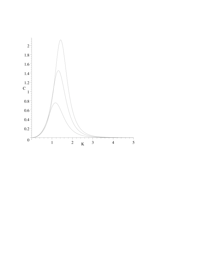
Figure 1: Specific heat (with $k_{B}\equiv 1$) for the Potts ferromagnet on the infinite-length, width $L_{y}=3$ strip of the square lattice with free transverse boundary conditions, as a function of $K=J/(k_{B}T)$. Going from bottom to top in order of the heights of the maxima, the curves are for $q=2,3,4$.

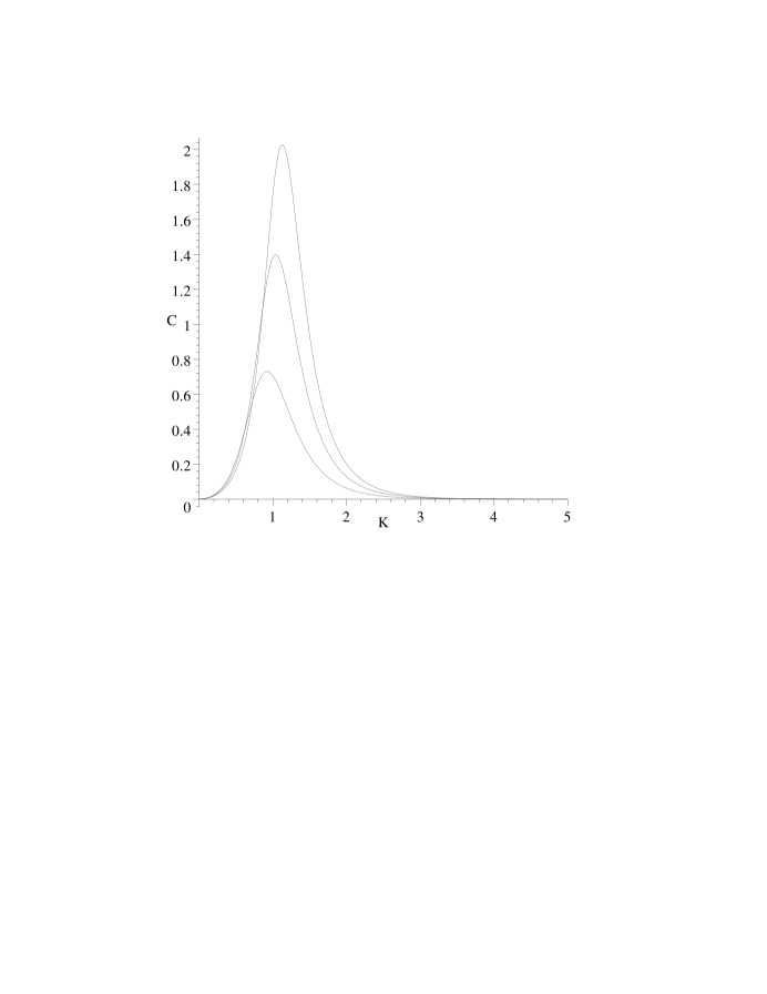
Figure 2: Specific heat (with $k_{B}\equiv 1$) for the Potts ferromagnet on the infinite-length, width $L_{y}=3$ strip of the square lattice with periodic transverse boundary conditions as a function of $K=J/(k_{B}T)$. Going from bottom to top in order of the heights of the maxima, the curves are for $q=2,3,4$.

Table 1: Some properties of the specific heat of the $q$-state Potts ferromagnet on strips of the square lattice with free and periodic transverse boundary conditions.

$q$	$BC_{y}$	$L_{y}$	$K_{C,max}$	$C_{max}/k_{B}$	$T_{C,max}/T_{c,sq}$
2	$FBC_{y}$	1	2.40	0.439	0.367
2	$FBC_{y}$	2	1.33	0.631	0.663
2	$FBC_{y}$	3	1.17	0.755	0.753
2	$PBC_{y}$	2	1.00	0.529	0.8805
2	$PBC_{y}$	3	0.92	0.729	0.958
3	$FBC_{y}$	1	2.65	0.762	0.379
3	$FBC_{y}$	2	1.49	1.167	0.676
3	$FBC_{y}$	3	1.31	1.453	0.767
3	$PBC_{y}$	2	1.12	0.943	0.899
3	$PBC_{y}$	3	1.04	1.396	0.966
4	$FBC_{y}$	1	2.84	1.023	0.386
4	$FBC_{y}$	2	1.61	1.647	0.684
4	$FBC_{y}$	3	1.42	2.119	0.774
4	$PBC_{y}$	2	1.21	1.292	0.910
4	$PBC_{y}$	3	1.13	2.026	0.972

In Figs. 1 and 2 we show plots of the specific heat for the Potts ferromagnet on the infinite-length limits of the $L_{y}=3$ strips with free and periodic transverse boundary conditions. In each curve, the specific heat assumes a maximum value $C_{max}$ at a certain value of inverse temperature $K_{C,max}$, or equivalently, temperature $T_{C,max}=J/(k_{B}K_{C,max})$. It is of interest to inquire how these quantities depend on $q$ and the transverse boundary conditions. We give this information for the results in the present paper and also our relevant previous studies [14] in Table 1. In general, for the Potts ferromagnet on the infinite-length strip of width $L_{y}$ and given transverse boundary condition, we find that, for physical $q$,

$$T_{C,max}\ \ {\rm is\ \ a\ \ decreasing\ \ function\ \ of}\ \ q$$ (4.2.1)

and

$$C_{max}\ \ {\rm is\ \ an\ \ increasing\ \ function\ \ of}\ \ q\ .$$ (4.2.2)

The monotonicity (4.2.1) can be understood as a consequence of the fact that the specific heat, $C=dU/dT$, reaches a maximum at the temperature where there is an onset of short-range order, as reflected in the maximal temperature derivative of the internal energy. As $q$ increases, there are more effective degrees of freedom per site, and hence it is necessary to cool the system to a lower temperature, i.e., higher value of $K$, to obtain short-range ordering. The monotonicity relation (4.2.2) shows that this onset of short-range order occurs more sharply as $q$ increases.

We may also study the dependence of $T_{C,max}$ and $C_{max}$ as a function of the strip width and transverse boundary conditions for the Potts ferromagnet with a given value of $q$ and investigate how $T_{C,max}$ approaches the critical value [2]

$$T_{c}=\frac{J}{k_{B}\ln(1+\sqrt{q})}\ ,$$ (4.2.3)

i.e., $a_{c}=1+\sqrt{q}$, of the model on the infinite square lattice. As summarized in Table 1, we find that, for a given (physical, integral) $q\geq 2$ and for strips considered here,

$$T_{C,max}\ \ {\rm and}\ \ C_{max}\ \ {\rm are\ \ increasing\ \ functions\ \ of}\ \ L_{y}\ .$$ (4.2.4)

For the strips with free transverse boundary conditions, the monotonicity relation (4.2.4) for $T_{C,max}$ can be explained as follows. As $L_{y}$ increases, the effective coordination number, given by (1.31) above, also increases. Since the short-range ordering is a consequence of the ferromagnetic spin-spin interactions and since, on average, a given spin feels the influence of $\Delta_{eff}$ of these interactions, a given degree of short-range order can be established at a higher temperature as $L_{y}$ increases. Since, as recalled above, the maximum in the specific heat occurs at the temperature where this onset of short range order is taking place, the monotonicity relation (4.2.4) follows. Of course, in the limit $L_{y}\to\infty$, the point $T_{C,max}$ is a true critical point at which there is a nonanalyticity in the free energy, and the specific heat does not just reach a maximum due to short-range ordering, but diverges (logarithmically) [59], with the onset of long-range order, i.e. nonzero spontaneous magnetization. For the strips with periodic transverse boundary conditions, as $L_{y}$ increases, there is no change in the coordination number $\Delta=4$; rather, there are actually two countervailing tendencies: (i) an increase in the effectiveness of short-range ordering, which, in the limit $L_{y}\to\infty$ yields long-range order at sufficiently low temperature, (ii) a decrease in the finite-size effects involving spin-spin interactions that loop around the finite transverse periodic direction. To explain (ii), consider two spins which, for simplicity, are located at the same value of $x$ but different values of $y$, $y_{1}$ and $y_{2}$. On an infinite square lattice, the leading contribution to the interaction of these spins would be via a minimum-distance path, of length $r=|y_{1}-y_{2}|$. However, for finite $L_{y}$, there is another contribution, namely via the path going the other way around the transverse direction, of length $L_{y}-r$. This is a finite-lattice artifact, the effect of which goes to zero as $L_{y}\to\infty$. For the toroidal strips considered here, the effect (i) outweighs (ii), yielding the monotonicity relation (4.2.4). This result may be compared with the results for the Ising $q=2$ case obtained by Ferdinand and Fisher [58]. These authors considered finite-size $L_{x}\times L_{y}$ lattices with toroidal boundary conditions and studied the limiting behavior of the specific heat as $L_{x}\to\infty$ and $L_{y}\to\infty$ with fixed finite nonzero ratio $L_{y}/L_{x}$. Among their other results, they showed that if this limit is taken with finite-size sections with relatively square-like aspect ratios $1/3.1\mathrel{\raisebox{-2.58334pt}{$\stackrel{{\scriptstyle\textstyle<}}{{\sim}}$}}L_{y}/L_{x}\mathrel{\raisebox{-2.58334pt}{$\stackrel{{\scriptstyle\textstyle<}}{{\sim}}$}}3.1$, then $T_{C,max}$ approaches $T_{c}$ from above in the thermodynamic limit, while for more narrow rectangular shapes, $L_{y}/L_{x}\mathrel{\raisebox{-2.58334pt}{$\stackrel{{\scriptstyle\textstyle>}}{{\sim}}$}}3.1$ or $L_{y}/L_{x}<1/3.1$, $T_{C,max}$ approaches $T_{c}$ from below. Although our finite-size studies of the $q=2$ Potts model on toroidal strips do not, strictly speaking, fall into the category considered by Ferdinand and Fisher since we take $L_{x}\to\infty$ keeping $L_{y}$ fixed, so that $L_{y}/L_{x}$ is identically zero, our results may be expected to correspond most closely to the extreme limit $L_{y}/L_{x}\to 0$ in the work of [58]. Hence, one would expect that for $q=2$ our $T_{C,max}$ should approach $T_{c}$ from below, and it does. It is of interest that our calculations generalize this monotonicity result to $q\geq 3$.

Our calculations also show that for a $q$ and given width $L_{y}$, the ratio $T_{C,max}/T_{c}$ is closer to its limit of unity if one uses a strip with periodic rather than free transverse boundary conditions. This is easily explained since periodic transverse boundary conditions remove edge effects and thereby reduce finite-size artifacts.

Although the (zero-field) free energy of the general $q$-state Potts model has not been calculated for arbitrary temperature, it has been calculated in [68] at the phase transition temperature $T_{c}$ for the ferromagnet, (4.2.3). Of course, the free energy is also known exactly for the $q=2$ Ising case. In addition to the studies of $L_{y}$-dependence and comparisons of $T_{C,max}/T_{c}$ discussed in the preceding paragraphs, it is of interest to compare our results with a conformal field theory relation concerning finite-size effects, for the $q$ values where the Potts ferromagnet has a second-order transition in 2D, namely, $q=2,3$, and 4. For this purpose, we recall that conformal field theory methods have provided insight into the universality classes of continuous, second-order phase transitions and the associated critical exponents in terms of Virasoro algebras with given central charges and scaling dimensions [62]-[64]. The Virasoro algebra with central extension depending on the central charge $c$ is

$$[L_{m},L_{n}]=(m-n)L_{m+n}+\frac{c}{12}m(m^{2}-1)\delta_{m+n,0}$$ (4.2.5)

For the values of $q$ where the 2D Potts ferromagnet has a continuous transition (with infinite correlation length), the central charges are given by [62]-[64] (i) $c=1/2$ for $q=2$, (ii) $c=4/5$ for $q=3$, and (iii) $c=1$ for $q=4$. There is a useful relation from conformal field theory that describes the approach of the free energy of an infinite strip with free or periodic transverse boundary conditions to the 2D thermodynamic limit as $L_{y}\to\infty$ at the critical temperature of the 2D model [65]-[67]:

$$f_{strip,L_{y}}=f_{bulk}+\frac{f_{surf.}}{L_{y}}+\frac{\Delta}{L_{y}^{2}}+O(L_{y}^{-3})$$ (4.2.6)

where $f_{surf.}=0$ is nonzero (zero) for free (periodic) boundary conditions in the $y$ direction and

$$\Delta=\left\{\begin{array}[]{ll}\frac{\pi}{6}c&\mbox{for PBC${}_{y}$}\\ \frac{\pi}{24}c&\mbox{for FBC${}_{y}$}\end{array}\right.$$ (4.2.7)

To compare our results with this relation, we use as input the critical values of the Potts model free energy on the square lattice. For $q=2$, from the Onsager solution [59] one has

$$f_{Potts,q=2,crit.}=\frac{1}{2}\ln 2+\ln(1+\sqrt{2}\ )+\frac{2}{\pi}G_{c}=1.811068985...$$ (4.2.8)

where $G_{C}$ is the Catalan constant

$$G_{C}=\sum_{k=0}^{\infty}\frac{(-1)^{k}}{(2k+1)^{2}}=0.91596559...$$ (4.2.9)

For $q=3$ and $q=4$, one has [68]

$$f_{Potts,q=3,crit.}=\ln 2+\frac{1}{2}\ln 3+\frac{1}{3}\ln(2+\sqrt{3}\ )+\frac{4G_{C}}{3\pi}=2.07018716...$$ (4.2.10)

and

$$f_{Potts,q=4,crit.}=-3\ln 2+4\ln\biggl{(}\frac{\Gamma(1/4)}{\Gamma(3/4)}\biggr{)}=2.25952475...$$ (4.2.11)

where $\Gamma(z)$ is the Euler Gamma function. As an illustration, we consider the width $L_{y}=3$ strip with periodic transverse boundary conditions. In Table 2 we list the values of the right-hand side of (4.2.6) and the evaluation of $f_{strip}$ at the value $T=T_{c}$ where the model is critical on the 2D lattice. Of course, for any finite value of $L_{y}$, $f_{strip}$ is not critical at this value of temperature and, for comparison, we also list the comparison with $f_{strip}$ evaluated at $T=T_{C,max}$. Clearly, as $L_{y}\to\infty$, $T_{C,max}\to T_{c}$, so that these are equivalent in this limit. One sees that eq. (4.2.6) is reasonably well satisfied, even for the modest value of the width $L_{y}=3$.

Table 2: Comparison of exact partition function calculations with conformal field theory finite-size relation for the infinite-length, width $L_{y}=3$ strip with periodic transverse boundary conditions. See text for further details.

$q$	RHS	$f_{strip}(T_{c})$	$f_{strip}(T_{C,max})$
2	1.840	1.8425	1.91
3	2.117	2.121	2.18
4	2.318	2.324	2.37

4.2.2 $T\to 0$ Limit

We next derive some general results concerning the low-temperature behavior of the (reduced) free energy $f$ and, from this, the internal energy $U$ and specific heat $C$, for the $q$-state Potts ferromagnet on an infinite-length strip of the square lattice with arbitrary longitudinal boundary conditions and specified transverse boundary conditions. For technical convenience, we use free longitudinal boundary conditions for our calculations, assume a large length $L_{x}$ when calculating the partition function, and then, as usual, take $L_{x}\to\infty$ when calculating the free energy (per site). At $T=0$, $Z=qa^{e(G)}$, where, as defined above, $e(G)$ denotes the number of edges (bonds) on the strip graph. Now consider finite-temperature corrections to this result. If the lattice were of dimensionality $d\geq 2$, the leading order term always arises from a configuration in which one changes one spin from its preferred value to one of the $(q-1)$ other values, and so forth for successive corrections. However, the leading corrections do not, in general, arise in this simple a manner for the finite-width strips, especially in the case where the transverse boundary conditions are free. Let us begin with these.

For $L_{y}=1$, the leading low-temperature correction arises from changing all of the spins to the right, say, of a given point from their previous value to one of the $(q-1)$ other values. Since this can be done at any of $L_{x}$ locations, we obtain $f=K+(q-1)e^{-K}+...$, where $...$ here and below indicate subdominant terms in the $T\to 0$ limit, and hence $U=J[-1+(q-1)e^{-K}]$ and $C=k_{B}K^{2}(q-1)e^{-K}$. Of course, in this $L_{y}=1$ case, the exact expressions for $f$, $U$, and $C$ are simple: $f=\ln(e^{K}+q-1)$, $U=-Je^{K}/(e^{K}+q-1)$, and $C=k_{B}K^{2}(q-1)e^{K}/(e^{K}+q-1)^{2}$.

For $L_{y}=2$, the leading correction to the low-temperature limit for $Z$ is obtained by changing all of the spins to the right of a given transverse slice from their original value to one among the $(q-1)$ other possibilities. This yields the expansion

$$f_{FBC_{y},L_{y}=2}=\frac{3}{2}K+\frac{1}{2}(q-1)e^{-2K}+...$$ (4.2.12)

and hence

$$U_{FBC_{y},L_{y}=2}=J\Bigl{[}-\frac{3}{2}+(q-1)e^{-2K}+...\Bigr{]}$$ (4.2.13)

and

$$C_{FBC_{y},L_{y}=2}=2k_{B}K^{2}(q-1)e^{-2K}+...$$ (4.2.14)

as given in [14], in agreement with a direct derivation from the exact results obtained therein.

For $L_{y}=3$, there are two different types of leading corrections to the low-temperature limit for $Z$, obtained by (i) changing all of the spins to the right of a given transverse slice from their original value to one among the $(q-1)$ other possibilities, and (ii) changing a spin on the upper or lower boundary from its original value to one among the $(q-1)$ others. These both involve a suppression factor $e^{-3K}$, and one gets the expansion

$$f_{FBC_{y},L_{y}=3}=\frac{5}{3}K+(q-1)e^{-3K}+...$$ (4.2.15)

and hence

$$U_{FBC_{y},L_{y}=3}=J\Bigl{[}-\frac{5}{3}+3(q-1)e^{-3K}+...\Bigr{]}$$ (4.2.16)

and

$$C_{FBC_{y},L_{y}=3}=9k_{B}K^{2}(q-1)e^{-3K}+...$$ (4.2.17)

We have that this is consistent with a direct derivation from the exact result (4.1.1).

For greater widths, $L_{y}\geq 4$, the leading low-temperature correction arises from changing one of the spins on the upper or lower horizontal edges from their original values to one of the other $(q-1)$ possible values. This makes the dominant contribution because of the fact that these edge spins have a lower coordination number (degree), namely $\Delta=3$, than the spins in the interior of the strip. We have

$$f_{FBC_{y},L_{y}\geq 4}=\frac{\Delta_{eff}}{2}K+\frac{2}{L_{y}}(q-1)e^{-3K}+...$$ (4.2.18)

where $\Delta_{eff}$ was given in eq. (1.31) above, and hence

$$U_{FBC_{y},L_{y}\geq 4}=J\Bigl{[}-\frac{\Delta_{eff}}{2}+\frac{6}{L_{y}}(q-1)e^{-3K}+...\Bigr{]}$$ (4.2.19)

and

$$C_{FBC_{y},L_{y}\geq 4}=\frac{18}{L_{y}}k_{B}K^{2}(q-1)e^{-3K}+...$$ (4.2.20)

The essential zeros in $U$ and $C$ are typical for a spin model at its lower critical dimensionality and mean that the low-temperature series expansion has zero radius of convergence. Physically, this reflects the qualitatively different behavior at $T=0$, where there is saturated magnetization, and at any nonzero temperature, regardless of how small, where this magnetization vanishes identically.

Now consider a strip of the square lattice with free transverse boundary conditions and arbitrarily great width $L_{y}\geq 3$. Let the free energy be denoted as

$$f=\frac{1}{L_{y}}\ln\lambda_{L_{y},PM}$$ (4.2.21)

where $\lambda_{L_{y},PM}$ is the term in (1.12) that is dominant for physical temperature (paramagnetic phase). Then for $L_{y}=3$ this has the low-temperature expansion

$$\lambda_{L_{y}=3,PM}=e^{5K}\Bigl{[}1+3(q-1)e^{-3K}+...\Bigr{]}$$ (4.2.22)

i.e., in the notation of eq. (1.22),

$$\lambda_{L_{y}=3,PM,u}=1+3(q-1)u^{3}+...\quad{\rm for}\ \ u\to 0$$ (4.2.23)

and for $L_{y}\geq 4$,

$$\lambda_{L_{y},PM}=e^{(\Delta_{eff}/2)L_{y}K}\Bigl{[}1+2(q-1)e^{-3K}+...\Bigr{]}$$ (4.2.24)

and hence, in the notation of eq. (1.22),

$$\lambda_{L_{y},PM,u}=1+2(q-1)u^{3}+...\quad{\rm for}\ \ u\to 0\ .$$ (4.2.25)

Since the singular locus ${\cal B}$ is defined in the neighborhood of the point $u=0$ by the degeneracy of magnitudes $|\lambda_{L_{y},PM}|=|\lambda_{L_{y},j}|$, where $\lambda_{L_{y},j}$ is another leading term at this point, it follows that this locus does not involve an arbitrarily large number of curves crossing in an intersection point at $u=0$, and the corresponding complex-temperature partition function zeros (Fisher zeros [71]) do not become dense in the vicinity of the origin as $L_{y}\to\infty$. These results supercede a conjecture given in [14].

We next derive corresponding low-temperature expansions for strips with periodic transverse boundary conditions. In the cases $L_{y}=2$ and $L_{y}=3$, the leading correction term arises from changing all of the spins to the right of a transverse slice from their original values to one of $(q-1)$ other values. This yields

$$f_{PBC_{y},L_{y}}=2K+\frac{1}{L_{y}}(q-1)e^{-L_{y}K}+...$$ (4.2.26)

$$U_{PBC_{y},L_{y}}=J\Bigl{[}-2+(q-1)e^{-L_{y}K}+...\Bigr{]}$$ (4.2.27)

$$C_{PBC_{y},L_{y}}=L_{y}k_{B}K^{2}(q-1)e^{-L_{y}K}+...$$ (4.2.28)

For $L_{y}=4$, these spin configurations involving a seam make a contribution equal to those from configurations in which one changes one of the spins on a transverse slice to one of $(q-1)$ other values, so that

$$f_{PBC_{y},L_{y}=4}=2K+\frac{5}{4}(q-1)e^{-4K}+...$$ (4.2.29)

$$U_{PBC_{y},L_{y}=4}=J\Bigl{[}-2+5(q-1)e^{-4K}+...\Bigr{]}$$ (4.2.30)

$$C_{PBC_{y},L_{y}=4}=20k_{B}K^{2}(q-1)e^{-4K}+...$$ (4.2.31)

Finally, for $L_{y}\geq 5$, the leading correction term in the low-temperature limit arises in the same way as on an infinite 2D square lattice with toroidal boundary conditions, namely via the change of a single spin to one of $(q-1)$ other values. This yields expansions whose leading term is the same as on the infinite square lattice:

$$f_{PBC_{y},L_{y}\geq 5}=2K+(q-1)e^{-4K}+...$$ (4.2.32)

$$U_{PBC_{y},L_{y}\geq 5}=J\Bigl{[}-2+4(q-1)e^{-4K}+...\Bigr{]}$$ (4.2.33)

$$C_{PBC_{y},L_{y}\geq 5}=16k_{B}K^{2}(q-1)e^{-4K}+...$$ (4.2.34)

Next consider a strip of the square lattice with periodic transverse boundary conditions and arbitrarily great width $L_{y}\geq 5$. Let the free energy be denoted as in (4.2.21). Then we have the low-temperature expansion

$$\lambda_{L_{y},PM}=e^{2L_{y}K}\Bigl{[}1+L_{y}(q-1)e^{-4K}+...\Bigr{]}$$ (4.2.35)

i.e., in the notation of eq. (1.22),

$$\lambda_{L_{y},PM,u}=1+L_{y}(q-1)u^{4}+...\quad{\rm for}\ \ u\to 0\ .$$ (4.2.36)

4.3 Potts Antiferromagnet

4.3.1 Free Energy, Specific Heat, and Approach to Square Lattice Limit

In the case of the Potts antiferromagnet, as discussed in [14, 15], there can be nonanalyticities at sufficiently small non-integral $q$ and temperature, but these do not represent physical phase transitions and involve a number of pathologies such as non-existence of a thermodynamic limit independent of longitudinal boundary conditions, negative specific heats, and lack of a Gibbs measure. For the physical cases, the analyticity of the free energy is a consequence of the general theorem that one-dimensional and quasi-one-dimensional spin systems with short-range spin-spin interactions do not have a finite-temperature phase transition, which, in turn, is proved by an elementary application of a Peierls argument. This analyticity property is equivalent to the property that the singular locus ${\cal B}_{u}$ does not cross the positive real $u$ axis.

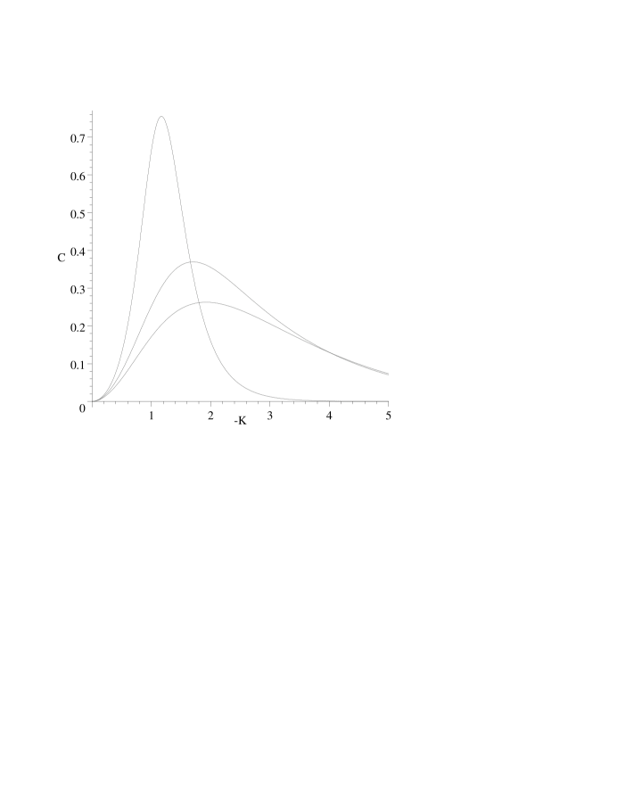
Figure 3: Specific heat (with $k_{B}\equiv 1$) for the Potts antiferromagnet on the infinite-length, width $L_{y}=3$ strip of the square lattice with free transverse boundary conditions, as a function of $K=J/(k_{B}T)$. Going from top to bottom in order of the heights of the maxima, the curves are for $q=2,3,4$.

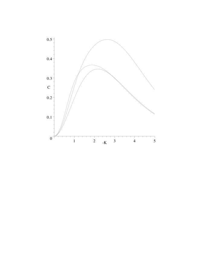
Figure 4: Specific heat (with $k_{B}\equiv 1$) for the Potts antiferromagnet on the infinite-length, width $L_{y}=3$ strip of the square lattice, as a function of $K=J/(k_{B}T)$. Going from top to bottom in order of the heights of the maxima, the curves are for $q=3,2,4$.

Table 3: Some properties of the specific heat of the $q$-state Potts antiferromagnet on strips of the square lattice with free and periodic transverse boundary conditions. Since for $q\geq 3$ this model has no finite-temperature phase transition on the square lattice, the last column is left blank.

$q$	$BC_{y}$	$L_{y}$	$-K_{C,max}$	$C_{max}/k_{B}$	$T_{C,max}/T_{c,sq}$
2	$FBC_{y}$	1	2.40	0.439	0.367
2	$FBC_{y}$	2	1.33	0.631	0.663
2	$FBC_{y}$	3	1.17	0.755	0.753
2	$PBC_{y}$	2	1.00	0.529	0.8805
2	$PBC_{y}$	3	1.88	0.366	0.469
3	$FBC_{y}$	1	2.23	0.241	$-$
3	$FBC_{y}$	2	1.785	0.3325	$-$
3	$FBC_{y}$	3	1.70	0.369	$-$
3	$PBC_{y}$	2	1.33	0.287	$-$
3	$PBC_{y}$	3	2.62	0.498	$-$
4	$FBC_{y}$	1	2.16	0.166	$-$
4	$FBC_{y}$	2	1.96	0.238	$-$
4	$FBC_{y}$	3	1.92	0.263	$-$
4	$PBC_{y}$	2	1.49	0.208	$-$
4	$PBC_{y}$	3	2.16	0.346	$-$

In Figs. 3 and 4 we show plots of the specific heat for the Potts antiferromagnet on the infinite-length limits of the $L_{y}=3$ strips with free and periodic transverse boundary conditions. Using our exact results, we have calculated similar plots for $L_{y}=2$, but to save space we do not show them here. In Table 3 we list some comparative information on $K_{C,max}$ and $C_{max}$ from our previous and current exact calculations. In contrast to the situation with the ferromagnet, $|K_{C,max}|$ does not have a uniform behavior with respect to $q$; for example, for the strips with free transverse boundary conditions, for $L_{y}=1$, it decreases with increasing $q$ while for $L_{y}=2$ and $L_{y}=3$ it increases with increasing $q$. For the strips with periodic transverse boundary conditions, $|K_{C,max}|$ increases with increasing $q$ for $L_{y}=2$ but is not a monotonic function of $q$ for $L_{y}=3$. Note that for the $q=2$ Ising value on the $L_{y}=3$ strip with periodic boundary conditions the frustration affects the value of $K_{C,max}$; this would also be true on wider strips of this type with odd $L_{y}$. For fixed $q$, as a function of $L_{y}$, we find that for the strips with free transverse boundary conditions, $|K_{C,max}|$ decreases and $C_{max}$ increases as $L_{y}$ increases; for the strips with periodic boundary conditions these trends also apply for $q\geq 3$, but for $q=2$, one encounters the effects of frustration for $L_{y}=3$ and, more generally, for odd $L_{y}$. Since the $q=3$ Potts antiferromagnet has a zero-temperature critical point on the square lattice, one can make use of the relation (4.2.6) from conformal field theory. In this case the model exhibits ground state entropy without frustration, and, since $\lim_{T\to 0}\beta U=0$, the general relation $f=-\beta U+S/k_{B}$ (i.e., $F=U-TS$) reduces to $f=S_{0}/k_{B}$. Hence, eq. (4.2.6) becomes

$$S_{strip,L_{y}}=S_{bulk}+\frac{S_{surf.}}{L_{y}}+\frac{\Delta}{L_{y}^{2}}+O(L_{y}^{-3})\ .$$ (4.3.1)

Using the exact calculation of the ground state entropy for the $L_{y}=4$ strip with cylindrical boundary conditions [35], it was noted earlier [42] that this relation is satisfied quite well for the known value of the central charge, $c=1$.

4.3.2 $T\to 0$ Limit

As regards the low-temperature expansions of the internal energy and specific heat for the antiferromagnetic Potts model on these strips, these depend on $q$ in a more complicated manner than the analogous expansions for the ferromagnetic case, as was already clear from eqs. (6.35)-(6.37) and (6.39) in [14]. For the Ising value $q=2$ on strips of the square lattice with free transverse boundary conditions, the limit $L_{x}\to\infty$ can always be taken such that the graphs are bipartite, and hence the correction terms in $U$ and $C$ are obtained from those for the ferromagnet by the replacement $K\to-K$. However, for other values of $q$, the dependence is, in general, different. For example, for $L_{y}=2$, $C$ has an exponential factor $e^{2K}$ if $q=2$ but $e^{K}$ if $q\neq 2$ [14].

5 Locus ${\cal B}$ for the $L_{y}=3$ Strip with Cyclic or Möbius Boundary Conditions

5.1 ${\cal B}$ in the $q$ Plane

The singular locus ${\cal B}$ in the $q$ plane was given in [46] for the special case $a=0$, i.e., the zero-temperature Potts antiferromagnet. This locus separates the $q$ plane into seven regions. The first of these is $R_{1}$, which includes the real intervals $q<0$ and $q>q_{c}$, where

$$q_{c}=2.33654..\quad{\rm for}\ \ a=0,\ \ G=sq,\ L_{y}=3,\ FBC_{y},\ (T)PBC_{x}\ .$$ (5.1.1)

The other regions are $R_{2}$, including the real interval $2<q<q_{c}$; $R_{3}$ including the real interval $0<q<2$; two complex-conjugate (c.c.) phases $R_{4},R_{4}^{*}$ centered at $q\simeq 2.4\pm 0.9i$; and two additional quite narrow, sliver-like c.c. phases $R_{5},R_{5}^{*}$ centered at $q\simeq 1.93\pm 1.70i$. In region $R_{1}$ the dominant $\lambda$ is, with our current ordering of terms, $\lambda_{P,s3c,9}$, so that for either cyclic or Möbius longitudinal boundary conditions,

$$W(sq,3\times\infty,FBC_{y},(T)PBC_{x},q)=(\lambda_{P,s3c,9})^{1/3}\quad{\rm for}\ \ q\in R_{1}\ .$$ (5.1.2)

In region $R_{2}$, the dominant $\lambda$ is $q-4$, so

$$|W(sq,3\times\infty,FBC_{y},(T)PBC_{x},q)|=|q-4|^{1/3}\quad{\rm for}\quad q\in R_{2}\ .$$ (5.1.3)

Recall that for regions other than $R_{1}$, only the magnitude of $W$ can be determined unambiguously [24]. In region $R_{3}$, the dominant $\lambda$ is the maximal root of the cubic (2.3.8). In the complex conjugate pairs of regions ($R_{4},R_{4}^{*}$) and ($R_{5},R_{5}^{*}$) the dominant $\lambda$’s are the other two roots of the cubic (2.3.8). In each of these regions, $|W|=|\lambda_{P,s3c,j,dom.}|^{1/3}$, where $\lambda_{P,s3c,j,dom.}$ is the dominant root in the respective region.

Figure 5: Singular locus ${\cal B}$ in the $q$ plane for the free energy of the Potts antiferromagnet for the temperature given by $a=0.1$, i.e., $K=-\ln 10$, on the width $L_{y}=3$, infinite-length strip of the square lattice with cyclic or Möbius boundary conditions. Partition function zeros for the cyclic strip with length $L_{x}=20$ and thus $n=60$ vertices are shown for comparison.

Figure 6: Singular locus ${\cal B}$ in the $q$ plane for the free energy of the Potts antiferromagnet for the temperature given by $a=0.5$, i.e., $K=-\ln 2$, on the width $L_{y}=3$, infinite-length strip of the square lattice with cyclic or Möbius boundary conditions. Partition function zeros for the cyclic strip with length $L_{x}=20$ and thus $n=60$ vertices are shown for comparison.

In Figs. 5 and 6 we show plots of the locus ${\cal B}_{q}$ for the Potts antiferromagnet at the values of temperature given by $a=0.1$, i.e., $K=-\ln 10$, and $a=0.5$, i.e., $K=-\ln 2$. For comparison, typical sets of partition function zeros in the $q$ plane are shown for long finite strips. As $a$ increases from 0 to 1, i.e., the temperature increases from 0 to infinity for the Potts antiferromagnet, the boundary ${\cal B}_{q}$ contracts and finally shrinks to a point at the origin in the $q$ plane. In the interval $0\leq a\leq a_{crc}$, where $a_{crc}=0.181720..$, the rightmost part of the boundary and hence also $q_{c}$ sweep to the left, while the crossing at $q=2$ remains; at $a=a_{crc}$, the rightmost part of the boundary coincides with $q=2$, i.e., $q_{c}=2$. As $a$ increases further in the interval $a_{crc}\leq a\leq 1$, there are only two regions, $R_{1}$ and $R_{3}$ that include real intervals. For this full range of temperatures in the Potts antiferromagnet, $0\leq a\leq 1$, the boundary ${\cal B}$ always passes through $q=0$.

Figure 7: Singular locus ${\cal B}$ in the $q$ plane for the free energy of the Potts ferromagnet for the temperature given by $a=2$, i.e., $K=\ln 2$, on the width $L_{y}=3$, infinite-length strip of the square lattice with cyclic or Möbius boundary conditions. Partition function zeros for the cyclic strip with length $L_{x}=20$ and thus $n=60$ vertices are shown for comparison.

In Fig. 7 we show the locus ${\cal B}_{q}$ for a typical ferromagnetic value, $a=2$, i.e. $K=\ln 2$. One can discern very small prongs extending in northwest and southwest directions from the main curve at $q\simeq-2.74\pm 1.88i$, and a short line segment on the negative real $q$ axis. Two general features are that the locus ${\cal B}$ (i) passes through $q=0$ and (ii) does not cross the positive real.

5.2 ${\cal B}$ in the $u$ Plane

Figure 8: Singular locus ${\cal B}$ in the $u$ plane for the free energy of the Potts model for $q=2$, on the width $L_{y}=3$, infinite-length strip of the square lattice with cyclic or Möbius boundary conditions. Partition function zeros for the cyclic strip with length $L_{x}=20$ and hence $e=100$ are shown for comparison.

Figure 9: Singular locus ${\cal B}$ in the $u$ plane for the free energy of the Potts model for $q=3$, on the width $L_{y}=3$, infinite-length strip of the square lattice with cyclic or Möbius boundary conditions. Partition function zeros for the cyclic strip with length $L_{x}=20$ and hence $e=100$ are shown for comparison.

Figure 10: Singular locus ${\cal B}$ in the $a=u^{-1}$ plane for the free energy of the Potts model for $q=3$, on the width $L_{y}=3$, infinite-length strip of the square lattice with cyclic or Möbius boundary conditions. Partition function zeros for the cyclic strip with length $L_{x}=20$ and hence $e=100$ are shown for comparison.

Figure 11: Singular locus ${\cal B}$ in the $u$ plane for the free energy of the Potts model for $q=10$, on the width $L_{y}=3$, infinite-length strip of the square lattice with cyclic or Möbius boundary conditions. Partition function zeros for the cyclic strip with length $L_{x}=20$ and hence $e=100$ are shown for comparison.

In Figs. 8-11 we show plots of the singular locus ${\cal B}$ for the Potts model free energy for $q=2,3$, and 10, respectively, in the infinite-length limit of the $L_{y}=3$ strip graph with cyclic or Möbius boundary conditions. Zeros of the partition function are shown for comparison. There are several interesting features of these plots. In each, there are six curves forming three branches on ${\cal B}$ that intersect at the origin, $u=0$, at the angles $\pm\pi/6$, $\pm\pi/2$, and $\pm 5\pi/6$. In general, the density of complex-temperature Fisher zeros along the curves comprising ${\cal B}$ in the vicinity of a generic singular point $u_{s}$ behaves as [71, 72]

$$g\sim|u-u_{s}|^{1-\alpha_{s}}$$ (5.2.1)

where $\alpha_{s}$ ($\alpha_{s}^{\prime}$) denotes the corresponding specific heat exponent for the approach to $u_{s}$ from within the CTE PM (FM) phase. Thus, for a continuous, second-order transition, with $\alpha_{s}<1$, this density vanishes as one approaches the critical point $u_{s}$ along ${\cal B}$. The specific heat for these infinite-length, finite-width strips has an essential zero at $T=0$ which, if expressed in terms of an algebraic specific exponent $\alpha$, corresponds to $\alpha=-\infty$ at $u=u_{s}=0$. Substituting this into (5.2.1), it follows that the density vanishes rapidly as one approaches the origin $u=0$ along the curves forming ${\cal B}_{u}$. This is evident in Figs. 8-11. As we have discussed in our earlier works on ${\cal B}$ in the $q$ and $u$ plane, any mapping of the regions in these respective planes is done with finite resolution and does not exclude the possibility of extremely small regions. That such regions can occur was evident, e.g., in [46].

In earlier work [74, 14, 15, 16, 17], it was shown that although the physical thermodynamic properties of a discrete spin model are, in general, different in quasi-1D systems such as infinite-width, finite-width strips, and in higher dimensions, nevertheless, exact solutions for ${\cal B}_{u}$ in quasi-1D systems can give insight into ${\cal B}_{u}$ in 2D. This was shown, in particular, for the $q=2$ Ising special case of the Potts model, where the comparison can be made rigorously since the model is exactly solvable in 2D. Our current results extend this comparison to greater width. For example, in the complex-temperature phase diagram of the Ising model on the square lattice, the singular locus ${\cal B}$ forms two circles $u=\pm 1+\sqrt{2}e^{i\phi}$, $0\leq\phi<2\pi$ [71, 70]. This locus thus exhibits complex-conjugate multiple points at $u=\pm i$, where four curves forming two branches on ${\cal B}$ intersect. This was also true of the Ising model on the infinite-length, width $L_{y}=2$ cyclic or Möbius strips of the square lattice [13, 14].

For the $q=2$ (Ising) case shown in Fig. 8, the locus ${\cal B}$ is invariant under the inversion mapping $u\to 1/u=a$. This is a consequence of the fact that the infinite-length limit can be taken on a sequence of bipartite graphs. It follows that the six curves extending outward to infinity in the $u$ plane cross at the origin of the $a$ plane. Thus, the points $u=0$ and $a=0$ are multiple points on ${\cal B}$. There are also complex-conjugate multiple points at $u=\pm i$, where again six curves forming three branches of ${\cal B}$ cross each other. Finally, there is another multiple point at $u=-1$ where four curves forming two branches intersect. Although the locus ${\cal B}$ does not appear to contain any arc endpoints for $q=2$, such endpoints are present for the other illustrative values of $q$, namely $q=3$ and $q=10$.

In the $q=3$ case, the intersection points of the various curves include the complex-conjugate pair $u=e^{\pm 2\pi i/3}$ as well as a negative real point, $u=-1/2$. The intersection points include both those where several curves cross and those where curves come together in a $T$-type intersection point. A previous analytic discussion of such $T$-type intersection points in complex-temperature phase diagrams was given in [73]. Besides the origin, $u=0$, the locus ${\cal B}$ crosses the real $u$ axis also at the three points $u=-2$, $u\simeq-1.37$, and $u\simeq-1.21$. We recall that for $q=3$ Potts model on the infinite-length, width $L_{y}=2$ cyclic or Möbius strip of the square lattice, ${\cal B}$ also included multiple points at $u=e^{\pm 2\pi i/3}$ and crossed the real axis at $u=-2$ and $u=-1/2$ (as well as the origin) [14]. These results for the $L_{y}=2$ and $L_{y}=3$ cyclic/Möbius strips suggest that it is likely that for the infinite 2D square lattice, ${\cal B}$ passes through the points $u=e^{\pm 2\pi i/3}$. Calculations of Fisher zeros on finite lattices show considerable scatter in the region $Re(a)<0$ [76, 77, 79] but are consistent with this suggestion. The crossings at $u=-1/2$, i.e., $a=-2$, for ${\cal B}$ on these $L_{y}=2,3$ strips are of interest since, given that the $q=3$ Potts antiferromagnet has a zero-temperature critical point on the square lattice, so that the singular locus ${\cal B}$ passes through $a=0$, it follows by duality that this locus also passes through $a=-2$ [79]. Since some features of ${\cal B}$ are clearer when it is shown in the $a=u^{-1}$ plane, we do this in Fig. 10.

The plot of ${\cal B}$ for $q=10$ plot in Fig. 11 shows another interesting feature: a portion of this locus, and the associated partition function zeros exhibit an approximately circular shape. Of course the actual locus is considerably more complicated than a circle. However, in this context, one may recall that in the $q\to\infty$ limit, the complex-temperature phase boundary is $|\zeta|=1$, where $\zeta=(a-1)/\sqrt{q}$ [78], which, for large $q$, yields the locus $|u|\to 1/\sqrt{q}$ in the $u$ plane. Thus, aside from the features of ${\cal B}$ that reflect the quasi-1D nature of the strip, such as the curves passing through $u=0$, the width $L_{y}=3$ is large enough so that one can begin to see this feature of the $q\to\infty$ limit.

6 Locus ${\cal B}$ for $L_{y}=2$ Strip with Torus/Klein Bottle Boundary Conditions

We find that the locus ${\cal B}_{q}$ for the (infinite-length limit of the) $L_{y}=2$ strip with torus or Klein bottle boundary conditions is generally similar to that for the same strip with cyclic or Möbius boundary conditions [14]. For the finite-temperature ferromagnet this is again true. In particular, ${\cal B}_{q}$ for the ferromagnet does not cross the positive real $q$ axis.

In Figs. 12 and 13 we plot ${\cal B}_{u}$ for $q=2$ and $q=3$. These loci contain four curves forming two branches that cross at the origin, with angles $\pm\pi/4$ and $\pm 3\pi/4$. Comparing the locus for $q=2$ plot with the corresponding locus in the case of the infinite-length $L_{y}=2$ cyclic or Möbius strip of the square lattice [14, 15] we observe that here the locus is symmetric under the map $u\to-u$, whereas for the cyclic or Möbius strip it is not. The reason for this is that the torus or Klein bottle strip has an even coordination number, $\Delta=4$, whereas the cyclic or Möbius strip has an odd coordination number, $\Delta=3$ (both are $\Delta$-regular graphs). The $q=3$ locus contains intersection points at $u=e^{\pm 2\pi i/3}$ as well as two pairs of $T$ (equivalently, $Y$) type intersection points, and crosses the negative real axis at $u=-1$ and $u=-2$.

Figure 12: Singular locus ${\cal B}$ in the $u$ plane for the free energy of the Potts model for $q=2$, on the width $L_{y}=2$, infinite-length strip of the square lattice with torus or Klein bottle boundary conditions. Partition function zeros for the toroidal strip with length $L_{x}=20$ and hence $e=80$ are shown for comparison.

Figure 13: Singular locus ${\cal B}$ in the $u$ plane for the free energy of the Potts model for $q=3$, on the width $L_{y}=2$, infinite-length strip of the square lattice with torus or Klein bottle boundary conditions. Partition function zeros for the toroidal strip with length $L_{x}=20$ ($e=80$) are shown for comparison.

7 Locus ${\cal B}$ for $L_{y}=3$ Strip with Torus/Klein Bottle Boundary Conditions

7.1 ${\cal B}$ in the $q$ Plane

Figure 14: Singular locus ${\cal B}$ in the $q$ plane for the free energy of the zero-temperature Potts antiferromagnet on the $L_{y}=3$ strip of the square lattice with torus or Klein bottle boundary conditions. Chromatic zeros for the toroidal strip with length $L_{x}=30$ and thus $n=90$ vertices are shown for comparison.

Figure 15: Singular locus ${\cal B}$ in the $q$ plane for the free energy of the Potts antiferromagnet for the temperature given by $a=0.1$, i.e., $K=-\ln 10$, on the width $L_{y}=3$, infinite-length strip of the square lattice with torus or Klein bottle boundary conditions. Partition function zeros for the toroidal strip with length $L_{x}=20$ and thus $n=60$ vertices are shown for comparison.

Figure 16: Singular locus ${\cal B}$ in the $q$ plane for the free energy of the Potts antiferromagnet for the temperature given by $a=0.5$, i.e., $K=-\ln 2$, on the width $L_{y}=3$, infinite-length strip of the square lattice with torus or Klein bottle boundary conditions. Partition function zeros for the toroidal strip with length $L_{x}=20$ and thus $n=60$ vertices are shown for comparison.

For comparison with our finite-temperature results, we show in Fig. 14 the locus ${\cal B}$ for the infinite-length limit of the $L_{y}=3$ strip with torus or Klein bottle boundary conditions in the $q$ plane for $a=0$, i.e., the zero-temperature Potts antiferromagnet, on the $L_{y}=3$ strip of the square lattice with torus or Klein bottle boundary conditions [51]. This locus separates the $q$ plane into three regions: $R_{1}$ including the real intervals $q>q_{c}$, where $q_{c}=3$, and $q<0$ and extending to arbitrarily large $|q|$; $R_{2}$, including the real interval $2<q<3$, and (iii) $R_{3}$, including the real interval $0<q<2$. Thus, ${\cal B}_{q}$ crosses the real $q$ axis at $q=0,2$, and 3. For the same model at the finite values of temperature given by $a=0.1$ and $a=0.5$, we show ${\cal B}_{q}$ in Figs. 15 and 16. As $a$ increases from 0 to 1, i.e., the temperature increases from 0 to infinity for the Potts antiferromagnet, the boundary ${\cal B}_{q}$ contracts to a point at the origin in the $q$ plane. In the interval $0\leq a\leq a_{cr}$, where $a_{cr}=0.3488338...$, which is a root of the equation

$$2z^{12}+13z^{11}+21z^{10}+38z^{9}+46z^{8}-11z^{7}+40z^{6}$$ (7.1.1)

(7.1.2)

$$-17z^{5}+44z^{4}-70z^{3}+35z^{2}-17z+4=0\ .$$ (7.1.3)

The boundary between regions $R_{2}$ and $R_{3}$ remains fixed at $q=2$ and the right-most part of the boundary, passing through $q_{c}$ and separating $R_{1}$ and $R_{2}$ moves leftward, and crosses $q=2$ at $a=a_{cr}$. In the interval $a_{cr}<a<1$, there are only two regions, $R_{1}$ and $R_{3}$, that contain intervals of the real axis, and $q_{c}$ continues to decrease from 2 to 0.

In Fig. 17 we show the locus ${\cal B}_{q}$ for a typical ferromagnetic value, $a=v+1=2$, i.e. $K=\ln 2$. As is evident in this figure, ${\cal B}$ includes a complex-conjugate pair of prongs extending outward from the main curve.

Figure 17: Singular locus ${\cal B}$ in the $q$ plane for the free energy of the Potts ferromagnet for the temperature given by $a=2$, i.e., $K=\ln 2$, on the width $L_{y}=3$, infinite-length strip of the square lattice with torus or Klein bottle boundary conditions. Partition function zeros for the toroidal strip with length $L_{x}=20$ and thus $n=60$ vertices are shown for comparison.

7.2 ${\cal B}$ in the $u$ Plane

We show here plots of the singular locus ${\cal B}$ and partition function zeros in the $u=1/a$ plane for several illustrative values of $q$, namely, $q=2$, $q=3$, and $q=10$ in Figs. 18- 20.

Figure 18: Singular locus ${\cal B}$ in the $u$ plane for the free energy of the Potts model for $q=2$, on the width $L_{y}=3$, infinite-length strip of the square lattice with torus or Klein bottle boundary conditions. Partition function zeros for the toroidal strip with length $L_{x}=15$ and hence $e=90$ are shown for comparison.

Figure 19: Singular locus ${\cal B}$ in the $u$ plane for the free energy of the Potts model for $q=3$, on the width $L_{y}=3$, infinite-length strip of the square lattice with torus or Klein bottle boundary conditions. Partition function zeros for the toroidal strip with length $L_{x}=20$ and hence $e=120$ are shown for comparison.

Figure 20: Singular locus ${\cal B}$ in the $u$ plane for the free energy of the Potts model for $q=10$, on the width $L_{y}=3$, infinite-length strip of the square lattice with torus or Klein bottle boundary conditions. Partition function zeros for the toroidal strip with length $L_{x}=20$ and hence $e=120$ are shown for comparison.

Some of the features of these plots are similar to those discussed above for the infinite-length $L_{y}=3$ strips of the cyclic or Möbius strips, such as the sixfold crossing of curves at $u=0$ with density of Fisher zeros rapidly vanishing near this point, and the additional multiple points at $u=\pm i$ for $q=2$ and at $u=e^{\pm 2\pi i/3}$ for $q=3$. Note that in the present case, for $q=3$, ${\cal B}$ crosses the real $u$ axis at the points $u=-1$ and $u=-(1+\sqrt{3}/)2\simeq-1.366...$, in addition to the origin. In contrast to the $L_{y}=3$ cyclic or Möbius strips, where ${\cal B}$ is compact in the $u$ plane, here, for the torus or Klein bottle strips, two complex-conjugate curves on ${\cal B}$ extend to complex infinity in the $u$ plane, i.e., pass through the origin of the $a$ plane. This is equivalent to the property shown in [51] that ${\cal B}$ for the zero-temperature (i.e., $a=0$) Potts antiferromagnet passes through $q=q_{c}=3$. As was noted in [51], this is interesting, since it indicates that the $q=3$ Potts antiferromagnet has a zero-temperature critical point on the infinite-length, width $L_{y}=3$ strips of the square lattice with torus or Klein bottle boundary conditions. As we have discussed before, a convenient feature of strips with periodic longitudinal boundary conditions is that for the $q$-state Potts antiferromagnet with a value of $q=q_{c}$ where the model has a zero-temperature critical point, this is signalled explicitly by the properties that ${\cal B}_{a}$ passes through the origin of the $a$ plane and ${\cal B}_{q}$ passes through $q=q_{c}$ for $a=0$. In contrast, if one uses strips with free longitudinal boundary conditions, this connection is not evident in general. Thus, if one uses a cylindrical rather than toroidal or Klein bottle strip with $L_{y}=3$, then the boundary ${\cal B}_{q}$ does not pass through $q=3$ [35].

8 Conclusions

In this paper we have presented and discussed exact calculations of the partition function of the $q$-state Potts model for general $q$ and temperature on strips of the square lattice of width $L_{y}=3$ vertices and arbitrary length $L_{x}$ with longitudinal boundary conditions of the cyclic, Möbius, torus, and Klein bottle types. In the infinite-length limit we analyzed the resultant thermodynamic properties and also derived a number of low-temperature expansions, including results valid for arbitrarily wide strips with free or periodic transverse boundary conditions. A number of interesting results were given for the continuous locus ${\cal B}$ where the free energy is singular in both the $q$ plane and temperature variable plane. We also discussed the related Tutte polynomials.

Acknowledgment: This research was supported in part by the U. S. NSF grant PHY-97-22101.

9 Appendix

9.1 Equations for $\lambda_{Z,s3,j}$

The terms $\lambda_{Z,s3c,j}$ for $10\leq j\leq 15$ in eq. (2.2.1) and (2.2.2) are roots of the sixth degree equation

$$\xi^{6}+f_{61}\xi^{5}+f_{62}\xi^{4}+f_{63}\xi^{3}+f_{64}\xi^{2}+f_{65}\xi+f_{66}=0$$ (9.1.1)

where

$$f_{61}=-v(7v^{3}+18v^{2}+v^{2}q+10qv+2q^{2}+v^{4})$$ (9.1.2)

$$f_{62}=v^{2}(q^{4}+12q^{3}v+2q^{3}v^{2}+v^{6}q+14v^{5}q+2v^{4}q^{2}+2v^{7}+19v^{6}$$ (9.1.3)

(9.1.4)

$$+78v^{4}+64v^{5}+109qv^{3}+54q^{2}v^{2}+66v^{4}q+20v^{3}q^{2})$$ (9.1.5)

$$f_{63}=-v^{4}(v+q)(2q^{4}+21q^{3}v+13q^{3}v^{2}+8v^{6}q+62v^{5}q+19v^{4}q^{2}+16v^{7}$$ (9.1.6)

(9.1.7)

$$+79v^{6}+126v^{4}+v^{8}+q^{4}v+q^{3}v^{3}+2v^{5}q^{2}+168v^{5}+168qv^{3}+91q^{2}v^{2}$$ (9.1.8)

(9.1.9)

$$+182v^{4}q+79v^{3}q^{2})$$ (9.1.10)

$$f_{64}=v^{6}(v+1)(v+q)^{2}(q^{4}+13q^{3}v+5q^{3}v^{2}+2v^{6}q+26v^{5}q+7v^{4}q^{2}+3v^{7}$$ (9.1.11)

(9.1.12)

$$+27v^{6}+78v^{4}+q^{3}v^{3}+77v^{5}+110qv^{3}+56q^{2}v^{2}+89v^{4}q+33v^{3}q^{2})$$ (9.1.13)

$$f_{65}=-v^{9}(v+q)^{4}(v+1)^{2}(18v^{2}+11qv+7v^{2}q+3v^{4}+qv^{3}+14v^{3}+q^{2}v+2q^{2})$$ (9.1.14)

$$f_{66}=v^{12}(v+q)^{6}(v+1)^{4}\ .$$ (9.1.15)

The terms $\lambda_{Z,s3c,j}$ for $17\leq j\leq 20$ are roots of the quartic equation

$$\xi^{4}+f_{41}\xi^{3}+f_{42}\xi^{2}+f_{43}\xi+f_{44}=0$$ (9.1.16)

where

$$f_{41}=-(15v^{3}+6v^{4}+qv^{3}+12v^{2}q+5q^{2}v+q^{3}+v^{5})$$ (9.1.17)

$$f_{42}=v^{2}(v+q)(2q^{3}+32v^{3}+30v^{2}q+v^{6}+30v^{4}+8q^{2}v^{2}+13q^{2}v+4v^{4}q$$ (9.1.18)

(9.1.19)

$$+v^{3}q^{2}+q^{3}v+21qv^{3}+10v^{5})$$ (9.1.20)

$$f_{43}=-v^{4}(v+1)(v+q)^{2}(q^{3}+15v^{3}+19v^{2}q+10v^{4}+4q^{2}v^{2}+9q^{2}v$$ (9.1.21)

(9.1.22)

$$+2v^{4}q+v^{3}q^{2}+10qv^{3}+2v^{5})$$ (9.1.23)

$$f_{44}=v^{7}(v+q)^{5}(v+1)^{3}\ .$$ (9.1.24)

9.2 Relations Between Potts Partition Function and Tutte Polynomial

The formulas relating the Potts model partition function $Z(G,q,v)$ and the Tutte polynomial $T(G,x,y)$ were given in [14] and hence we shall be brief here. The Tutte polynomial of $G$, $T(G,x,y)$, is given by [7]-[9]

$$T(G,x,y)=\sum_{G^{\prime}\subseteq G}(x-1)^{k(G^{\prime})-k(G)}(y-1)^{c(G^{\prime})}$$ (9.2.1)

where $k(G^{\prime})$, $e(G^{\prime})$, and $n(G^{\prime})=n(G)$ denote the number of components, edges, and vertices of $G^{\prime}$, and

$$c(G^{\prime})=e(G^{\prime})+k(G^{\prime})-n(G^{\prime})$$ (9.2.2)

is the number of independent circuits in $G^{\prime}$. For the graphs of interest here, $k(G)=1$. Now let

$$x=1+\frac{q}{v}$$ (9.2.3)

and

$$y=a=v+1$$ (9.2.4)

so that

$$q=(x-1)(y-1)\ .$$ (9.2.5)

Then

$$Z(G,q,v)=(x-1)^{k(G)}(y-1)^{n(G)}T(G,x,y)\ .$$ (9.2.6)

For a planar graph $G$ the Tutte polynomial satisfies the duality relation

$$T(G,x,y)=T(G^{*},y,x)$$ (9.2.7)

where $G^{*}$ is the (planar) dual to $G$. As discussed in [14], the Tutte polynomial for recursively defined graphs comprised of $m$ repetitions of some subgraph has the form

$$T(G_{m},x,y)=\sum_{j=1}^{N_{T,G,\lambda}}c_{T,G,j}(\lambda_{T,G,j})^{m}\ .$$ (9.2.8)

9.3 Cyclic and Möbius $L_{y}=3$ Strips of the Square Lattice

We calculate

$$T(sq,3\times m,FBC_{y},PBC_{x},x,y)=\sum_{j=1}^{20}c_{T,s3c,j}(\lambda_{T,s3c,j})^{m}$$ (9.3.1)

(do not confuse the $x$ and $y$ referring to the longitudinal and transverse directions with the $x$ and $y$ variables defined in (9.2.3) and (9.2.4)) and

$$T(sq,3\times m,FBC_{y},TPBC_{x},x,y)=\sum_{j=1}^{20}c_{T,s3Mb,j}(\lambda_{T,s3c,j})^{m}$$ (9.3.2)

where

$$\lambda_{T,s3c,1}=1$$ (9.3.3)

$$\lambda_{T,s3c,2}=x$$ (9.3.4)

$$\lambda_{T,s3c,(3,4)}=\frac{1}{2}\biggl{[}x+y+3\pm\sqrt{(x+y+3)^{2}-4xy}\biggr{]}$$ (9.3.5)

and

$$\lambda_{T,s3c,(5,6)}=\frac{1}{2}\biggl{[}x+y+1\pm\sqrt{(x+y+1)^{2}-4xy}\biggr{]}\ .$$ (9.3.6)

Among the $\lambda_{T,s3c,j}$’s that depend on $x$ and $y$, four are symmetric functions of these variables:

$$\lambda_{T,s3c,j}(x,y)=\lambda_{T,s3c,j}(y,x)\quad{\rm for}\ \ 3\leq j\leq 6\ .$$ (9.3.7)

(Of course, $\lambda_{T,s3c,1}=1$ is trivially symmetric under $x\leftrightarrow y$.) The $\lambda_{T,s3c,j}$ for $j=7,8,9$ are the roots of the cubic equation

$$\xi^{3}-(x+1)(x+y+1)\xi^{2}+xy(x^{2}+2x+y+2)\xi-y^{2}x^{3}=0\ .$$ (9.3.8)

The $\lambda_{T,s3c,j}$ for $10\leq j\leq 15$ are roots of the sixth degree equation

$$\xi^{6}+f_{61T}\xi^{5}+f_{62T}\xi^{4}+f_{63T}\xi^{3}+f_{64T}\xi^{2}+f_{65T}\xi+f_{66T}=0$$ (9.3.9)

where

$$f_{61T}=-(xy+5+5x+2x^{2}+4y+y^{2})$$ (9.3.10)

$$f_{62T}=2x^{2}y^{2}+2x^{3}y+2+7y^{2}x+15yx+y^{3}x+10yx^{2}+12x^{2}+10x+x^{4}$$ (9.3.11)

(9.3.12)

$$+6x^{3}+4y^{2}+y^{3}+5y$$ (9.3.13)

$$f_{63T}=-x(2y^{3}x^{2}+y^{2}x^{3}+20yx^{2}+9y+15y^{2}x+10x^{2}y^{2}+4y^{3}x+17yx$$ (9.3.14)

(9.3.15)

$$+x^{4}y+7x^{3}y+3+5x+8x^{2}+y^{4}+x^{4}+5x^{3}+11y^{2}+6y^{3})$$ (9.3.16)

$$f_{64T}=yx^{2}(5y+8x+2+14yx+9x^{2}+y^{2}x^{3}+2y^{3}x+4x^{2}y^{2}+4y^{2}+y^{3}+x^{4}$$ (9.3.17)

(9.3.18)

$$+5x^{3}+10yx^{2}+9y^{2}x+3x^{3}y)$$ (9.3.19)

$$f_{65T}=-x^{4}y^{2}(3+4y+2y^{2}+y^{2}x+yx^{2}+x^{2}+3x+3yx)$$ (9.3.20)

$$f_{66T}=x^{6}y^{4}\ .$$ (9.3.21)

The next term is

$$\lambda_{T,s3c,16}=xy\ .$$ (9.3.22)

Finally, the $\lambda_{T,s3c,j}$ for $17\leq j\leq 20$ are roots of the quartic equation

$$\xi^{4}+f_{41T}\xi^{3}+f_{42T}\xi^{2}+f_{43T}\xi+f_{44T}=0$$ (9.3.23)

where

$$f_{41T}=-(3+yx+4x+2x^{2}+3y+x^{3}+y^{2})$$ (9.3.24)

$$f_{42T}=x(2y^{2}x+4x+3+4y^{2}+3yx^{2}+4yx+5y+x^{3}+3x^{2}+x^{2}y^{2}+x^{3}y+y^{3})$$ (9.3.25)

$$f_{43T}=-yx^{2}(2x+1+2yx+2yx^{2}+2y+y^{2}+x^{2}y^{2}+x^{3}+3x^{2})$$ (9.3.26)

$$f_{44T}=y^{3}x^{5}\ .$$ (9.3.27)

The algebraic equations that yield the twenty terms can thus be summarized as

$$\{3(1),\ 2(2),\ 1(3),\ 1(4),\ 1(6)\}\quad{\rm for}\ \ sq,3\times L_{x},FBC_{y},(T)PBC_{x}$$ (9.3.28)

by which we mean that these equations consist of three linear, two quadratic, one cubic, one quartic, and one sixth-degree equation. This is compared with the results for the Potts model partition functions for the corresponding strips of the square lattice with $L_{y}=1$ and 2 in Table 4.

Table 4: Some properties of $Z(G,q,v)$ for strips of the square lattice of width $L_{y}$ and arbitrary length, with periodic longitudinal boundary conditions.

$Z$ or $P$	$L_{y}$	$BC_{y}$	$BC_{x}$	$N_{\lambda}$	eqs.	ref.
$Z(G,q,v)$	1	$FBC_{y}$	$(T)PBC_{x}$	2	{2(1)}	$-$
	2	$FBC_{y}$	$(T)PBC_{x}$	6	{2(1),2(2)}	[14]
	3	$FBC_{y}$	$(T)PBC_{x}$	20	{3(1),2(2),1(3),1(4),1(6)}	here
	2	$PBC_{y}$	$(T)PBC_{x}$	6	{2(1),2(2)}	here
	3	$PBC_{y}$	$PBC_{x}$	20	{4(1),3(2),2(3),1(4)}	here
	3	$PBC_{y}$	$TPBC_{x}$	12	{3(1),1(2),1(3),1(4)}	here
$P(G,q)$	1	$FBC_{y}$	$(T)PBC_{x}$	2	{2(1)}	$-$
	2	$FBC_{y}$	$(T)PBC_{x}$	4	{4(1)}	[25,24]
	3	$FBC_{y}$	$(T)PBC_{x}$	10	{5(1),1(2),1(3)}	[46,47,50]
	4	$FBC_{y}$	$(T)PBC_{x}$	26	{4(1),1(2),2(3),1(4),2(5)}	[54]
	3	$PBC_{y}$	$PBC_{x}$	8	{8(1)}	[51]
	3	$PBC_{y}$	$TPBC_{x}$	5	{5(1)}	[51]
	4	$PBC_{y}$	$PBC_{x}$	33	{9(1),6(2),4(3)}	[56]
	4	$PBC_{y}$	$TPBC_{x}$	22	{7(1),3(2),3(3)}	[56]

It is convenient to extract a common factor from the coefficients:

$$c_{T,G,j}\equiv\frac{\bar{c}_{T,G,j}}{x-1}\ .$$ (9.3.29)

Of course, although the individual terms contributing to the Tutte polynomial are thus rational functions of $x$ rather than polynomials in $x$, the full Tutte polynomial is a polynomial in both $x$ and $y$. We have

$$\bar{c}_{T,G,j}=c_{Z,G,j}\quad\forall\ j\ .$$ (9.3.30)

Our calculations are in accord with the following generalization for the family of strips denoted by $G=sq,L_{y}\times L_{x},FBC_{y},(T)PBC_{x}$:

$$\lambda_{T,G,1}=1$$ (9.3.31)

$$\lambda_{Z,G,2}=x$$ (9.3.32)

with coefficients for the cyclic strips

$$\bar{c}_{T,G_{cyc.},1}=c_{Z,G_{cyc.},1}=c^{(L_{y})}$$ (9.3.33)

$$\bar{c}_{T,G_{cyc.},2}=c_{Z,G_{cyc.},2}=c^{(L_{y}-1)}\ .$$ (9.3.34)

For the Möbius strips, the coefficients are determined from the general formulas given in [55].

9.4 $L_{y}=2$ Strips of the Square Lattice with Torus and Klein Bottle Boundary Conditions

We calculate the Tutte polynomials

$$T(sq,2\times m,PBC_{y},PBC_{x},x,y)=\sum_{j=1}^{6}c_{T,s2t,j}(\lambda_{T,s2t,j}(x,y))^{m}$$ (9.4.1)

and

$$T(sq,2\times m,PBC_{y},TPBC_{x},x,y)=\sum_{j=1}^{6}c_{T,s2k,j}(\lambda_{T,s2t,j}(x,y))^{m}$$ (9.4.2)

where

$$\lambda_{T,s2t,1}=1$$ (9.4.3)

$$\lambda_{T,s2t,2}=x$$ (9.4.4)

$$\lambda_{T,s2t,(3,4)}=\frac{1}{2}\biggl{[}x+2+2y+y^{2}\pm\sqrt{R_{T234}}\ \biggr{]}$$ (9.4.5)

where

$$R_{T234}=(x+2+2y+y^{2})^{2}-4xy^{2}$$ (9.4.6)

$$\lambda_{T,s2t,(5,6)}=\frac{1}{2}\biggl{[}x^{2}+xy+x+1+y+y^{2}\pm\sqrt{R_{T256}}\ \biggr{]}$$ (9.4.7)

where

$$R_{T256}=(y^{2}+y+1+3xy+x+x^{2})(y^{2}+y+1-xy+x+x^{2})\ .$$ (9.4.8)

Note that

$$\lambda_{T,s2t,j}(x,y)=\lambda_{T,s2t,j}(y,x)\quad{\rm for}\ \ j=5,6\ .$$ (9.4.9)

The corresponding reduced coefficients (defined as in eq. (9.3.29)) are given by (3.3.10)-(3.3.16).

9.5 $L_{y}=3$ Strips of the Square Lattice with Torus and Klein Bottle Boundary Conditions

We calculate the Tutte polynomials

$$T(sq,3\times m,PBC_{y},PBC_{x},x,y)=\sum_{j=1}^{20}c_{T,s3t,j}(\lambda_{T,s3t,j}(x,y))^{m}$$ (9.5.1)

and

$$T(sq,3\times m,PBC_{y},TPBC_{x},x,y)=\sum_{j=1}^{12}c_{T,s3k,j}(\lambda_{T,s3k,j}(x,y))^{m}$$ (9.5.2)

where (ordering the $\lambda_{T,s3t,j}$’s by decreasing degree of the associated coefficients $c_{T,s3t,j}$)

$$\lambda_{T,s3t,j}=\lambda_{T,s3,j}\quad{\rm for}\ \ 1\leq j\leq 6$$ (9.5.3)

$$\lambda_{Z,s3t,(7,8)}=\frac{1}{2}\biggl{[}x+y+4\pm\sqrt{(x+y+4)^{2}-4xy}\biggr{]}$$ (9.5.4)

$$\lambda_{T,s3t,9}=y$$ (9.5.5)

$$\lambda_{T,s3t,10}=xy$$ (9.5.6)

and

$$\lambda_{T,s3t,j}=\lambda_{T,s3,j-4}\quad{\rm for}\ \ j=11,12,13\ .$$ (9.5.7)

The $\lambda_{T,s3t,j}$ for $14\leq j\leq 17$ are roots of the quartic

$$\xi^{4}+g_{41T}\xi^{3}+g_{42T}\xi^{2}+g_{43T}\xi+g_{44T}=0$$ (9.5.8)

where

$$g_{41T}=-(7+yx+y^{3}+x^{2}+5x+7y+3y^{2})$$ (9.5.9)

$$g_{42T}=y(8x+6y+6+4y^{2}+x^{3}+y^{3}+y^{3}x+3yx^{2}+5x^{2}+7yx+5y^{2}x+y^{2}x^{2})$$ (9.5.10)

$$g_{43T}=-y^{2}x(3x+x^{2}+3yx+3+6y+5y^{2}+y^{3}+2y^{2}x+y^{2}x^{2})$$ (9.5.11)

$$g_{44T}=y^{5}x^{3}\ .$$ (9.5.12)

Finally, the $\lambda_{T,s3t,j}$ for $j=18,19,20$ are roots of the cubic equation

$$\xi^{3}+g_{31T}\xi^{2}+g_{32T}\xi+g_{33T}=0$$ (9.5.13)

where

$$g_{31T}=-\Bigl{[}4+5(x+y)+3(x^{2}+y^{2})+2xy+x^{3}+y^{3}\Bigr{]}$$ (9.5.14)

$$g_{32T}=xy\Bigl{[}1+2(x+y)+3(x^{2}+xy(x+y)+y^{2})+4xy+(x^{3}+y^{3})+x^{2}y^{2}\Bigr{]}$$ (9.5.15)

$$g_{33T}=-y^{4}x^{4}\ .$$ (9.5.16)

Among the $\lambda_{T,s3t,j}$’s that depend on $x$ and $y$, ten are symmetric functions of these variables:

$$\lambda_{T,s3t,j}(x,y)=\lambda_{T,s3t,j}(y,x)\quad{\rm for}\ \ j=3,4,5,6,7,8,10,18,19,20\ .$$ (9.5.17)

(and $\lambda_{T,s3t,1}=1$ is trivially symmetric under $x\leftrightarrow y$.) The terms that enter in eq. (9.5.2) for the strip with Klein bottle boundary conditions are

$$\lambda_{T,s3k,j}=\lambda_{T,s3t,j}\quad{\rm for}\ \ j=1,2$$ (9.5.18)

$$\lambda_{T,s3k,j}=\lambda_{T,s3t,j+4}\quad{\rm for}\ \ 3\leq j\leq 5$$ (9.5.19)

$$\lambda_{T,s3k,j}=\lambda_{T,s3t,j+8}\quad{\rm for}\ \ 6\leq j\leq 12\ .$$ (9.5.20)

The eight terms in the Tutte polynomial for the torus strip $\lambda_{T,s3t,j}$ with $3\leq j\leq 6$ and $10\leq j\leq 13$ do not occur in the Tutte polynomial for the Klein bottle strip.

For both of the types of strips $G_{s}=sq,3\times m,PBC_{y},(T)PBC_{x}$, the corresponding coefficients satisfy

$${\bar{c}}_{T,G_{s},j}=c_{Z,G_{s},j}\quad\forall\ j\ .$$ (9.5.21)

9.6 Special Values of Tutte Polynomials for $L_{y}=3$ Strips of the Square Lattice

9.6.1 General Relations

For a given graph $G=(V,E)$, at certain special values of the arguments $x$ and $y$, the Tutte polynomial $T(G,x,y)$ yields quantities of basic graph-theoretic interest. We recall some definitions: a spanning subgraph was defined at the beginning of the paper; a tree is a connected graph with no cycles; a forest is a graph containing one or more trees; and a spanning tree is a spanning subgraph that is a tree. We recall that the graphs $G$ that we consider are connected. Then the number of spanning trees of $G$, $N_{ST}(G)$, is

$$N_{ST}(G)=T(G,1,1)\ ,$$ (9.6.1)

the number of spanning forests of $G$, $N_{SF}(G)$, is

$$N_{SF}(G)=T(G,2,1)\ ,$$ (9.6.2)

the number of connected spanning subgraphs of $G$, $N_{CSSG}(G)$, is

$$N_{CSSG}(G)=T(G,1,2)\ ,$$ (9.6.3)

and the number of spanning subgraphs of $G$, $N_{SSG}(G)$, is

$$N_{SSG}(G)=T(G,2,2)\ .$$ (9.6.4)

An elementary theorem (e.g., [16]) is that

$$N_{SSG}(G)=2^{e(G)}\ .$$ (9.6.5)

Since $T(G,L_{y}\times m,x,y)$ grows exponentially as $m\to\infty$ for lattice strips $G$ of the type considered here, for the values $(x,y)=(1,1)$, (2,1), (1,2), and (2,2), one defines the corresponding constants

$$z_{set}(\{G\})=\lim_{n(G)\to\infty}n(G)^{-1}\ln N_{set}(G)\ ,\quad set=ST,\ SF,\ CSSG,\ SSG$$ (9.6.6)

where, as above, the symbol $\{G\}$ denotes the limit of the graph family $G$ as $n(G)\to\infty$. These constants are determined completely by the term $\lambda_{Z,G,j}$ that is dominant in the PM phase. Since this is the same for a given $G$ with a specified transverse boundary conditions, independent of the longitudinal boundary conditions, the resultant value of $z_{set}$ is the same for a strip of a given lattice type $\Lambda$, width $L_{y}$, and transverse boundary condition, independent of the longitudinal boundary condition ($FBC_{x},PBC_{x},TPBC_{x}$) [14].

9.6.2 Free Transverse Boundary Conditions

For the $L_{y}=3$ cyclic and Möbius strips of the square lattice we thus have

$$z_{ST,3\times\infty,FBC_{y}}=\frac{1}{3}\ln[\lambda_{T,s3c,17,x=1,y=1}]=0.84307429...$$ (9.6.7)

As a special case of the result noted above, this is the same for the open $L_{y}=3$ strip of the square lattice.

A general upper bound on the number of spanning trees for a graph $G$ is [82]

$$N_{ST}(G)\leq\frac{1}{n}\biggl{(}\frac{2|E|}{n-1}\biggr{)}^{n-1}\ .$$ (9.6.8)

For $n\to\infty$, in terms of the effective degree $\Delta_{eff}$ defined in (1.32), this yields

$$z_{ST,\{G\}}\leq\ln\Delta_{eff}\ .$$ (9.6.9)

That is, for the cyclic, Möbius, or free strip of the square lattice with width $L_{y}$,

$$z_{ST,sq,L_{y}\times\infty,FBC_{y},}\leq\ln\biggl{[}4\Bigl{(}1-\frac{1}{2L_{y}}\Bigr{)}\biggr{]}\ .$$ (9.6.10)

For $L_{y}=3$, this evaluates to

$$z_{ST,sq,3\times\infty,FBC_{y}}\leq\ln(10/3)=1.2039728...$$ (9.6.11)

The ratio of the actual $z_{ST}$ to this upper bound is thus

$$\frac{z_{ST,sq,3\times\infty,FBC_{y}}}{\ln(10/3)}=0.7002436...$$ (9.6.12)

We may also compare the value $z_{ST}$ in (9.6.7) with the value for the $L_{y}=2$ cyclic, Möbius, or free strips of the square lattice, namely (e.g., [14])

$$z_{ST,sq,2\times\infty,FBC_{y}}=\frac{1}{2}\ln(2+\sqrt{3})=0.6584789...$$ (9.6.13)

Thus, as one increases the width of the strip with $FBC_{y}$ from $L_{y}=2$ to $L_{y}=3$, the value of $z_{ST}$ increases about 30 %. Another comparison of interest is the ratio of $z_{ST}$ for these finite-width strips with $z_{ST}$ for the full 2D square lattice, which has the value [83, 84]

$$z_{ST,sq}=\frac{4}{\pi}G_{Cat.}=1.1662436...$$ (9.6.14)

where $G_{Cat.}$ is the Catalan constant,

$$G_{Cat.}=\sum_{j=0}^{\infty}\frac{(-1)^{j}}{(2j+1)^{2}}=0.91596559...$$ (9.6.15)

We have

$$\frac{z_{ST,sq,2\times\infty,FBC_{y}}}{z_{ST,sq}}=0.564615...$$ (9.6.16)

and

$$\frac{z_{ST,sq,3\times\infty,FBC_{y}}}{z_{ST,sq}}=0.722897...$$ (9.6.17)

Thus, for $L_{y}=3$, the value of $z_{ST,sq,L_{y}\times\infty,FBC_{y}}$ is within about 30 % of the value (9.6.14) for the infinite square lattice.

Our calculations also yield, for spanning forests,

$$z_{SF,3\times\infty,FBC_{y}}=\frac{1}{3}\ln[\lambda_{T,s3c,17,x=2,y=1}]=1.106676...$$ (9.6.18)

and, for the number of connected spanning subgraphs,

$$z_{CSSG,3\times\infty,FBC_{y}}=\frac{1}{3}\ln[\lambda_{T,s3c,17,x=1,y=2}]=0.966005...$$ (9.6.19)

From the general theorem (9.6.5), together with the definition (1.31), we have

$$z_{SSG}=\frac{\Delta_{eff}}{2}\ln 2\ .$$ (9.6.20)

In the present case, with $\Delta_{eff}=10/3$ for the $L_{y}=3$ cyclic or Möbius strip graph, we have

$$z_{SSG}=\frac{5}{3}\ln 2=1.155245...$$ (9.6.21)

9.6.3 Periodic Transverse Boundary Conditions

For the $L_{y}=2$ and $L_{y}=3$ strips of the square lattice with periodic transverse boundary conditions (torus, Klein bottle and cylindrical b.c.) we have

$$z_{ST,2\times\infty,PBC_{y}}=\frac{1}{2}\ln[\lambda_{T,s2t,5,x=1,y=1}]=\frac{1}{2}\ln(3+2\sqrt{2}\ )=0.8813735...$$ (9.6.22)

$$z_{ST,3\times\infty,PBC_{y}} = \frac{1}{3}\ln[\lambda_{T,s3t,18,x=1,y=1}]=\frac{1}{3}\ln\biggl{[}\frac{1}{2}\Bigl{(}23+5\sqrt{21}\Bigr{)}\biggr{]}$$ (9.6.23)

$$= \frac{2}{3}\ln\biggl{[}\frac{1}{2}\Bigl{(}5+\sqrt{21}\Bigr{)}\biggr{]}=1.0445328...$$ (9.6.25)

These results agree with the eq. (6.6.1) in [85], where a general discussion was given for the number of spanning trees on various lattices and lattice strips. The torus is a $\Delta$-regular graph and, even for the cylindrical strip, in the $L_{x}\to\infty$ limit, the effect of the end vertices goes to zero, so that in all cases, the coordination number is 4. Hence, the upper bound (9.6.8) reads

$$z_{ST,sq,L_{y}\times\infty,PBC_{y}}\leq\ln 4\ .$$ (9.6.26)

The ratios of the actual values of $z_{ST}$ for $L_{y}=2$ and $L_{y}=3$ to this upper bound are thus

$$\frac{z_{ST,sq,2\times\infty,PBC_{y}}}{\ln 4}=0.635777...$$ (9.6.27)

$$\frac{z_{ST,sq,3\times\infty,PBC_{y}}}{\ln 4}=0.753471...$$ (9.6.28)

Although the $L_{y}=3$ strips with free transverse boundary conditions are not $\Delta$-regular graphs, the corresponding strips with periodic transverse boundary conditions (and, say, periodic longitudinal boundary conditions) are $\Delta$-regular, so one may also compare the exact results with a sharper upper bound for a $\Delta$-regular graph $G$ with $n$ vertices [80, 81],

$$N_{ST}(G)\leq\Biggl{(}\frac{2\ln n}{n\Delta\ln\Delta}\Bigg{)}(C_{\Delta})^{n}$$ (9.6.29)

where

$$C_{\Delta}=\frac{(\Delta-1)^{\Delta-1}}{[\Delta(\Delta-2)]^{\Delta/2-1}}$$ (9.6.30)

which yields

$$z_{\{G\}}\leq z_{\{G\},\Delta}=\ln C_{\Delta}$$ (9.6.31)

where we label the upper bound for the limit of $\Delta$-regular graphs as $z_{\{G\},\Delta}$. We have

$$\frac{z_{ST,2\times\infty,PBC_{y}}}{3\ln(3/2)}=0.724578...$$ (9.6.32)

$$\frac{z_{ST,3\times\infty,PBC_{y}}}{3\ln(3/2)}=.8587116...$$ (9.6.33)

Comparing with the value of $z_{ST}$ for the 2D square lattice (cf. eq. (9.6.14) above), we have

$$\frac{z_{ST,sq,2\times\infty,PBC_{y}}}{z_{ST,sq}}=0.755737...$$ (9.6.34)

$$\frac{z_{ST,sq,3\times\infty,PBC_{y}}}{z_{ST,sq}}=0.8956386...$$ (9.6.35)

It is impressive that the strips with rather modest $L_{y}=3$ width and periodic transverse boundary conditions (and any longitudinal boundary conditions) yield a value of $z_{ST,sq,L_{y}\times\infty,PBC_{y}}$ that is only about 10 % below the value for the infinite 2D square lattice.

We also calculate

$$z_{SF,2\times\infty,PBC_{y}}=\frac{1}{2}\ln[\lambda_{T,s2t,5,x=2,y=1}]=\frac{1}{2}\ln\biggl{[}\frac{1}{2}(11+\sqrt{105}\ )\biggr{]}=1.181533...$$ (9.6.36)

$$z_{SF,3\times\infty,PBC_{y}}=\frac{1}{3}\ln[\lambda_{T,s3t,18,x=2,y=1}]=1.263294...$$ (9.6.37)

$$z_{CSSG,2\times\infty,PBC_{y}}=\frac{1}{2}\ln[\lambda_{T,s2t,5,x=1,y=2}]=\frac{1}{2}\ln\biggl{[}\frac{1}{2}(11+\sqrt{105}\ )\biggr{]}=1.181533...$$ (9.6.38)

and

$$z_{CSSG,3\times\infty,PBC_{y}}=\frac{1}{3}\ln[\lambda_{T,s3t,18,x=1,y=2}]=1.263294...$$ (9.6.39)

The equality of (9.6.38) with (9.6.36) and the equality of (9.6.39) with (9.6.37) follow from the $x\leftrightarrow y$ symmetry of $\lambda_{T,s2t,5}$ and $\lambda_{T,s3t,18}$, as indicated above in eqs. (9.4.9) and (9.5.17). Finally, from eq. (9.6.20) with $\Delta=4$, we have, for both the torus or Klein bottle strip with arbitrary $L_{y}$,

$$z_{SSG}=2\ln 2=1.386294...$$ (9.6.40)

References

- [1] R. B. Potts, Proc. Camb. Phil. Soc. 48 (1952) 106.
- [2] F. Y. Wu, Rev. Mod. Phys. 54 (1982) 235.
- [3] G. D. Birkhoff, Ann. of Math. 14 (1912) 42.
- [4] H. Whitney, Ann. of Math. 33 (1932) 688.
- [5] P. W. Kasteleyn and C. M. Fortuin, J. Phys. Soc. Jpn. 26 (1969) (Suppl.) 11.
- [6] C. M. Fortuin and P. W. Kasteleyn, Physica 57 (1972) 536.
- [7] W. T. Tutte, Can. J. Math. 6 (1954) 80.
- [8] W. T. Tutte, J. Combin. Theory 2 (1967) 301.
- [9] W. T. Tutte, “Chromials”, in Lecture Notes in Math. v. 411 (1974) 243; Graph Theory, vol. 21 of Encyclopedia of Mathematics and Applications (Addison-Wesley, Menlo Park, 1984).
- [10] N. L. Biggs, Algebraic Graph Theory (2nd ed., Cambridge Univ. Press, Cambridge, 1993).
- [11] D. J. A. Welsh, Complexity: Knots, Colourings, and Counting, London Math. Soc. Lect. Note Ser. 186 (Cambridge University Press, Cambridge, 1993).
- [12] B. Bollobás, Modern Graph Theory (Springer, New York, 1998).
- [13] R. Shrock, in the Proceedings of the 1999 British Combinatorial Conference, BCC99, Discrete Math., in press (cond-mat/9908387).
- [14] R. Shrock, Physica A 283 (2000) 388.
- [15] S.-C. Chang and R. Shrock, Physica A, in press (cond-mat/0004181).
- [16] S.-C. Chang and R. Shrock, cond-mat/0007505.
- [17] S.-C. Chang and R. Shrock, cond-mat/0008477.
- [18] H. Kluepfel and R. Shrock, YITP-99-32; H. Kluepfel, Stony Brook thesis (July, 1999).
- [19] S.-C. Chang, J. Salas, R. Shrock, unpublished.
- [20] M. Aizenman and E. H. Lieb, J. Stat. Phys. 24 (1981) 279.
- [21] Y. Chow and F. Y. Wu, Phys. Rev. B36 (1987) 285.
- [22] R. C. Read, J. Combin. Theory 4 (1968) 52.
- [23] R. C. Read and W. T. Tutte, “Chromatic Polynomials”, in Selected Topics in Graph Theory, 3, eds. L. W. Beineke and R. J. Wilson (Academic Press, New York, 1988.).
- [24] R. Shrock and S.-H. Tsai, Phys. Rev. E55 (1997) 5165.
- [25] N. L. Biggs, R. M. Damerell, and D. A. Sands, J. Combin. Theory B 12 (1972) 123.
- [26] N. L. Biggs and G. H. Meredith, J. Combin. Theory B20 (1976) 5.
- [27] N. L. Biggs, Bull. London Math. Soc. 9 (1976) 54.
- [28] S. Beraha, J. Kahane, and N. Weiss, J. Combin. Theory B 27 (1979) 1.
- [29] S. Beraha, J. Kahane, and N. Weiss, J. Combin. Theory B 28 (1980) 52.
- [30] R. C. Read, in Proc. 3rd Caribbean Conf. on Combin. and Computing (1981).
- [31] R. C. Read, Proc. 5th Caribbean Conf. on Combin. and Computing (1988).
- [32] R. J. Baxter, J. Phys. A 20 (1987), 5241.
- [33] D. J. Klein and W. Seitz, in Math/Chem/Comp 1988, Studies in Theoretical and Physics Chemistry, v. 63, pp. 155-166 (1988).
- [34] M. Roček, R. Shrock, and S.-H. Tsai, Physica A252 (1998) 505.
- [35] M. Roček, R. Shrock, and S.-H. Tsai, Physica A259 (1998) 367.
- [36] R. Shrock and S.-H. Tsai, Physica A259 (1998) 315.
- [37] R. Shrock and S.-H. Tsai, Phys. Rev. E55 (1997) 6791.
- [38] R. Shrock and S.-H. Tsai, Phys. Rev. E56 (1997) 1342, 2733, 4111.
- [39] R. Shrock and S.-H. Tsai, Phys. Rev. E56 (1997) 3935.
- [40] J. Salas and A. Sokal, J. Stat. Phys. 86 (1997) 551.
- [41] R. Shrock and S.-H. Tsai, J. Phys. A 31 (1998) 9641.
- [42] R. Shrock and S.-H. Tsai, Phys. Rev. E58 (1998) 4332; cond-mat/9808057.
- [43] R. Shrock and S.-H. Tsai, Physica A A265 (1999) 186.
- [44] A. Sokal, Combin. Prob. Comput., cond-mat/9904146.
- [45] R. Shrock and S.-H. Tsai, J. Phys. A Lett. 32 (1999) L195.
- [46] R. Shrock and S.-H. Tsai, Phys. Rev. E60 (1999) 3512.
- [47] R. Shrock and S.-H. Tsai, Physica A 275 (2000) 429.
- [48] R. Shrock and S.-H. Tsai, J. Phys. A 32 (1999) 5053.
- [49] N. L. Biggs, LSE report LSE-CDAM-99-03 (May 1999), to appear.
- [50] R. Shrock, Phys. Lett. A261 (1999) 57.
- [51] N. L. Biggs and R. Shrock, J. Phys. A (Letts.) 32 (1999) L489.
- [52] S.-C. Chang and R. Shrock, Phys. Rev. E62, 4650 (2000).
- [53] S.-C. Chang and R. Shrock, Stony Brook preprint YITP-SB-99-50, Oct. 1999. (cond-mat/0004129).
- [54] S.-C. Chang and R. Shrock, Physica A, in press (cond-mat/0004161).
- [55] S.-C. Chang and R. Shrock, Physica A, in press (cond-mat/0005232).
- [56] S.-C. Chang and R. Shrock, Physica A, in press (cond-mat/0007491).
- [57] J. Salas and R. Shrock, “Exact Partition Functions for Potts Antiferromagnets on Three-Dimensional Lattice Graphs”, to appear.
- [58] A. E. Ferdinand and M. E. Fisher, Phys. Rev. 185 (1969) 832.
- [59] L. Onsager, Phys. Rev. 65, 117 (1944).
- [60] M. E. Fisher and M. N. Barber, Phys. Rev. Lett. 28 (1972) 1516.
- [61] M. N. Barber, in C. Domb and J. Lebowitz, Phase Transitions and Critical Phenomena, v. 8 (Wiley, New York, 1983).
- [62] C. Itzykson, H. Saleur, and J.-B. Zuber, Conformal Invariance and Applications to Statistical Mechanics (World Scientific, Singapore, 1988).
- [63] J. Cardy, in C. Domb and J. L. Lebowitz, eds., Phase Transitions and Critical Phenomena (Academic Press, New York, 1987), vol. 11, p. 55.
- [64] P. DiFrancesco, P. Mathieu, and D. Senechal, Conformal Field Theory (Springer, New York, 1977).
- [65] J. L. Cardy, J. Phys. A 17, L385, L961 (1984).
- [66] H. W. J. Blöte, and M. P. Nightingale, Phys. Rev. Lett. 56, 742 (1986).
- [67] I. Affleck, Phys. Rev. Lett. 56, 746 (1986).
- [68] R. J. Baxter, Proc. Roy. Soc. Lond. A 383, 43 (1982).
- [69] R. J. Baxter, Exactly Solved Models in Statistical Mechanics (Academic Press, New York, 1982).
- [70] V. Matveev and R. Shrock, J. Phys. A 28 (1995) 1557.
- [71] M. E. Fisher, Lectures in Theoretical Physics (Univ. of Colorado Press, Boulder, 1965), vol. 7C, p. 1.
- [72] R. Abe, Prog. Theor. Phys. 38 (1967) 322.
- [73] V. Matveev and R. Shrock, Phys. Lett. A221 (1996) 343.
- [74] V. Matveev and R. Shrock, Phys. Lett. A204 (1995) 353.
- [75] V. Matveev and R. Shrock, J. Phys. A 29 (1996) 803.
- [76] P. P. Martin, Potts Models and Related Problems in Statistical Mechanics (World Scientific, Singapore, 1991).
- [77] C. N. Chen, C. K. Hu, and F. Y. Wu, Phys. Rev. Lett. 76 (1996) 169.
- [78] F. Y. Wu, G. Rollet, H. Y. Huang, J.–M. Maillard, C. K. Hu, and C. N. Chen, Phys. Rev. Lett. 76 (1996) 173.
- [79] V. Matveev and R. Shrock, Phys. Rev. Phys. Rev. E54 (1996) 6174.
- [80] B. McKay, J. Combinatorics 4 (1983) 149.
- [81] F. Chung and S.-T. Yau, www.combinatorics.org R12, 6 (1999).
- [82] Grimmett, G. R. 1976, An upper bound for the number of spanning trees of a graph, Discrete Math. 16, 323-324.
- [83] Temperley, H. N. V. 1972, in Combinatorics: Proceedings on Combinatorial Mathematics held at the Mathematics Institute, Oxford, 356-357.
- [84] F. Y. Wu, J. Phys. A 10 (1977) L113.
- [85] R. Shrock and F. Y. Wu, J. Phys. A 33 (2000) 3881.