Pair fluctuation induced pseudogap in the normal phase of the two-dimensional attractive Hubbard model at weak coupling

Abstract

One-particle spectral properties in the normal phase of the two-dimensional attractive Hubbard model are investigated in the weak coupling regime using the non-selfconsistent T-matrix approximation. The corresponding equations are evaluated numerically directly on the real frequency axis. For temperatures sufficiently close to the superconducting transition temperature a pseudogap in the one-particle spectral function is observed, which can be assigned to the increasing importance of pair fluctuations. PACS: 71.10.Fd, 71.10.-w, 74.20.Mn

I Introduction

One of the most striking phenomena in high temperature superconductors [1] is the pseudogap observed in the single-particle spectral density and other quantities way above the critical temperature for underdoped samples.[2] A natural explanation of the pseudogap invokes pairing tendencies above the pair condensation scale. The reduced dimensionality of the cuprate planes and the short coherence length of Cooper pairs in the cuprate superconductors both favor an enhanced influence of pairing fluctuations.

A popular model allowing the investigation of pairing in two dimensions without complications coming from other, especially magnetic, fluctuations is the two-dimensional attractive Hubbard model.[3] At low temperatures this model has a superconducting phase with s-wave pairing. The existence of a pseudogap for single-particle and spin excitations in the normal phase of the attractive Hubbard model has been established at intermediate to strong coupling by Quantum Monte Carlo (QMC) calculations.[4, 5, 6, 7, 8] For very strong coupling the pseudogap is a natural consequence of binding of fermions in almost local pairs, but the pseudogap has been shown to appear also at more moderate coupling strengths, where the momentum distribution function still resembles a Fermi distribution. Pseudogap behavior in single-particle spectra of the attractive Hubbard model has also been obtained within the selfconsistent T-matrix approximation (TMA) at very low densities.[9] In the low density limit two-particle bound states form already at weak coupling in two dimensions,[10] and the chemical potential can move into the gap between the energy of a bound state and the single-particle band. At a band-filling of about ten percent and intermediate coupling only some weak tendencies towards gap formation appear within the self-consistent TMA,[11] and at larger densities standard Fermi liquid behavior seems to be restored completely at weak and moderate coupling.[9, 12]

In this work we analyze how pairing fluctuations affect the spectral function for single-particle excitations in the attractive Hubbard model at weak coupling and intermediate (not very small) densities. To this end, we compute the self-energy and the spectral function within the non-selfconsistent T-matrix approximation. Using a real-frequency formulation of the T-matrix equations [9] and exploiting Kramers-Kronig relations we calculate the resulting spectral function with unprecedented accuracy and energy resolution. In this way we are able to detect a dramatic drop of spectral weight at the Fermi level for temperatures close to the superconducting transition temperature even at weak coupling. This pseudogap behavior is caused exclusively by strong pairing fluctuations with small center-of-mass momenta precursing the superconducting instability. It can therefore be captured qualitatively within a time-dependent Ginzburg-Landau expansion of these fluctuations.[13] The gap is not related to two-particle bound states with large center-of-mass momenta. Our results are in complete agreement with a classical (i.e. thermal) pairing fluctuation scenario which has been proposed recently as an explanation for pseudogap behavior in the two-dimensional Hubbard model at intermediate coupling strength.[7]

II Method

The Hubbard Hamiltonian is given by

$$H\>=\>-\,t\sum_{\langle i,j\rangle,\sigma}c^{\dagger}_{i\sigma}c^{\phantom{\dagger}}_{j\sigma}\>+\>U\,\sum_{i}n_{i\uparrow}\,n_{i\downarrow}$$ (1)

where $c^{\dagger}_{i\sigma}$ and $c^{\phantom{\dagger}}_{i\sigma}$ are the usual creation and annihilation operators for fermions with spin $\sigma$ on site $i$, and $n_{i\sigma}=c^{\dagger}_{i\sigma}c^{\phantom{\dagger}}_{i\sigma}$ is the corresponding number operator. The notation $\langle i,j\rangle$ indicates the restriction of the hopping amplitude $t$ to nearest neighbors on the lattice, leading to the familiar form $\epsilon^{0}_{\mathbf{k}}\>=\>-2\,t\,(\cos k_{x}+\cos k_{y})$ for the free dispersion relation. For the attractive Hubbard model the coupling constant $U$ is negative.[3]

In this work physical properties are calculated using the non-selfconsistent T-matrix approximation (nTMA) described diagrammatically in Fig. 1. Although standard diagrammatic perturbation theory at finite temperatures is originally formulated for Matsubara frequencies on the imaginary axis, it is possible to continue the T-matrix equations analytically to the real frequency axis before solving them numerically directly for real frequencies.[9, 14] Thereby the difficult and ill-posed problem of analytical continuation of numerical results from imaginary to real frequencies is avoided. The retarded real frequency self-energy within nTMA is then given by

$$\Sigma(\omega+i0^{+},{\mathbf{k}})\>=\>\int\frac{d^{2}{\mathbf{q}}}{4\pi^{2}}\int\frac{d\epsilon}{\pi}\,\big{\{} - f(\epsilon)\,\Gamma(\epsilon+\omega+i0^{+},{\mathbf{q}})\,\text{Im}G^{0}(\epsilon+i0^{+},{\mathbf{q}}-{\mathbf{k}})$$ (2)

$$+ b(\epsilon)\,\text{Im}\Gamma(\epsilon+i0^{+},{\mathbf{q}})\,G^{0}(\epsilon-\omega-i0^{+},{\mathbf{q}}-{\mathbf{k}})\big{\}}$$ (3)

with the vertex function

$$\Gamma(\omega+i0^{+},{\mathbf{q}})\>=\>\frac{U}{1-UK(\omega+i0^{+},{\mathbf{q}})}$$ (4)

resulting from the sum over all ladder diagrams with the pair-propagator

$$K(\omega+i0^{+},{\mathbf{q}})\>=\>\int\frac{d^{2}{\mathbf{k}}}{4\pi^{2}}\,\frac{f(\mu-\epsilon^{0}_{{\mathbf{q}}-{\mathbf{k}}})-f(\epsilon^{0}_{{\mathbf{k}}}-\mu)}{\omega-\epsilon^{0}_{{\mathbf{k}}}-\epsilon^{0}_{{\mathbf{q}}-{\mathbf{k}}}+2\mu+i0^{+}}$$ (5)

In the above equations $f(\epsilon)=(\exp(\beta\epsilon)+1)^{-1}$ denotes the Fermi function, $b(\epsilon)=(\exp(\beta\epsilon)-1)^{-1}$ the Bose function, and $G^{0}$ is the propagator of the non-interacting system.

In principle the Fermi surface is (slightly) deformed by interactions. To avoid the computationally expensive self-consistent determination of the interacting Fermi surface, we remove Fermi surface shifts by subtracting ${\rm Re}\Sigma(0,{\bf k}_{F})$ from the self-energy $\Sigma(\omega,{\bf k})$ entering the expression for the spectral function, where ${\bf k}_{F}$ is a suitable projection of ${\bf k}$ onto the (non-interacting) Fermi surface. The major effect of this is merely a shift of the chemical potential.

The one-particle spectral function is then obtained as

$$A(\omega,{\mathbf{k}})\>=\>\frac{-2\,\Sigma^{\prime\prime}(\omega+i0^{+},{\mathbf{k}})}{\left[\omega-(\epsilon^{0}_{{\mathbf{k}}}-\mu)-(\Sigma^{\prime}(\omega,{\mathbf{k}})-\Sigma^{\prime}(0,{\mathbf{k}}_{F}))\right]^{2}+\left[\Sigma^{\prime\prime}(\omega+i0^{+},{\mathbf{k}})\right]^{2}}\quad.$$ (6)

where $\Sigma^{\prime}$ and $\Sigma^{\prime\prime}$ are the real and imaginary parts of the self-energy, respectively.

We note that eq. (3) is valid only as long as the analytic continuation of the vertex function $\Gamma(z,{\mathbf{q}})$ does not have poles away from the real frequency axis. This is discussed in more detail in Appendix A, where equations (3)-(5) are derived. It turns out that poles in the vertex function appear in the complex plane if the temperature drops below a critical value $T_{c}$ at which the denominator of the vertex function, i.e. $\,1-UK(0,{\mathbf{0}})$, vanishes. This is simply the Thouless-criterion for a superconducting instability. [15] The connection between poles of the vertex function in the complex plane and the onset of superconductivity has already been pointed out previously.[16, 17] For the nTMA the critical temperature is identical to the BCS critical temperature $T_{c}^{BCS}$.[15] One must confirm that $T>T_{c}$ when using eq. (3) to ensure that the system is in the normal phase.

Equations (3)-(5) are evaluated numerically. The computation of the imaginary part of the pair propagator requires only a one-dimensional numerical integration, since ${\rm Im}G^{0}$ is proportional to a $\delta$-function. The real part is then obtained from the Kramers-Kronig relation. The calculation of the imaginary part of the self-energy requires a two-dimensional integration, and the real part can again be obtained from the Kramers-Kronig integral. In this way the self-energy and spectral function can be computed with very high accuracy and resolution. The spectral sum rule is satisfied with an accuracy of the order $10^{-5}$ in our results. A more detailed description of the numerical treatment of equations (3)-(5) is given in Appendix B.

For sufficiently large momenta ${\mathbf{q}}$ the vertex function $\Gamma(\omega,{\mathbf{q}})$ has poles on the real frequency axis, which signal the formation of bound two-particle states. Their contribution to the self-energy is investigated separately in order to distinguish between their influence and all other effects. In Appendix C we show that the domain $\text{M}^{\text{TBS}}$ in ${\mathbf{q}}$-space for which these bound states exist is given by the condition $-2\,t\,\left[\cos(q_{x}/2)+\cos(q_{y}/2)\right]>\mu$, i.e. the region outside a “doubled” Fermi surface. Note that in the case of an isotropic dispersion relation the condition for bound states is simply $|{\mathbf{q}}|>2\,k_{F}$.[10]

III Results

We now present results for the self-energy and the spectral function. The electron density is usually fixed at the intermediate density $n=n_{\uparrow}+n_{\downarrow}=1/2$ (quarter-filling), unless explicitly stated otherwise. The hopping amplitude is always chosen to be $t=1$ for simplicity, corresponding to a non-interacting band-width $w_{0}=8$.

We first establish the existence of a pseudogap in the spectral function for a weak attraction $U=-1.728$, for which the corresponding (BCS) transition temperature $T_{c}=0.05$ is rather low, and discuss its origin. Since we focus on temperatures close to $T_{c}$ we use the reduced temperature $\tau_{r}=(T-T_{c})/T_{c}$ to parametrize $T$.

Figure 2 shows the imaginary part of the self-energy $\Sigma^{\prime\prime}(\omega,{\mathbf{k}})$ for a Fermi wave vector on the $k_{x}$-axis, ${\bf k}=(k_{F},0)\,$, at various temperatures, with the contribution $\,\Sigma_{TBS}^{\prime\prime}\,$ from large ${\mathbf{q}}$ two-particle bound states displayed separately for the case $\tau_{r}=0.01$. It can clearly be seen that upon decreasing $\tau_{r}$ a sharp peak develops in $\,\Sigma^{\prime\prime}\,$ at $\,\omega=0\,$. This leads to a suppression of spectral weight at $\,\omega=0\,$ (see below) and thus to deviations from Fermi-liquid behavior in the normal phase close to $\,T_{c}\,$. The origin of this peak is the divergence of the vertex function $\Gamma(\omega,{\bf q})$ at $\,\omega=0,\,{\bf q}=0\,$ in the limit $\,T\to T_{c}\,$. Stated in more physical terms, the peak is thus caused by strong pair fluctuations with small center-of-mass momenta in the vicinity of the superconducting instability.

The bound state contribution $\,\Sigma_{TBS}^{\prime\prime}\,$ is found to be negligible near $\,\omega=0\,$ and only exhibits a rather weak peak at $\,\omega\approx 2\,\mu\,$, which does not affect the spectral properties near the Fermi level. This is is contrast to the scenario proposed by Schmitt-Rink et al.,[10] which may be realized only at very low density. The fact that these bound states do not generically lead to a breakdown of Fermi liquid behavior has been pointed out already by Frésard et al.[12] and by Serene.[18]

The resulting spectral function $\,A(\omega,{\mathbf{k}})\,$ is shown in Fig. 3 for the wave vector $(k_{F},0)\,$. A pronounced pseudogap forms for sufficiently small reduced temperatures $\tau_{r}<0.01$. For stronger attraction both the width of the pseudogap and the temperature window above $T_{c}$ where the spectral weight at the Fermi level gets suppressed increase, as expected. In Fig. 4 we show $\,A(\omega,{\mathbf{k}})\,$ at ${\mathbf{k}}=(k_{F},0)$ for a slightly bigger coupling strength $U_{c}=-2.034$, corresponding to a critical temperature $T_{c}=0.1$, which is twice as high as before. A comparison with Fig. 3 shows that the reduced temperature scale, at which the gap forms, is roughly twice as big as in the previous case, i.e. the absolute temperature window for pseudogap behavior is four times larger now. The width of the pseudogap increases by more than a factor two, upon doubling $T_{c}$. The systematic evolution of the pseudogap in the spectral function with increasing $T_{c}$ (i.e. increasing $|U|$) at fixed $\tau_{r}=0.01$ is shown in Fig. 5. The width of the pseudogap increases monotonously with increasing $|U|$, as expected, and for fixed $\tau_{r}$ it also becomes more pronounced. In Fig. 6 we plot the width of the pseudogap, defined as the distance between the two maxima in $\,A(\omega,{\mathbf{k}})\,$, as a function of $T_{c}$ (or $|U|$), keeping the ratio $\tau_{r}/T_{c}$ fixed at $0.1$, such that the pseudogap is equally well developed in all cases. The gap width increases obviously faster than linearly with $T_{c}$.

For other wave vectors on the Fermi surface the behavior does not change much. The pseudogap is however less pronounced for ${\mathbf{k}}$ on the diagonal in the Brillouin zone, compared to wave vectors on the axes (for fixed parameters). Note that the van Hove points are still far from the Fermi surface at quarter-filling. For wave vectors away from the Fermi surface the double peak structure in the spectral function disappears and transforms into a single peak, as shown in Fig. 7 for the same parameters as in Fig. 3.

To see how the spectral function changes at lower densities, we now switch to a filling factor one tenth ($n=0.2$). In Fig. 8 we show results for $\,A(\omega,{\mathbf{k}})\,$ at ${\mathbf{k}}=(k_{F},0)$ for $U=-2.667$, corresponding to $T_{c}=0.1$ at that density. The qualitative behavior of the spectral function is the same as for quarter filling, except for a minute peak with very little spectral weight at the lower edge of $\,A(\omega,{\mathbf{k}})\,$ (see inset of Fig. 8). This peak is due to the contribution of poles in the vertex function at large momenta associated with two-particle bound states. Satellite peaks in the spectral function caused by bound states have also been obtained earlier within the self-consistent T-matrix approximation.[9, 12] At quarter-filling the bound states contribute to the spectral function at an energy which lies within the energy range of the much larger contribution from scattering states, and is therefore hidden by the latter.

A pseudogap in the single-particle excitation spectrum of the two-dimensional attractive Hubbard model at finite (not very small) density has been found previously only at intermediate and strong coupling strengths, namely by Quantum Monte Carlo calculations [4, 5, 6, 7, 8] and within a renormalized T-matrix approximation.[19] At weak coupling the temperature window for pseudogap behavior is very small, and ${\bf k}$ has to be very close to the Fermi surface for a gap to appear in the spectral function $A(\omega,{\bf k})$. Hence it is very hard to resolve the gap at weak coupling in all those numerical techniques for which only systems with finite size can be treated in practice.

Thermal pairing fluctuations have already been invoked by Vilk et al. [7] to account for pseudogap behavior at intermediate coupling strengths. These authors showed that classical pairing fluctuations can lead to pseudogaps if the correlation length $\xi$ of these fluctuations is not only large, but also larger than the thermal de Broglie wave length $v_{F}/T$, where $v_{F}$ is the Fermi velocity. Indeed, we observed at quarter-filling, where the Fermi velocity varies already considerably along the Fermi line, that the pseudogap is more pronounced at Fermi points with a smaller $v_{F}$.

The dominant long-range part of the pairing fluctuations can be described effectively using a Ginzburg-Landau expansion of the (diverging) vertex function. Capezzali and Beck [13] have recently shown that such an expansion captures the singular self-energy contributions which lead to a pseudogap in the spectral function in two dimensions.

IV Conclusion

We have investigated one-particle spectral properties of the two-dimensional attractive Hubbard model at weak coupling in the normal phase close to the superconducting transition temperature, using the non-selfconsistent T-matrix approximation. For temperatures sufficiently close to the transition temperature the increasing influence of pair fluctuations induces a pseudogap in the one-particle spectral function for wave vectors near the Fermi surface. Two-particle bound states with large momenta do not affect the spectral properties near the Fermi level. Our results agree qualitatively with those obtained from Monte Carlo simulations [4, 5, 6, 7, 8] and within a renormalized T-matrix approximation [19] for intermediate to strong interaction strengths, and show that a pseudogap also forms for a weak attraction in two dimensions. The results show that the general pair fluctuation scenario proposed by Vilk et al. [7] works also at weak coupling. They agree qualitatively with results obtained recently within a Ginzburg-Landau treatment of such fluctuations.[13] Hence, the spectral properties of the two-dimensional attractive Hubbard model seem to evolve smoothly when moving from weak to strong coupling, that is there seems to be no critical coupling strength at which the behavior changes qualitatively. The size of the energy window where pairing fluctuations are important becomes of course very small at weak coupling, such that a high numerical accuracy is required to see the effect. In two dimensions the behavior is thus different than in three-dimensional [20] and infinite-dimensional [21] systems, where gaps open in the normal state only for a sufficiently strong attraction.

It is clear that the non-selfconsistent T-matrix approximation breaks down in the limit $T\to T_{c}$, since the propagator is dramatically renormalized at the Fermi level. Contributions not contained in the TMA may modify the shape of the pseudogap in the limit $T\to T_{c}$, even at weak coupling. The selfconsistent TMA will hardly provide a better approximation since vertex corrections are likely to become important as soon as self-energy insertions contribute significantly.[19] None of the TMA versions captures the Kosterlitz-Thouless physics of the true superconducting phase transition.

Improved theories should take vertex and self-energy corrections into account on an equal footing. An improvement of the TMA which agrees better with QMC results for the attractive Hubbard model at intermediate coupling strengths has been proposed very recently by Allen and Tremblay [22] and evaluated in detail by Kyung et al.[19] The bare interaction is replaced by a renormalized interaction which is determined by consistency requirements in this approach. An advantage of this renormalized scheme compared to the standard T-matrix is that the temperature window for normal state pseudogap behavior becomes larger, in agreement with QMC results at intermediate coupling. However, $T_{c}$ is suppressed too much by fluctuations in this approach, namely down to zero in two dimensions, and the expected Kosterlitz-Thouless behavior (at densities $n\neq 1$) is not captured. The true $T_{c}$ indeed vanishes only in the half-filled limit ($n\to 1$), where superconductivity would have to break a larger $SO(3)$ symmetry, which leads to stronger order parameter fluctuations and thus to a further enhancement of the pseudogap regime.[8] By contrast, in the standard T-matrix approximation (self-consistent or not) the order parameter fluctuations are always underestimated since the phase transition is mean-field like, and the pseudogap regime appears thus too small.

Functional renormalization group methods, where vertex corrections are automatically included, should provide another promising approach to pseudogap physics. Such methods have been applied recently to the repulsive Hubbard model,[23] but not yet to the attractive model.

Acknowledgements:
We are grateful to B. Kyung and A.-M.S. Tremblay for very valuable correspondence. This work has been supported by the Deutsche Forschungsgemeinschaft within the Sonderforschungsbereich 341.

A Derivation of T-Matrix equations on the real axis

How to continue approximation schemes resulting from a resummation of Feynman diagrams to the real frequency axis has been pointed out for example in Ref. [14], where the case of the fluctuation exchange approximation is treated explicitly. The selfconsistent T-matrix equations for real frequencies have been presented (without derivation) already in Ref. [9]. Our equations could be obtained from the latter replacing simply $G$ by $G^{0}$ on the right hand side. Nevertheless we will now discuss the analytic continuation of the nTMA in some detail, in order to make the paper self-contained, but in particular to clarify under which conditions this continuation can be done.

The non-selfconsistent T-matrix equations for the attractive Hubbard model with Matsubara frequencies on the imaginary axis are given by

$$\Sigma(i\omega_{n},{\mathbf{k}}) = T\sum_{\nu_{n}}e^{i\nu_{n}0^{+}}\int\frac{d^{2}{\mathbf{q}}}{4\pi^{2}}\,\Gamma(i\nu_{n},{\mathbf{q}})\,G^{0}(i\nu_{n}-i\omega_{n},{\mathbf{q}}-{\mathbf{k}})$$ (A1)

$$\Gamma(i\nu_{n},{\mathbf{q}}) = \frac{U}{1-UK(i\nu_{n},{\mathbf{q}})}$$ (A2)

$$K(i\nu_{n},{\mathbf{q}}) = -T\sum_{\omega_{n}}\int\frac{d^{2}{\mathbf{k}}}{4\pi^{2}}\,G^{0}(i\omega_{n},{\mathbf{k}})\,G^{0}(i\nu_{n}-i\omega_{n},{\mathbf{q}}-{\mathbf{k}})$$ (A3)

After carrying out the Matsubara sum in the pair propagator (A3), the analytic continuation to the real axis (with the correct large frequency behavior) is obtained by simply substituting $i\nu_{n}\mapsto\nu+i\delta$, which yields

$$K(\nu+i\delta,{\mathbf{q}})=\int\frac{d^{2}{\mathbf{k}}}{4\pi^{2}}\,\frac{f(\mu-\epsilon^{0}_{{\mathbf{q}}-{\mathbf{k}}})-f(\epsilon^{0}_{{\mathbf{k}}}-\mu)}{\nu-\epsilon^{0}_{{\mathbf{k}}}-\epsilon^{0}_{{\mathbf{q}}-{\mathbf{k}}}+2\mu+i\delta}$$ (A4)

The continuation of the vertex function follows immediately as

$$\tilde{\Gamma}(\nu+i\delta,{\mathbf{q}})\>:=\>\Gamma(\nu+i\delta,{\mathbf{q}})-U\>=\>\frac{U^{2}\,K(\nu+i\delta,{\mathbf{q}})}{1-UK(\nu+i\delta,{\mathbf{q}})}$$ (A5)

The term $U$ has been subtracted from $\Gamma$ in order to isolate the Hartree term in the self-energy

$$\Sigma(i\omega_{n},{\mathbf{k}})=\Sigma^{H}+\tilde{\Sigma}(i\omega_{n},{\mathbf{k}})=T\sum_{\nu_{n}}e^{i\nu_{n}0^{+}}\int\frac{d^{2}{\mathbf{q}}}{4\pi^{2}}\left(U+\tilde{\Gamma}(i\nu_{n},{\mathbf{q}})\right)G^{0}(i\nu_{n}-i\omega_{n},{\mathbf{q}}-{\mathbf{k}})$$ (A6)

where the (constant) Hartree contribution can be easily summed to $\Sigma^{H}=Un/2$. The second term in equation (A6) is treated using the contour integration technique with the integration contour shown in Fig. 9. This yields

$$\tilde{\Sigma}(i\omega_{n},{\mathbf{k}})\, = \,\Big{[}\,T\,\tilde{\Gamma}(0,{\mathbf{q}})\,G^{0}(-i\omega_{n},{\mathbf{q}}-{\mathbf{k}})$$ (A7)

$$+\>\frac{1}{2\pi i}\int d\epsilon \big{\{} b(\epsilon+i\gamma^{\prime}+i\omega_{n})\,\tilde{\Gamma}(\epsilon+i\gamma^{\prime}+i\omega_{n},{\mathbf{q}})\,G^{0}(\epsilon+i\gamma^{\prime},{\mathbf{q}}-{\mathbf{k}})$$ (A8)

$$+ b(\epsilon+i\gamma^{\prime})\,\tilde{\Gamma}(\epsilon+i\gamma^{\prime},{\mathbf{q}})\,G^{0}(\epsilon+i\gamma^{\prime}-i\omega_{n},{\mathbf{q}}-{\mathbf{k}})$$ (A9)

$$- (\gamma^{\prime}\mapsto-\gamma^{\prime})\big{\}}\Big{]}$$ (A10)

with $\gamma^{\prime}>0$ being a small positive number eventually taken to be zero. The term $T\,\tilde{\Gamma}(0,{\mathbf{q}})\,G^{0}(-i\omega_{n},{\mathbf{q}}-{\mathbf{k}})$ is not covered by any of the contours and is therefore included explicitly.

At this point it is important to notice that for equation (A10) to be valid the vertex function must not have poles away from the real axis. Such poles appear for $|U|>|U_{c}(T)|$ (or equivalently for $T<T_{c}(U)$), where $U_{c}$ is determined by the Thouless criterion $\,1-U_{c}\,K(0,{\mathbf{0}})=0$. To illustrate this, Fig. 10 shows the zeros of the imaginary part of the pair propagator at $z=\omega+i\delta$ for ${\mathbf{q}}={\mathbf{0}}$ together with the real part at these very points. The absolute value of the real part has a maximum at $\omega=0$. Hence, upon increasing the coupling strength a pole first appears for $|U|=|U_{c}|$ at $\omega=0$, and then moves into the complex plane for larger $|U|$, along the line defined by the zeros of the imaginary part.

Provided that $|U|<|U_{c}|$ the steps to finalize the analytic continuation of the self-energy can be summarized as follows: (i) use the relation $b(z+i\omega_{n})=-f(z)$ to replace Fermi functions by Bose functions, (ii) make the replacement $i\omega_{n}\to\omega+i\gamma$ with $\gamma>\gamma^{\prime}$ being a small parameter, (iii) take the limit $\gamma^{\prime}\to 0^{+}$ with $\gamma$ remaining finite and use $\lim_{\gamma^{\prime}\to 0^{+}}\text{Im}\,b(\epsilon+i\gamma^{\prime})=-i\pi\,T\delta(\epsilon)$, (iv) take the limit $\gamma\to 0^{+}$. The result of this procedure is

$$\tilde{\Sigma}(\omega+i0^{+},{\mathbf{k}})\>=\>\frac{1}{\pi}\int\frac{d^{2}{\mathbf{q}}}{4\pi^{2}}\int d\epsilon\,\big{\{} - f(\epsilon)\,\tilde{\Gamma}(\epsilon+\omega+i0^{+},{\mathbf{q}})\,\text{Im}G^{0}(\epsilon+i0^{+},{\mathbf{q}}-{\mathbf{k}})$$ (A11)

$$+ b(\epsilon)\,\text{Im}\tilde{\Gamma}(\epsilon+i0^{+},{\mathbf{q}})\,G^{0}(\epsilon-\omega-i0^{+},{\mathbf{q}}-{\mathbf{k}})\big{\}}$$ (A12)

Inserting $\,\tilde{\Gamma}=\Gamma-U\,$ and adding $\Sigma^{H}$ yields equation (3).

B Numerical evaluation of T-Matrix equations

In order to numerically evaluate the pair propagator the following change of variables is made: $\xi:=\epsilon^{0}_{{\mathbf{k}}}+\epsilon^{0}_{{\mathbf{q}}-{\mathbf{k}}}=-a\cos\tilde{k}_{x}-b\cos\tilde{k}_{y}$ and $\lambda:=\tilde{k}_{x}$, where $a=4t\cos(q_{x}/2)$, $b=4t\cos(q_{y}/2)$, and $\tilde{k}_{i}=k_{i}-q_{i}/2$. Integration in k-space is then written as

$$\int d^{2}{\mathbf{k}}\>\dots\>=\>\int\limits^{\xi_{2}}_{\xi_{1}}d\xi\,\int\limits_{\lambda_{1}}^{\lambda_{2}}d\lambda\frac{\sum_{Qu.1}^{Qu.4}}{b\sin\left[\tilde{k}_{y}\left(\xi,\lambda\right)\right]}\>\dots$$

where $\xi_{1}=-(a+b)$, $\xi_{2}\>=\>a+b$, and

$$\lambda_{1} = 0,\quad\lambda_{2}=\arccos\left(-\frac{\xi+b}{a}\right),\qquad\text{for}\>\>\,-a-b\leq\xi<a-b$$

$$\lambda_{1} = 0,\quad\lambda_{2}=\pi,\quad\qquad\qquad\qquad\qquad\text{for}\qquad a-b\leq\xi\leq b-a$$

$$\lambda_{1} = \arccos\left(\frac{b-\xi}{a}\right),\quad\lambda_{2}=\pi,\qquad\>\>\>\text{for}\qquad b-a<\xi\leq a-b\quad.$$

with $\sum_{Qu.1}^{Qu.4}$ indicating the summation over all four quadrants of the Brillouin zone. While this does not reduce the numerical effort for finite $\delta$ in equation (A4) it is a great advantage in the limit $\delta\to 0^{+}$ taken in (5). Since the imaginary part of the integrand is proportional to $\delta(\omega+2\mu-\xi)$, the $\xi$-integral is trivial and only a one-dimensional integration needs to be performed numerically to compute the imaginary part of the pair propagator:

$$\text{Im}K(\omega+i\,0^{+},{\mathbf{q}})\>=\>-\pi\,\int\limits_{\lambda_{1}}^{\lambda_{2}}\frac{d\lambda}{4\pi^{2}}\,\left.\frac{\sum_{Qu.1}^{Qu.4}\left(f(\mu-\epsilon^{0}_{{\mathbf{q}}-{\mathbf{k}}})-f(\epsilon^{0}_{{\mathbf{k}}}-\mu)\right)}{b\sin\left[\tilde{k}_{y}\left(\xi,\lambda\right)\right]}\>\right|_{\xi=\omega+2\mu}$$ (B1)

The real part is then obtained using the Kramers-Kronig relation

$$\text{Re}K(\omega+i0^{+},{\mathbf{q}})\>=\>P\int\frac{d\omega^{\prime}}{\pi}\,\frac{\text{Im}K(\omega^{\prime}+i0^{+},{\mathbf{q}})}{\omega^{\prime}-\omega}$$ (B2)

The calculation of the self-energy follows a similar procedure using the slightly different transformation $\xi\>=\>-2\,t(\cos q_{x}+\cos q_{y})\>=\>\epsilon^{0}_{{\mathbf{q}}}$, $\lambda\>=\>2\,t(\cos q_{x}-\cos q_{y})$, with the Jacobian

$$J(\xi,\lambda)=2\,\left(\sqrt{256\,t^{4}+\xi^{4}+\lambda^{4}-2\,\left(16\,t^{2}\lambda^{2}+16\,t^{2}\xi^{2}+\lambda^{2}\xi^{2}\right)}\right)^{-1}$$

after which integration in q-space becomes

$$\int\frac{d^{2}{\mathbf{q}}}{4\pi^{2}}\>\dots\>=\>\int\limits^{4t}_{-4t}\frac{d\xi}{4\pi^{2}}\,\int\limits_{\lambda_{1}}^{\lambda_{2}}d\lambda\,J(\xi,\lambda)\sum_{Qu.1}^{Qu.4}\>\dots$$ (B3)

with $\lambda_{1}=-(4t-|\xi|)$ and $\lambda_{2}=(4t-|\xi|)$. The imaginary part of the self-energy is then given by a two-dimensional integral

$${\rm Im}\Sigma(\omega+i0^{+},{\mathbf{k}})\>=$$ (B4)

$$\int\limits^{4t}_{-4t}\frac{d\xi}{4\pi^{2}}\,\left\{f(\xi-\mu)+b(\omega+\xi-\mu)\right\}\int\limits_{\lambda_{1}}^{\lambda_{2}}d\lambda\,J(\xi,\lambda)\sum_{Qu.1}^{Qu.4}\text{Im}\tilde{\Gamma}(\omega+\xi-\mu+i0^{+},{\mathbf{q}}(\xi,\lambda)+{\mathbf{k}})$$ (B5)

and the real part is again obtained using the Kramers-Kronig relation:

$$\text{Re}\Sigma(\omega+i0^{+},{\mathbf{k}})\>=\>U\frac{n}{2}\>+\>P\int\frac{d\omega^{\prime}}{\pi}\,\frac{\text{Im}\Sigma(\omega^{\prime}+i0^{+},{\mathbf{k}})}{\omega^{\prime}-\omega}$$ (B6)

C Two-particle bound states

To identify the values ${\mathbf{q}}$ for which two-particle bound states exist we first note that the domain, in which the imaginary part of the pair propagator (see Fig. 11) is non-zero in the limit $\delta\to 0^{+}$, is bounded from below by $\omega_{u}({\mathbf{q}})=-4t[\cos(q_{x}/2)+\cos(q_{y}/2)]-2\,\mu$. In the case $\omega_{u}({\mathbf{q}})>0$ the imaginary part jumps at $\omega_{u}({\mathbf{q}})$ from $0$ to a finite negative value. This leads to a negative logarithmic singularity in the real part for $\omega\to\omega_{u}({\mathbf{q}})^{-}$ and in turn to the appearance of a delta-peak in the imaginary part of the vertex function at some point $\nu({\mathbf{q}})$ with $0<\nu({\mathbf{q}})<\omega_{u}({\mathbf{q}})$, representing a two-particle bound state. The border of the region $\text{M}^{\text{TBS}}$ in which two-particle bound states exist is defined by $\omega_{u}({\mathbf{q}})=0$ and is shown for quarter-filling in Fig. 12. The condition $\omega_{u}({\mathbf{q}})=0$ reads explicitly

$$-2\,t\,\left[\cos(q_{x}/2)+\cos(q_{y}/2)\right]\>=\>\mu$$ (C1)

defining a one-dimensional “surface” that is identical to a Fermi surface “up-scaled” by a factor two.

FIGURES

FIG. 1.: Pair propagator, vertex function and self–energy within the T-matrix approximation.

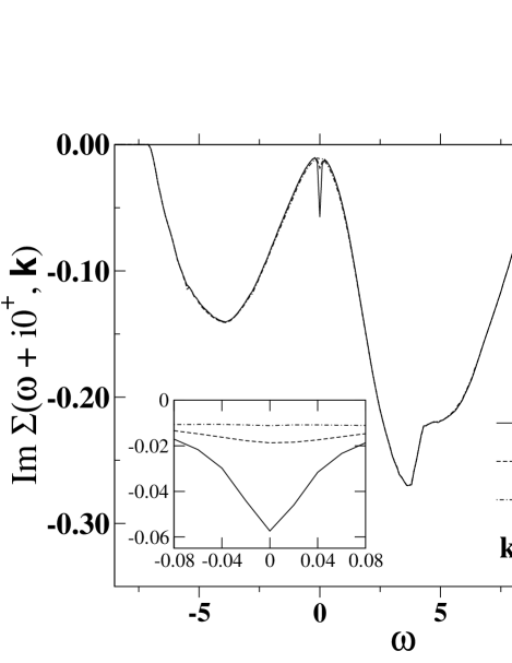
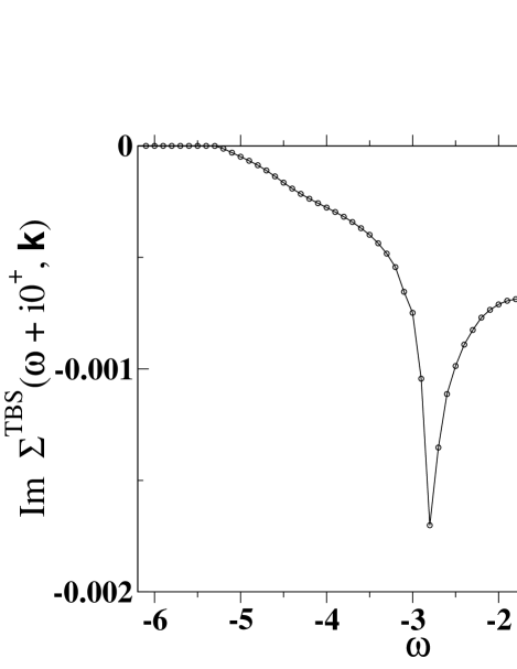
FIG. 2.: Self-energy at $U=-1.728$ for ${\mathbf{k}}=(k_{F},0)$ and different temperatures (left), and contribution from large ${\mathbf{q}}$ two-particle bound states for $\tau_{r}=0.01$ (right).

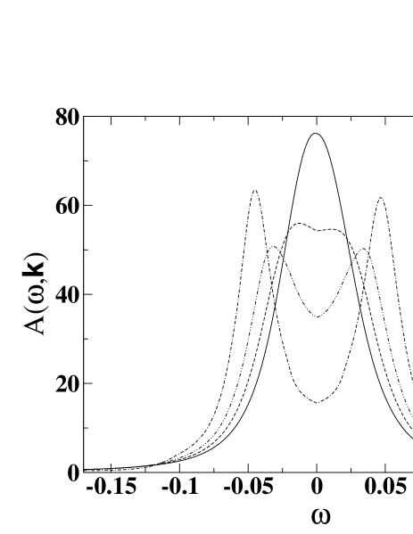
FIG. 3.: One-particle spectral function $A(\omega,{\mathbf{k}})$ at ${\mathbf{k}}=(k_{F},0)$ for $U=-1.728$ ($T_{c}=0.05$) and different values of the reduced temperature $\tau_{r}$.

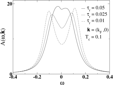
FIG. 4.: One-particle spectral function $A(\omega,{\mathbf{k}})$ at ${\mathbf{k}}=(k_{F},0)$ for $U=-2.034$ ($T_{c}=0.1$) and different values of the reduced temperature $\tau_{r}$.

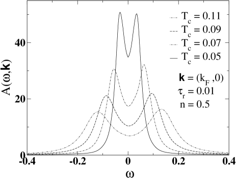
FIG. 5.: One-particle spectral function $A(\omega,{\mathbf{k}})$ at ${\mathbf{k}}=(k_{F},0)$ for different coupling strengths (i.e. various $T_{c}$) and fixed reduced temperature $\tau_{r}=0.01$.

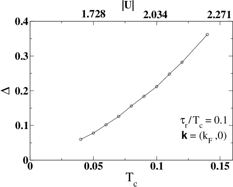
FIG. 6.: Size of the pseudogap as a function of $T_{c}$ for fixed ratio $\tau_{r}/T_{c}=0.1$ at ${\mathbf{k}}=(k_{F},0)$.

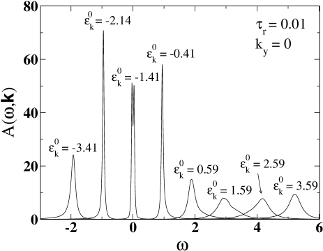
FIG. 7.: One-particle spectral function $A(\omega,{\mathbf{k}})$ for $U=-1.728$ ($T_{c}=0.05$) and $\tau_{r}=0.01$ for various wave vectors along the $k_{x}$-axis.

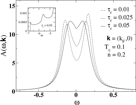
FIG. 8.: One-particle spectral function $A(\omega,{\mathbf{k}})$ at ${\mathbf{k}}=(k_{F},0)$ for $U=-2.667$ ($T_{c}=0.1$) and different values of the reduced temperature $\tau_{r}$; the density is $n=0.2$ here. The inset shows the tiny peak in the negative frequency tail of $A(\omega,{\mathbf{k}})$ caused by large-${\mathbf{q}}$ bound states.

FIG. 9.: Integration contour used to derive equation (A10).

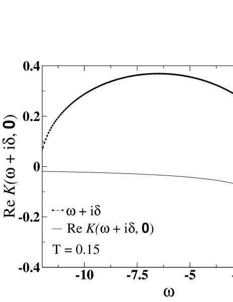
FIG. 10.: Zeros of the imaginary part of the pair propagator at $z=\omega+i\delta$ in the complex plane (upper curve) and real part of the pair propagator at these points (lower curve) for ${\mathbf{q}}=0$ and $T=0.15$.

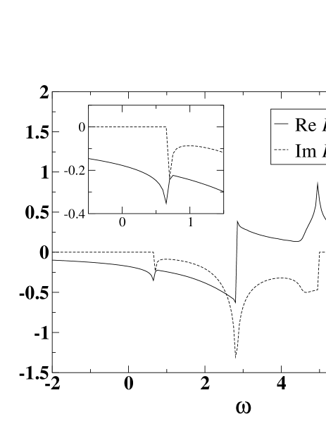
FIG. 11.: Frequency dependence of the pair propagator for ${\mathbf{q}}=(2.6,2.6)$ at $T=0.1$.

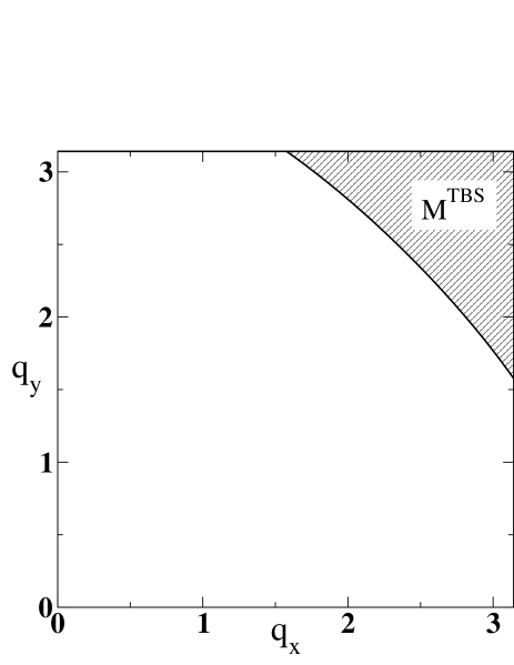
FIG. 12.: Domain $\text{M}^{\text{TBS}}$ in which two-particle bound states exist (for quarter-filling).

REFERENCES

- [1] Physical Properties of High Temperature Superconductors, edited by D.M. Ginsberg (World Scientific, Singapore, 1996).
- [2] For a review on pseudogaps in the normal phase of high temperature superconductors, see M. Randeria in Proceedings of the International School of Physics “Enrico Fermi”, edited by G. Iadonisi, J.R. Schrieffer and M.L. Chiofalo (IOS Press, Amsterdam, 1998), cond-mat 9710223.
- [3] For an early review on properties of the attractive Hubbard model (and extensions) see R. Micnas, J. Ranninger, and S. Robaszkiewicz, Rev. Mod. Phys. 62, 113 (1990).
- [4] M. Randeria, N. Trivedi, A. Moreo, and R.T. Scalettar, Phys. Rev. Lett. 69, 2001 (1992); N. Trivedi and M. Randeria, ibid 75, 312 (1995).
- [5] J.M. Singer, M.H. Pedersen, T. Schneider, H. Beck, and H.-G. Matuttis, Phys. Rev. B 54, 1286 (1996).
- [6] J.M. Singer, T. Schneider, and P.F. Meier, Eur. Phys. J. B 7, 37 (1999).
- [7] Y.M. Vilk, S. Allen, H. Touchette, S. Moukouri, L. Chen, and A.-M.S. Tremblay, J. Phys. Chem. Solids 59, 1873 (1998).
- [8] S. Allen, H. Touchette, S. Moukouri, Y.M. Vilk, and A.-M.S. Tremblay, Phys. Rev. Lett. 83, 4128 (1999).
- [9] B. Kyung, E.G. Klepfish, and P.E. Kornilovitch, Phys. Rev. Lett. 80, 3109 (1998); P.E. Kornilovitch and B. Kyung, J. Phys. Cond. Mat. 11, 741 (1999).
- [10] S. Schmitt-Rink, C.M. Varma, and A.E. Ruckenstein, Phys. Rev. Lett. 63, 445 (1989).
- [11] R. Micnas, M.H. Pedersen, S. Schafroth, T. Schneider, J.J. Rodriguez-Núñez, and H. Beck, Phys. Rev. B 52, 16223 (1995).
- [12] R. Frésard, B. Glaser, and P. Wölfle, J. Phys.: Condens. Matter 4, 8565 (1992).
- [13] M. Capezzali and H. Beck, Physica C 317-318, 482 (1999).
- [14] J. Schmalian, M. Langer, S. Grabowski, and K.H. Bennemann, Comp. Phys. Commun. 93, 141 (1996).
- [15] D.J. Thouless, Ann. Phys. 10, 553 (1960).
- [16] M. Randeria, Ji-Min Duan, and Lih-Yir Shieh, Phys. Rev. Lett. 62, 981 (1989).
- [17] H. Fukuyama, Y. Hasegawa, and O. Narikiyo, J. Phys. Soc. Jpn. 60, 2013 (1991).
- [18] J.W. Serene, Phys. Rev. B 40, 10873 (1989).
- [19] B. Kyung, S. Allen, and A.-M.S. Tremblay, condmat/0010001.
- [20] See, for example, B. Jankó, J. Maly, and K. Levin, Phys. Rev. B 56, 11407 (1997).
- [21] M. Keller, W. Metzner, U. Schollwöck, condmat/0101047.
- [22] S. Allen and A.-M.S. Tremblay, condmat/0010039.
- [23] D. Zanchi and H.J. Schulz, Phys. Rev. B 61, 13609 (2000); C.J. Halboth and W. Metzner, Phys. Rev. B 61, 7364 (2000); C. Honerkamp, M. Salmhofer, N. Furukawa, and T.M. Rice, Phys. Rev. B 63, 035109 (2001).