Level and Eigenfunction Statistics in Billiards with Surface Scattering

Abstract

Statistical properties of billiards with diffusive boundary scattering are investigated by means of the supersymmetric $\sigma$-model in a formulation appropriate for chaotic ballistic systems. We study level statistics, parametric level statistics, and properties of electron wavefunctions. In the universal regime, our results reproduce conclusions of the random matrix theory, while beyond this regime we obtain a variety of system-specific results determined by the classical dynamics in the billiard. Most notably, we find that level correlations do not vanish at arbitrary separation between energy levels, or if measured at arbitrarily large difference of magnetic fields. Saturation of the level number variance indicates strong rigidity of the spectrum. To study spatial correlations of wavefunction amplitudes, we reanalyze and refine derivation of the ballistic version of the $\sigma$-model. This allows us to obtain a proper matching of universal short-scale correlations with system-specific ones.

I Introduction

Chaotic cavities, commonly understood as quantum systems whose classical analogues exhibit chaotic dynamics, have become a common object of research in condensed matter physics. Experimentally, features of chaotic motion appear, among others, in quantum dots [2], microwave cavities [3], and small metallic clusters [4]. For definiteness, we talk below about electrons in quantum dots (billiards).

On the theoretical side, properties of chaotic cavities are subdivided into universal and non-universal. By universal we mean physical quantities which only depend on the global symmetry of the system (like the time reversibility) and possibly trivially scale with the size of the system, but are not influenced by any cavity-specific details of dynamics of the electron motion. At the same time, these quantities differ for systems with chaotic and integrable classical analogues, and are therefore conceptually important when one discusses signatures of chaotic behavior in quantum systems. Examples of universal effects include low-frequency level statistics, leading order conductance and shot noise. These properties are by now well understood and described by various types of random matrix theory (Gaussian ensembles of Hamiltonians for closed or almost closed systems or circular ensembles of scattering matrices for open systems).

On the other hand, non-universal quantities, such as, for instance, level correlation function for high energy separation or eigenfunction correlations at large distances, are determined by sample-specific details of electron motion. These non-universal quantities thus discriminate between the behavior of individual billiards.

A standard tool for treating fluctuations of the density of states (DOS) in chaotic systems is the real space path integral approach. Within this method, the DOS correlation function is given by Gutzwiller’s trace formula [5, 6] which has a form of a sum over periodic orbits of a specific billiard. To evaluate the formula explicitly in the non-universal regime, one has to resort to numerical treatment.

In this paper we will use an alternative approach which has attracted considerable interest recently, the ballistic $\sigma$-model. It generalizes the supersymmetric $\sigma$-model, which proved to be very successful for disordered metals [7, 8], to ballistic disordered systems [9, 10]. In the framework of this approach, all non-universal quantities are expressed through eigenvalues and eigenfunctions of the Liouville operator, which introduces non-universality. It has also been conjectured that the same $\sigma$-model in the limit of vanishing disorder describes statistical properties of spectra of individual classically chaotic system. This conjecture was further developed in Refs. [11, 12, 13] where the $\sigma$-model was obtained by means of energy averaging, and the Liouville operator was replaced by its regularization — the Perron-Frobenius operator. The progress along this direction is complicated by the fact that the eigenvalues of the Perron-Frobenius operator for many systems are unknown, while its eigenfunctions can be extremely singular.

We thus conclude that it is highly desirable to have an example of a chaotic system which is analytically solvable. We would expect that universal properties of such an example will conform with the predictions of the random matrix theory (RMT), whereas explicit expressions for non-universal quantities would improve our understanding of properties of chaotic cavities.

Currently, we are unaware of such an example with chaotic dynamics. However, one can instead treat systems with surface disorder, which leads to diffusive scattering at the boundary of a billiard. This model mimics the behavior of a system in the hard chaos regime: as a result of surface disorder any two arbitrary close trajectories spread apart after the first collision with the surface. This must be contrasted with slightly distorted integrable billiard with the typical spatial scale of this distortion being of the same order as the size of the system[14, 15, 16, 17]. Those systems, termed by the authors rough billiards, exhibit slow diffusion over angular momentum. Systems with surface disorder are also different from integrable systems with bulk disorder in the ballistic regime [18, 19, 20].

Studies of level and eigenfunction statistics [21, 22] have shown that, indeed, universal properties of a billiard with diffusive surface scattering agree with the RMT predictions. At the same time, non-universal features have been found which reflect the classical ballistic dynamics in the billiard. Subsequently, analytical results for persistent currents [23] and transport properties [24] of chaotic cavities have been obtained in the same model. Numerically, billiards with surface disorder have been studied in connection with the level [25, 26] and eigenfunction [25, 27] statistics, and magnetoconductance [28]. To this end, Refs. [25, 26, 27, 28] consider a lattice model with the boundary cites having random energies. A treatment of Ref. [29], which models surface disorder by cutting off the boundary cites by confining potential, and eventually proceeds with numerical evaluation of persistent currents, seems to describe a similar physical situation.

In this article, we perform a systematic analytical study of a circular billiard with boundary disorder, based on the $\sigma$-model approach. The paper is organized as follows. Section II presents the $\sigma$-model for a circular billiard with diffusive boundary scattering. We subsequently use this approach to derive the results for level statistics (Section III), parametric level statistics describing variation of individual energy levels with applied magnetic field (Section IV), and eigenfunction correlations (Section V). In Section VI we generalize the problem, imposing the mixed boundary condition, instead of purely diffusive reflection. This boundary condition enables us to model a broader class of chaotic systems, where the lowest Lyapunov exponent is parametrically different form the inverse time of flight. The obtained results are summarized in Section VII, where we also present a discussion of some open problems. A brief account of the results of Sections III and V has been previously given in Ref. [22]; the level statistics (Section III) were independently studied in Ref. [21].

II Circular billiard with diffusive boundary scattering: $\sigma$-model approach

A General considerations

We consider a $2D$ circular billiard of a radius $R$, which is clean (ballistic) inside, and contains some disorder (to be specified below) at the boundary. Our starting point is the $\sigma$-model for ballistic disordered systems [9, 10]. The effective action for this model has the form

$$F[g(\mathchoice{{\hbox{\boldmath$\displaystyle r$}}}{{\hbox{\boldmath$\textstyle r$}}}{{\hbox{\boldmath$\scriptstyle r$}}}{{\hbox{\boldmath$\scriptscriptstyle r$}}},\mathchoice{{\hbox{\boldmath$\displaystyle n$}}}{{\hbox{\boldmath$\textstyle n$}}}{{\hbox{\boldmath$\scriptstyle n$}}}{{\hbox{\boldmath$\scriptscriptstyle n$}}})] = -\frac{\pi\nu}{2}\int d\mathchoice{{\hbox{\boldmath$\displaystyle r$}}}{{\hbox{\boldmath$\textstyle r$}}}{{\hbox{\boldmath$\scriptstyle r$}}}{{\hbox{\boldmath$\scriptscriptstyle r$}}}{\rm Str}\left[i\omega\Lambda\langle g(\mathchoice{{\hbox{\boldmath$\displaystyle r$}}}{{\hbox{\boldmath$\textstyle r$}}}{{\hbox{\boldmath$\scriptstyle r$}}}{{\hbox{\boldmath$\scriptscriptstyle r$}}})\rangle-\frac{1}{2\tau(\mathchoice{{\hbox{\boldmath$\displaystyle r$}}}{{\hbox{\boldmath$\textstyle r$}}}{{\hbox{\boldmath$\scriptstyle r$}}}{{\hbox{\boldmath$\scriptscriptstyle r$}}})}\langle g(\mathchoice{{\hbox{\boldmath$\displaystyle r$}}}{{\hbox{\boldmath$\textstyle r$}}}{{\hbox{\boldmath$\scriptstyle r$}}}{{\hbox{\boldmath$\scriptscriptstyle r$}}})\rangle^{2}\right.$$ (1)

$$- \left.2v_{F}\langle\Lambda T^{-1}\mathchoice{{\hbox{\boldmath$\displaystyle n$}}}{{\hbox{\boldmath$\textstyle n$}}}{{\hbox{\boldmath$\scriptstyle n$}}}{{\hbox{\boldmath$\scriptscriptstyle n$}}}\nabla T\rangle\right].$$ (2)

Here the semi-classical Green’s function $g(\mathchoice{{\hbox{\boldmath$\displaystyle r$}}}{{\hbox{\boldmath$\textstyle r$}}}{{\hbox{\boldmath$\scriptstyle r$}}}{{\hbox{\boldmath$\scriptscriptstyle r$}}},\mathchoice{{\hbox{\boldmath$\displaystyle n$}}}{{\hbox{\boldmath$\textstyle n$}}}{{\hbox{\boldmath$\scriptstyle n$}}}{{\hbox{\boldmath$\scriptscriptstyle n$}}})$ integrated over energies is a $4\times 4$ supermatrix which depends on the coordinate $\textstyle r$ and direction of the momentum $\textstyle n$. To simplify the presentation we consider the case when the time-reversal symmetry is broken in the quantum problem but is preserved in the classical one, which can be achieved e.g. by applying a weak magnetic field. (See discussion in Section IV C). The angular brackets denote averaging over $\textstyle n$: $\langle{\cal O}(\mathchoice{{\hbox{\boldmath$\displaystyle n$}}}{{\hbox{\boldmath$\textstyle n$}}}{{\hbox{\boldmath$\scriptstyle n$}}}{{\hbox{\boldmath$\scriptscriptstyle n$}}})\rangle=\int d{\mathchoice{{\hbox{\boldmath$\displaystyle n$}}}{{\hbox{\boldmath$\textstyle n$}}}{{\hbox{\boldmath$\scriptstyle n$}}}{{\hbox{\boldmath$\scriptscriptstyle n$}}}}{\cal O}(\mathchoice{{\hbox{\boldmath$\displaystyle n$}}}{{\hbox{\boldmath$\textstyle n$}}}{{\hbox{\boldmath$\scriptstyle n$}}}{{\hbox{\boldmath$\scriptscriptstyle n$}}})$ with the normalization $\int d{\mathchoice{{\hbox{\boldmath$\displaystyle n$}}}{{\hbox{\boldmath$\textstyle n$}}}{{\hbox{\boldmath$\scriptstyle n$}}}{{\hbox{\boldmath$\scriptscriptstyle n$}}}}=1$, and the supertrace is defined as trace of boson-boson block minus trace of fermion-fermion one. The matrix $g$ is constrained by the condition $g(\mathchoice{{\hbox{\boldmath$\displaystyle r$}}}{{\hbox{\boldmath$\textstyle r$}}}{{\hbox{\boldmath$\scriptstyle r$}}}{{\hbox{\boldmath$\scriptscriptstyle r$}}},\mathchoice{{\hbox{\boldmath$\displaystyle n$}}}{{\hbox{\boldmath$\textstyle n$}}}{{\hbox{\boldmath$\scriptstyle n$}}}{{\hbox{\boldmath$\scriptscriptstyle n$}}})^{2}=1$, and generally can be represented as $g=T\Lambda T^{-1}$, with the matrix $\Lambda={\rm diag}(1,1,-1,-1)$ discriminating between retarded and advanced components of the Green’s function. As usual, $v_{F}$ and $\nu=m/(2\pi)$ denote the Fermi velocity and the density of states at the Fermi surface, respectively; $\tau(\mathchoice{{\hbox{\boldmath$\displaystyle r$}}}{{\hbox{\boldmath$\textstyle r$}}}{{\hbox{\boldmath$\scriptstyle r$}}}{{\hbox{\boldmath$\scriptscriptstyle r$}}})$ is the (position dependent) elastic scattering time, which originates from the disorder. We use the units with $\hbar=1$ in the rest of the paper.

When all the disorder is at the boundary the scattering time $\tau(\mathchoice{{\hbox{\boldmath$\displaystyle r$}}}{{\hbox{\boldmath$\textstyle r$}}}{{\hbox{\boldmath$\scriptstyle r$}}}{{\hbox{\boldmath$\scriptscriptstyle r$}}})$ must be chosen in a way that it is infinite everywhere except for a thin layer around the boundary. In the consideration below this term only modifies the boundary condition.

The action (1) differs from that in the $\sigma$-model for diffusive systems [7] in two respects: First, the Green’s function $g$ is defined in phase space; second, Eq. (1) is linear in gradients, whereas its diffusive counterpart is of second order in spatial derivatives. Despite this difference, methods developed for the calculation of level and eigenfunction statistics in diffusive systems can be applied here. Indeed, these properties are governed by the structure of the action in the vicinity of the homogeneous configuration of the $g$-field[30], $g(\mathchoice{{\hbox{\boldmath$\displaystyle r$}}}{{\hbox{\boldmath$\textstyle r$}}}{{\hbox{\boldmath$\scriptstyle r$}}}{{\hbox{\boldmath$\scriptscriptstyle r$}}},\mathchoice{{\hbox{\boldmath$\displaystyle n$}}}{{\hbox{\boldmath$\textstyle n$}}}{{\hbox{\boldmath$\scriptstyle n$}}}{{\hbox{\boldmath$\scriptscriptstyle n$}}})=\Lambda$ (see Refs. [7, 8] for review). In this case the action may be considerably simplified. Writing $T=1-W/2+\ldots$, we find the action to leading order in $W$,

$$F_{0}[W]=\frac{\pi\nu}{2}\int d\mathchoice{{\hbox{\boldmath$\displaystyle r$}}}{{\hbox{\boldmath$\textstyle r$}}}{{\hbox{\boldmath$\scriptstyle r$}}}{{\hbox{\boldmath$\scriptscriptstyle r$}}}d\mathchoice{{\hbox{\boldmath$\displaystyle n$}}}{{\hbox{\boldmath$\textstyle n$}}}{{\hbox{\boldmath$\scriptstyle n$}}}{{\hbox{\boldmath$\scriptscriptstyle n$}}}{\rm Str}\left[W_{21}\left(\hat{K}-i\omega\right)W_{12}\right],$$ (3)

where the indices $1,2$ refer to the “advanced-retarded” decomposition of $W$, and $\hat{K}\equiv v_{F}\mathchoice{{\hbox{\boldmath$\displaystyle n$}}}{{\hbox{\boldmath$\textstyle n$}}}{{\hbox{\boldmath$\scriptstyle n$}}}{{\hbox{\boldmath$\scriptscriptstyle n$}}}\nabla$ is the Liouville operator. This “linearized” action has now the same form as that of a diffusive system, with the diffusion operator $-D\nabla^{2}$ replaced by the Liouville operator. Thus, all the results derived previously from the linearized action for diffusive systems can be directly used for our model, provided the eigenvalues and eigenfunctions of the diffusion operator are replaced by those of the operator $\hat{K}$.

Since disorder is only present in the close vicinity of the boundary, we model it by supplementing the Liouville operator $\hat{K}$ by a boundary condition. Generally, the boundary condition for an eigenfunction $\varphi(\mathchoice{{\hbox{\boldmath$\displaystyle r$}}}{{\hbox{\boldmath$\textstyle r$}}}{{\hbox{\boldmath$\scriptstyle r$}}}{{\hbox{\boldmath$\scriptscriptstyle r$}}},\mathchoice{{\hbox{\boldmath$\displaystyle n$}}}{{\hbox{\boldmath$\textstyle n$}}}{{\hbox{\boldmath$\scriptstyle n$}}}{{\hbox{\boldmath$\scriptscriptstyle n$}}})$ relates its values for outgoing and incoming particles at a point on the surface,

$$\varphi(\mathchoice{{\hbox{\boldmath$\displaystyle r$}}}{{\hbox{\boldmath$\textstyle r$}}}{{\hbox{\boldmath$\scriptstyle r$}}}{{\hbox{\boldmath$\scriptscriptstyle r$}}},\mathchoice{{\hbox{\boldmath$\displaystyle n$}}}{{\hbox{\boldmath$\textstyle n$}}}{{\hbox{\boldmath$\scriptstyle n$}}}{{\hbox{\boldmath$\scriptscriptstyle n$}}}) = \left(\int_{(\mathchoice{{\hbox{\boldmath$\displaystyle N$}}}{{\hbox{\boldmath$\textstyle N$}}}{{\hbox{\boldmath$\scriptstyle N$}}}{{\hbox{\boldmath$\scriptscriptstyle N$}}}\mathchoice{{\hbox{\boldmath$\displaystyle n^{\prime}$}}}{{\hbox{\boldmath$\textstyle n^{\prime}$}}}{{\hbox{\boldmath$\scriptstyle n^{\prime}$}}}{{\hbox{\boldmath$\scriptscriptstyle n^{\prime}$}}})>0}\left(\mathchoice{{\hbox{\boldmath$\displaystyle N$}}}{{\hbox{\boldmath$\textstyle N$}}}{{\hbox{\boldmath$\scriptstyle N$}}}{{\hbox{\boldmath$\scriptscriptstyle N$}}}\mathchoice{{\hbox{\boldmath$\displaystyle n^{\prime}$}}}{{\hbox{\boldmath$\textstyle n^{\prime}$}}}{{\hbox{\boldmath$\scriptstyle n^{\prime}$}}}{{\hbox{\boldmath$\scriptscriptstyle n^{\prime}$}}}\right)B(\mathchoice{{\hbox{\boldmath$\displaystyle n$}}}{{\hbox{\boldmath$\textstyle n$}}}{{\hbox{\boldmath$\scriptstyle n$}}}{{\hbox{\boldmath$\scriptscriptstyle n$}}},\mathchoice{{\hbox{\boldmath$\displaystyle n$}}}{{\hbox{\boldmath$\textstyle n$}}}{{\hbox{\boldmath$\scriptstyle n$}}}{{\hbox{\boldmath$\scriptscriptstyle n$}}}^{\prime})d\mathchoice{{\hbox{\boldmath$\displaystyle n^{\prime}$}}}{{\hbox{\boldmath$\textstyle n^{\prime}$}}}{{\hbox{\boldmath$\scriptstyle n^{\prime}$}}}{{\hbox{\boldmath$\scriptscriptstyle n^{\prime}$}}}\right)^{-1}$$ (4)

$$\times \int_{(\mathchoice{{\hbox{\boldmath$\displaystyle N$}}}{{\hbox{\boldmath$\textstyle N$}}}{{\hbox{\boldmath$\scriptstyle N$}}}{{\hbox{\boldmath$\scriptscriptstyle N$}}}\mathchoice{{\hbox{\boldmath$\displaystyle n^{\prime}$}}}{{\hbox{\boldmath$\textstyle n^{\prime}$}}}{{\hbox{\boldmath$\scriptstyle n^{\prime}$}}}{{\hbox{\boldmath$\scriptscriptstyle n^{\prime}$}}})>0}\left(\mathchoice{{\hbox{\boldmath$\displaystyle N$}}}{{\hbox{\boldmath$\textstyle N$}}}{{\hbox{\boldmath$\scriptstyle N$}}}{{\hbox{\boldmath$\scriptscriptstyle N$}}}\mathchoice{{\hbox{\boldmath$\displaystyle n^{\prime}$}}}{{\hbox{\boldmath$\textstyle n^{\prime}$}}}{{\hbox{\boldmath$\scriptstyle n^{\prime}$}}}{{\hbox{\boldmath$\scriptscriptstyle n^{\prime}$}}}\right)B(\mathchoice{{\hbox{\boldmath$\displaystyle n$}}}{{\hbox{\boldmath$\textstyle n$}}}{{\hbox{\boldmath$\scriptstyle n$}}}{{\hbox{\boldmath$\scriptscriptstyle n$}}},\mathchoice{{\hbox{\boldmath$\displaystyle n$}}}{{\hbox{\boldmath$\textstyle n$}}}{{\hbox{\boldmath$\scriptstyle n$}}}{{\hbox{\boldmath$\scriptscriptstyle n$}}}^{\prime})\varphi(\mathchoice{{\hbox{\boldmath$\displaystyle r$}}}{{\hbox{\boldmath$\textstyle r$}}}{{\hbox{\boldmath$\scriptstyle r$}}}{{\hbox{\boldmath$\scriptscriptstyle r$}}},\mathchoice{{\hbox{\boldmath$\displaystyle n^{\prime}$}}}{{\hbox{\boldmath$\textstyle n^{\prime}$}}}{{\hbox{\boldmath$\scriptstyle n^{\prime}$}}}{{\hbox{\boldmath$\scriptscriptstyle n^{\prime}$}}})d\mathchoice{{\hbox{\boldmath$\displaystyle n^{\prime}$}}}{{\hbox{\boldmath$\textstyle n^{\prime}$}}}{{\hbox{\boldmath$\scriptstyle n^{\prime}$}}}{{\hbox{\boldmath$\scriptscriptstyle n^{\prime}$}}},$$ (6)

$$\hskip 113.81102pt\left(\mathchoice{{\hbox{\boldmath$\displaystyle N$}}}{{\hbox{\boldmath$\textstyle N$}}}{{\hbox{\boldmath$\scriptstyle N$}}}{{\hbox{\boldmath$\scriptscriptstyle N$}}}\mathchoice{{\hbox{\boldmath$\displaystyle n$}}}{{\hbox{\boldmath$\textstyle n$}}}{{\hbox{\boldmath$\scriptstyle n$}}}{{\hbox{\boldmath$\scriptscriptstyle n$}}}\right)<0,$$

with some kernel $B$. Here the point $\textstyle r$ is taken at the surface, $|r|=R$, and $\textstyle N$ is an outward normal to the boundary. The form (4) ensures that no current flows through the boundary of the billiard.

The scattering kernel $B$ was intensively studied in the context of the boundary condition for the distribution function (for review, see Ref. [31]) and found to be model dependent. Realistic models of short-range surface randomness (like a boundary narrow layer of impurities, or a ballistic orifice in a disordered medium) lead to general boundary conditions of the type (4), where the kernel $B$ is a parameterless function of order one.

Following Refs. [32, 33, 34], we approximate the above, rather complicated, boundary condition by a simpler one, where an electron reflects diffusively with probability $\alpha$ and specularly with probability $1-\alpha$ ($0\leq\alpha\leq 1$),

$$\varphi(\mathchoice{{\hbox{\boldmath$\displaystyle r$}}}{{\hbox{\boldmath$\textstyle r$}}}{{\hbox{\boldmath$\scriptstyle r$}}}{{\hbox{\boldmath$\scriptscriptstyle r$}}},\mathchoice{{\hbox{\boldmath$\displaystyle n$}}}{{\hbox{\boldmath$\textstyle n$}}}{{\hbox{\boldmath$\scriptstyle n$}}}{{\hbox{\boldmath$\scriptscriptstyle n$}}}) = \pi\alpha\int_{(\mathchoice{{\hbox{\boldmath$\displaystyle N$}}}{{\hbox{\boldmath$\textstyle N$}}}{{\hbox{\boldmath$\scriptstyle N$}}}{{\hbox{\boldmath$\scriptscriptstyle N$}}}\mathchoice{{\hbox{\boldmath$\displaystyle n^{\prime}$}}}{{\hbox{\boldmath$\textstyle n^{\prime}$}}}{{\hbox{\boldmath$\scriptstyle n^{\prime}$}}}{{\hbox{\boldmath$\scriptscriptstyle n^{\prime}$}}})>0}\left(\mathchoice{{\hbox{\boldmath$\displaystyle N$}}}{{\hbox{\boldmath$\textstyle N$}}}{{\hbox{\boldmath$\scriptstyle N$}}}{{\hbox{\boldmath$\scriptscriptstyle N$}}}\mathchoice{{\hbox{\boldmath$\displaystyle n^{\prime}$}}}{{\hbox{\boldmath$\textstyle n^{\prime}$}}}{{\hbox{\boldmath$\scriptstyle n^{\prime}$}}}{{\hbox{\boldmath$\scriptscriptstyle n^{\prime}$}}}\right)\varphi(\mathchoice{{\hbox{\boldmath$\displaystyle r$}}}{{\hbox{\boldmath$\textstyle r$}}}{{\hbox{\boldmath$\scriptstyle r$}}}{{\hbox{\boldmath$\scriptscriptstyle r$}}},\mathchoice{{\hbox{\boldmath$\displaystyle n^{\prime}$}}}{{\hbox{\boldmath$\textstyle n^{\prime}$}}}{{\hbox{\boldmath$\scriptstyle n^{\prime}$}}}{{\hbox{\boldmath$\scriptscriptstyle n^{\prime}$}}})d\mathchoice{{\hbox{\boldmath$\displaystyle n^{\prime}$}}}{{\hbox{\boldmath$\textstyle n^{\prime}$}}}{{\hbox{\boldmath$\scriptstyle n^{\prime}$}}}{{\hbox{\boldmath$\scriptscriptstyle n^{\prime}$}}}$$ (7)

$$+ (1-\alpha)\varphi(\mathchoice{{\hbox{\boldmath$\displaystyle r$}}}{{\hbox{\boldmath$\textstyle r$}}}{{\hbox{\boldmath$\scriptstyle r$}}}{{\hbox{\boldmath$\scriptscriptstyle r$}}},\mathchoice{{\hbox{\boldmath$\displaystyle n^{\prime\prime}$}}}{{\hbox{\boldmath$\textstyle n^{\prime\prime}$}}}{{\hbox{\boldmath$\scriptstyle n^{\prime\prime}$}}}{{\hbox{\boldmath$\scriptscriptstyle n^{\prime\prime}$}}}),\ \ \ \ \ \left(\mathchoice{{\hbox{\boldmath$\displaystyle N$}}}{{\hbox{\boldmath$\textstyle N$}}}{{\hbox{\boldmath$\scriptstyle N$}}}{{\hbox{\boldmath$\scriptscriptstyle N$}}}\mathchoice{{\hbox{\boldmath$\displaystyle n$}}}{{\hbox{\boldmath$\textstyle n$}}}{{\hbox{\boldmath$\scriptstyle n$}}}{{\hbox{\boldmath$\scriptscriptstyle n$}}}\right)<0,$$ (8)

where the vector $\textstyle n^{\prime\prime}$ is chosen so that the reflection from $\textstyle n^{\prime\prime}$ to $\textstyle n$ is purely specular. Although Eq. (7) does not correspond to any particular known microscopic model of disorder, it is commonly believed to provide a good qualitative description of surface scattering interpolating between purely diffusive ($\alpha=1$) and purely specular ($\alpha=0$) reflection.

With the exception of Section VI, we consider below purely diffusive reflection (Eq. (7) with $\alpha=1$). Physically, it describes quantum scattering due to short-range disorder (correlated at the scale of the order of the wavelength $2\pi/p_{F}$). Alternatively, the diffusive boundary condition of this type may result from the purely classical scattering off a strongly corrugated surface. As noted in the Introduction, atomic-scale disorder has the feature that an electron loses the memory about the direction of previous motion after the first collision with the boundary. The system is thus described by two characteristic energies, which are the mean level spacing $\Delta$ and the inverse time of flight through the billiard $v_{F}/R$. This is a special type of a billiard, analogous to “hard chaos” behavior of genuinely chaotic systems.

Section VI is devoted to the general situation $\alpha<1$. A new regime appears for $\alpha\ll 1$ when the time $R/(v_{F}\alpha)$ during which an electron remembers its initial direction of motion differs parametrically from the time of flight $R/v_{F}$. In this regime the system is described by three distinct energy scales.

B Eigenvalues of the Liouville operator for diffusive scattering

As we have mentioned, the level statistics of our billiard are entirely determined by the eigenvalues of the Liouville operator $\hat{K}$. Due to the boundary condition (7) the evolution becomes irreversible, the eigenvalues of $\hat{K}$ have positive real part, and no regularization, like that discussed in Refs. [12, 13] is needed. Below we review properties of eigenvalues $\lambda$ of the operator $\hat{K}$,

$$v_{F}\mathchoice{{\hbox{\boldmath$\displaystyle n$}}}{{\hbox{\boldmath$\textstyle n$}}}{{\hbox{\boldmath$\scriptstyle n$}}}{{\hbox{\boldmath$\scriptscriptstyle n$}}}\nabla\varphi_{\lambda}(\mathchoice{{\hbox{\boldmath$\displaystyle r$}}}{{\hbox{\boldmath$\textstyle r$}}}{{\hbox{\boldmath$\scriptstyle r$}}}{{\hbox{\boldmath$\scriptscriptstyle r$}}},\mathchoice{{\hbox{\boldmath$\displaystyle n$}}}{{\hbox{\boldmath$\textstyle n$}}}{{\hbox{\boldmath$\scriptstyle n$}}}{{\hbox{\boldmath$\scriptscriptstyle n$}}})=\lambda\varphi_{\lambda}(\mathchoice{{\hbox{\boldmath$\displaystyle r$}}}{{\hbox{\boldmath$\textstyle r$}}}{{\hbox{\boldmath$\scriptstyle r$}}}{{\hbox{\boldmath$\scriptscriptstyle r$}}},\mathchoice{{\hbox{\boldmath$\displaystyle n$}}}{{\hbox{\boldmath$\textstyle n$}}}{{\hbox{\boldmath$\scriptstyle n$}}}{{\hbox{\boldmath$\scriptscriptstyle n$}}}),$$ (9)

supplemented by the boundary condition

FIG. 1.: Natural parameterization of the constant energy shell in terms of position $\mathchoice{{\hbox{\boldmath$\displaystyle r$}}}{{\hbox{\boldmath$\textstyle r$}}}{{\hbox{\boldmath$\scriptstyle r$}}}{{\hbox{\boldmath$\scriptscriptstyle r$}}}=(r,\vartheta)$ and direction of motion $\textstyle n$ and its relation to the alternative parameterization by the coordinates $\theta,\theta^{\prime},x$ introduced in the text.

$$\varphi(\mathchoice{{\hbox{\boldmath$\displaystyle r$}}}{{\hbox{\boldmath$\textstyle r$}}}{{\hbox{\boldmath$\scriptstyle r$}}}{{\hbox{\boldmath$\scriptscriptstyle r$}}},\mathchoice{{\hbox{\boldmath$\displaystyle n$}}}{{\hbox{\boldmath$\textstyle n$}}}{{\hbox{\boldmath$\scriptstyle n$}}}{{\hbox{\boldmath$\scriptscriptstyle n$}}})=\pi\int_{(\mathchoice{{\hbox{\boldmath$\displaystyle N$}}}{{\hbox{\boldmath$\textstyle N$}}}{{\hbox{\boldmath$\scriptstyle N$}}}{{\hbox{\boldmath$\scriptscriptstyle N$}}}\mathchoice{{\hbox{\boldmath$\displaystyle n^{\prime}$}}}{{\hbox{\boldmath$\textstyle n^{\prime}$}}}{{\hbox{\boldmath$\scriptstyle n^{\prime}$}}}{{\hbox{\boldmath$\scriptscriptstyle n^{\prime}$}}})>0}\left(\mathchoice{{\hbox{\boldmath$\displaystyle N$}}}{{\hbox{\boldmath$\textstyle N$}}}{{\hbox{\boldmath$\scriptstyle N$}}}{{\hbox{\boldmath$\scriptscriptstyle N$}}}\mathchoice{{\hbox{\boldmath$\displaystyle n^{\prime}$}}}{{\hbox{\boldmath$\textstyle n^{\prime}$}}}{{\hbox{\boldmath$\scriptstyle n^{\prime}$}}}{{\hbox{\boldmath$\scriptscriptstyle n^{\prime}$}}}\right)\varphi(\mathchoice{{\hbox{\boldmath$\displaystyle r$}}}{{\hbox{\boldmath$\textstyle r$}}}{{\hbox{\boldmath$\scriptstyle r$}}}{{\hbox{\boldmath$\scriptscriptstyle r$}}},\mathchoice{{\hbox{\boldmath$\displaystyle n^{\prime}$}}}{{\hbox{\boldmath$\textstyle n^{\prime}$}}}{{\hbox{\boldmath$\scriptstyle n^{\prime}$}}}{{\hbox{\boldmath$\scriptscriptstyle n^{\prime}$}}})d\mathchoice{{\hbox{\boldmath$\displaystyle n^{\prime}$}}}{{\hbox{\boldmath$\textstyle n^{\prime}$}}}{{\hbox{\boldmath$\scriptstyle n^{\prime}$}}}{{\hbox{\boldmath$\scriptscriptstyle n^{\prime}$}}},\ \ \ \left(\mathchoice{{\hbox{\boldmath$\displaystyle N$}}}{{\hbox{\boldmath$\textstyle N$}}}{{\hbox{\boldmath$\scriptstyle N$}}}{{\hbox{\boldmath$\scriptscriptstyle N$}}}\mathchoice{{\hbox{\boldmath$\displaystyle n$}}}{{\hbox{\boldmath$\textstyle n$}}}{{\hbox{\boldmath$\scriptstyle n$}}}{{\hbox{\boldmath$\scriptscriptstyle n$}}}\right)<0.$$ (10)

The constant energy surface can be parameterized by the three real numbers $(\theta,\theta^{\prime},x)$, where the angle $\theta$ ($\theta^{\prime}$) corresponds to the point where the straight line passing through $\mathchoice{{\hbox{\boldmath$\displaystyle r$}}}{{\hbox{\boldmath$\textstyle r$}}}{{\hbox{\boldmath$\scriptstyle r$}}}{{\hbox{\boldmath$\scriptscriptstyle r$}}}=(r,\vartheta)$ in the direction $\textstyle n$ ($\textstyle-n$) crosses the boundary, and $x$ is the distance from the boundary to $\textstyle r$ along this straight line (see Fig. 1). To cover the whole energy surface the parameters must change in the region $0<\theta,\theta^{\prime}<2\pi$; $0<x<2R\sin|(\theta-\theta^{\prime})/2|$. Eq. (9) then expresses the eigenfunction $\varphi$ at any $x$ through the eigenfunction at $x=0$, i.e. through the function describing particles scattered from the boundary. In particular, the eigenfunction for the particles arriving to the boundary is

$$\varphi_{\lambda}\left(\theta,\theta^{\prime},x=2R\sin\left|\frac{\theta-\theta^{\prime}}{2}\right|\right)$$ (11)

$$=\varphi_{\lambda}\left(\theta,\theta^{\prime},x=0\right)\exp\left(\frac{2R\lambda}{v_{F}}\sin\left|\frac{\theta-\theta^{\prime}}{2}\right|\right).$$ (12)

Now the boundary condition (10) is used to find a closed integral equation for $\varphi_{\lambda}(\theta,\theta^{\prime},x=0)$ which is simplified by the Ansatz $\varphi_{\lambda}(\theta,\theta^{\prime},x=0)=\tilde{\varphi}(\theta-\theta^{\prime})\exp(il\theta^{\prime})$, $l$ having the meaning of the angular momentum,

$$\tilde{\varphi}(\theta)e^{-il\theta}=\frac{1}{2}\int_{0}^{\pi}d\tilde{\theta}\ \sin\tilde{\theta}e^{2\xi\sin\tilde{\theta}}\tilde{\varphi}(2\tilde{\theta}),$$ (13)

with the notation $\xi\equiv R\lambda/v_{F}$. Eq. (13) only has solutions for the eigenvalues which obey the following equation,

$$\tilde{J}_{l}(\xi)\equiv-1+\frac{1}{2}\int_{0}^{\pi}d\theta\ \sin\theta\exp\left[2il\theta+2\xi\sin\theta\right]=0.$$ (14)

The eigenvalue equation (14) can not be solved analytically in a closed form, however the combinations of eigenvalues which enter level statistics can be expressed through the function $\tilde{J}_{l}$. Below we list some properties of these eigenvalues.

FIG. 2.: The first $11\times 11$ ($0\leq k,l<11$) eigenvalues of the Liouville operator $\hat{K}$ in units of $v_{F}/R$, as given by roots of Eq. (14).

For each value of $l=0,\pm 1,\pm 2,\ldots$ Eq.(14) has a set of solutions $\xi_{lk}$ with $\xi_{lk}=\xi_{-l,k}=\xi^{*}_{l,-k}$, which can be labeled with $k=0,\pm 1,\pm 2,\ldots$ (even $l$) or $k=\pm 1/2,\pm 3/2,\ldots$ (odd $l$). Thus, the eigenvalues form a two-parameter set. For $l=k=0$ we have $\xi_{00}=0$, corresponding to the zero mode $\varphi(\mathchoice{{\hbox{\boldmath$\displaystyle r$}}}{{\hbox{\boldmath$\textstyle r$}}}{{\hbox{\boldmath$\scriptstyle r$}}}{{\hbox{\boldmath$\scriptscriptstyle r$}}},\mathchoice{{\hbox{\boldmath$\displaystyle n$}}}{{\hbox{\boldmath$\textstyle n$}}}{{\hbox{\boldmath$\scriptstyle n$}}}{{\hbox{\boldmath$\scriptscriptstyle n$}}})=\mbox{const}$. All other eigenvalues have positive real part $\mbox{Re}\,\xi_{lk}>0$ and govern the relaxation of the corresponding classical system to the homogeneous distribution in the phase space.

The asymptotic form of the solutions of Eq.(14) for large $|k|$ and/or $|l|$ is given by the saddle-point method:

$$\xi_{kl}\approx\left\{\begin{array}[]{lr}0.66l+0.14\ln l+0.55\pi ik,&0\leq k\ll l\\ (\ln k)/4+\pi i(k+1/8),&0\leq l\ll k\end{array}\right..$$ (17)

Note that for $k=0$ all eigenvalues are real, while for high values of $k$ they lie close to the imaginary axis and do not depend on $l$. Fig. 2 shows a plot of the first 11$\times$11 eigenvalues of the operator $\hat{K}$.

C Green’s function of the Liouville operator

The Green’s function of the Liouville operator ${\cal D}(\mathchoice{{\hbox{\boldmath$\displaystyle r$}}}{{\hbox{\boldmath$\textstyle r$}}}{{\hbox{\boldmath$\scriptstyle r$}}}{{\hbox{\boldmath$\scriptscriptstyle r$}}}_{1},\mathchoice{{\hbox{\boldmath$\displaystyle n$}}}{{\hbox{\boldmath$\textstyle n$}}}{{\hbox{\boldmath$\scriptstyle n$}}}{{\hbox{\boldmath$\scriptscriptstyle n$}}}_{1};\mathchoice{{\hbox{\boldmath$\displaystyle r$}}}{{\hbox{\boldmath$\textstyle r$}}}{{\hbox{\boldmath$\scriptstyle r$}}}{{\hbox{\boldmath$\scriptscriptstyle r$}}}_{2},\mathchoice{{\hbox{\boldmath$\displaystyle n$}}}{{\hbox{\boldmath$\textstyle n$}}}{{\hbox{\boldmath$\scriptstyle n$}}}{{\hbox{\boldmath$\scriptscriptstyle n$}}}_{2})$ is the time-integrated probability to find the particle at the point of the phase space $(\mathchoice{{\hbox{\boldmath$\displaystyle r$}}}{{\hbox{\boldmath$\textstyle r$}}}{{\hbox{\boldmath$\scriptstyle r$}}}{{\hbox{\boldmath$\scriptscriptstyle r$}}}_{1},\mathchoice{{\hbox{\boldmath$\displaystyle n$}}}{{\hbox{\boldmath$\textstyle n$}}}{{\hbox{\boldmath$\scriptstyle n$}}}{{\hbox{\boldmath$\scriptscriptstyle n$}}}_{1})$ if it started the motion at $(\mathchoice{{\hbox{\boldmath$\displaystyle r$}}}{{\hbox{\boldmath$\textstyle r$}}}{{\hbox{\boldmath$\scriptstyle r$}}}{{\hbox{\boldmath$\scriptscriptstyle r$}}}_{2},\mathchoice{{\hbox{\boldmath$\displaystyle n$}}}{{\hbox{\boldmath$\textstyle n$}}}{{\hbox{\boldmath$\scriptstyle n$}}}{{\hbox{\boldmath$\scriptscriptstyle n$}}}_{2})$. This function obeys the equation

$$\hat{K}{\cal D}(\mathchoice{{\hbox{\boldmath$\displaystyle r$}}}{{\hbox{\boldmath$\textstyle r$}}}{{\hbox{\boldmath$\scriptstyle r$}}}{{\hbox{\boldmath$\scriptscriptstyle r$}}}_{1},\mathchoice{{\hbox{\boldmath$\displaystyle n$}}}{{\hbox{\boldmath$\textstyle n$}}}{{\hbox{\boldmath$\scriptstyle n$}}}{{\hbox{\boldmath$\scriptscriptstyle n$}}}_{1};\mathchoice{{\hbox{\boldmath$\displaystyle r$}}}{{\hbox{\boldmath$\textstyle r$}}}{{\hbox{\boldmath$\scriptstyle r$}}}{{\hbox{\boldmath$\scriptscriptstyle r$}}}_{2},\mathchoice{{\hbox{\boldmath$\displaystyle n$}}}{{\hbox{\boldmath$\textstyle n$}}}{{\hbox{\boldmath$\scriptstyle n$}}}{{\hbox{\boldmath$\scriptscriptstyle n$}}}_{2})=$$ (18)

$$\qquad\frac{1}{\pi\nu}\left[\delta(\mathchoice{{\hbox{\boldmath$\displaystyle r$}}}{{\hbox{\boldmath$\textstyle r$}}}{{\hbox{\boldmath$\scriptstyle r$}}}{{\hbox{\boldmath$\scriptscriptstyle r$}}}_{1}-\mathchoice{{\hbox{\boldmath$\displaystyle r$}}}{{\hbox{\boldmath$\textstyle r$}}}{{\hbox{\boldmath$\scriptstyle r$}}}{{\hbox{\boldmath$\scriptscriptstyle r$}}}_{2})\delta(\mathchoice{{\hbox{\boldmath$\displaystyle n$}}}{{\hbox{\boldmath$\textstyle n$}}}{{\hbox{\boldmath$\scriptstyle n$}}}{{\hbox{\boldmath$\scriptscriptstyle n$}}}_{1}-\mathchoice{{\hbox{\boldmath$\displaystyle n$}}}{{\hbox{\boldmath$\textstyle n$}}}{{\hbox{\boldmath$\scriptstyle n$}}}{{\hbox{\boldmath$\scriptscriptstyle n$}}}_{2})-\frac{1}{V}\right],$$ (19)

where $V=\pi R^{2}$ is the area of the billiard, and the operator $\hat{K}$ acts on the variables $\mathchoice{{\hbox{\boldmath$\displaystyle r$}}}{{\hbox{\boldmath$\textstyle r$}}}{{\hbox{\boldmath$\scriptstyle r$}}}{{\hbox{\boldmath$\scriptscriptstyle r$}}}_{1},\mathchoice{{\hbox{\boldmath$\displaystyle n$}}}{{\hbox{\boldmath$\textstyle n$}}}{{\hbox{\boldmath$\scriptstyle n$}}}{{\hbox{\boldmath$\scriptscriptstyle n$}}}_{1}$. The Green’s function is related to the correlation of the wavefunctions (Section V). It is also used in the alternative derivation of the low-energy level correlation function, see Section III B.

1 Green’s function integrated over momenta

In this subsection we calculate the Green’s function integrated over momenta:

$$\Pi_{B}(\mathchoice{{\hbox{\boldmath$\displaystyle r$}}}{{\hbox{\boldmath$\textstyle r$}}}{{\hbox{\boldmath$\scriptstyle r$}}}{{\hbox{\boldmath$\scriptscriptstyle r$}}}_{1},\mathchoice{{\hbox{\boldmath$\displaystyle r$}}}{{\hbox{\boldmath$\textstyle r$}}}{{\hbox{\boldmath$\scriptstyle r$}}}{{\hbox{\boldmath$\scriptscriptstyle r$}}}_{2})=\int d\mathchoice{{\hbox{\boldmath$\displaystyle n$}}}{{\hbox{\boldmath$\textstyle n$}}}{{\hbox{\boldmath$\scriptstyle n$}}}{{\hbox{\boldmath$\scriptscriptstyle n$}}}_{1}d\mathchoice{{\hbox{\boldmath$\displaystyle n$}}}{{\hbox{\boldmath$\textstyle n$}}}{{\hbox{\boldmath$\scriptstyle n$}}}{{\hbox{\boldmath$\scriptscriptstyle n$}}}_{2}{\cal D}(\mathchoice{{\hbox{\boldmath$\displaystyle r$}}}{{\hbox{\boldmath$\textstyle r$}}}{{\hbox{\boldmath$\scriptstyle r$}}}{{\hbox{\boldmath$\scriptscriptstyle r$}}}_{1},\mathchoice{{\hbox{\boldmath$\displaystyle n$}}}{{\hbox{\boldmath$\textstyle n$}}}{{\hbox{\boldmath$\scriptstyle n$}}}{{\hbox{\boldmath$\scriptscriptstyle n$}}}_{1};\mathchoice{{\hbox{\boldmath$\displaystyle r$}}}{{\hbox{\boldmath$\textstyle r$}}}{{\hbox{\boldmath$\scriptstyle r$}}}{{\hbox{\boldmath$\scriptscriptstyle r$}}}_{2},\mathchoice{{\hbox{\boldmath$\displaystyle n$}}}{{\hbox{\boldmath$\textstyle n$}}}{{\hbox{\boldmath$\scriptstyle n$}}}{{\hbox{\boldmath$\scriptscriptstyle n$}}}_{2}),$$ (20)

which describes the probability to find an electron at $\mathchoice{{\hbox{\boldmath$\displaystyle r$}}}{{\hbox{\boldmath$\textstyle r$}}}{{\hbox{\boldmath$\scriptstyle r$}}}{{\hbox{\boldmath$\scriptscriptstyle r$}}}_{1}$ after it has been found at $\mathchoice{{\hbox{\boldmath$\displaystyle r$}}}{{\hbox{\boldmath$\textstyle r$}}}{{\hbox{\boldmath$\scriptstyle r$}}}{{\hbox{\boldmath$\scriptscriptstyle r$}}}_{2}$, and is important for the wavefunction correlation. Integrating Eq. (18) over $d\mathchoice{{\hbox{\boldmath$\displaystyle n$}}}{{\hbox{\boldmath$\textstyle n$}}}{{\hbox{\boldmath$\scriptstyle n$}}}{{\hbox{\boldmath$\scriptscriptstyle n$}}}_{2}$, we obtain

$$v_{F}\mathchoice{{\hbox{\boldmath$\displaystyle n$}}}{{\hbox{\boldmath$\textstyle n$}}}{{\hbox{\boldmath$\scriptstyle n$}}}{{\hbox{\boldmath$\scriptscriptstyle n$}}}_{1}\frac{\partial h}{\partial{\mathchoice{{\hbox{\boldmath$\displaystyle r$}}}{{\hbox{\boldmath$\textstyle r$}}}{{\hbox{\boldmath$\scriptstyle r$}}}{{\hbox{\boldmath$\scriptscriptstyle r$}}}}_{1}}=\frac{1}{\pi\nu}\left[\delta(\mathchoice{{\hbox{\boldmath$\displaystyle r$}}}{{\hbox{\boldmath$\textstyle r$}}}{{\hbox{\boldmath$\scriptstyle r$}}}{{\hbox{\boldmath$\scriptscriptstyle r$}}}_{1}-\mathchoice{{\hbox{\boldmath$\displaystyle r$}}}{{\hbox{\boldmath$\textstyle r$}}}{{\hbox{\boldmath$\scriptstyle r$}}}{{\hbox{\boldmath$\scriptscriptstyle r$}}}_{2})-\frac{1}{V}\right],$$ (21)

where $h(\mathchoice{{\hbox{\boldmath$\displaystyle r$}}}{{\hbox{\boldmath$\textstyle r$}}}{{\hbox{\boldmath$\scriptstyle r$}}}{{\hbox{\boldmath$\scriptscriptstyle r$}}}_{1},\mathchoice{{\hbox{\boldmath$\displaystyle n$}}}{{\hbox{\boldmath$\textstyle n$}}}{{\hbox{\boldmath$\scriptstyle n$}}}{{\hbox{\boldmath$\scriptscriptstyle n$}}}_{1};\mathchoice{{\hbox{\boldmath$\displaystyle r$}}}{{\hbox{\boldmath$\textstyle r$}}}{{\hbox{\boldmath$\scriptstyle r$}}}{{\hbox{\boldmath$\scriptscriptstyle r$}}}_{2})=\int d\mathchoice{{\hbox{\boldmath$\displaystyle n$}}}{{\hbox{\boldmath$\textstyle n$}}}{{\hbox{\boldmath$\scriptstyle n$}}}{{\hbox{\boldmath$\scriptscriptstyle n$}}}_{2}{\cal D}$. To solve Eq. (21), we use the same strategy as with Eq. (9) and replace the coordinates $(\mathchoice{{\hbox{\boldmath$\displaystyle r$}}}{{\hbox{\boldmath$\textstyle r$}}}{{\hbox{\boldmath$\scriptstyle r$}}}{{\hbox{\boldmath$\scriptscriptstyle r$}}}_{1},\mathchoice{{\hbox{\boldmath$\displaystyle n$}}}{{\hbox{\boldmath$\textstyle n$}}}{{\hbox{\boldmath$\scriptstyle n$}}}{{\hbox{\boldmath$\scriptscriptstyle n$}}}_{1})$ by the variables $\theta_{1},\theta_{1}^{\prime},x_{1}$,

$$h(\theta_{1},\theta_{1}^{\prime},x_{1};\mathchoice{{\hbox{\boldmath$\displaystyle r$}}}{{\hbox{\boldmath$\textstyle r$}}}{{\hbox{\boldmath$\scriptstyle r$}}}{{\hbox{\boldmath$\scriptscriptstyle r$}}}_{2})=h(\theta_{1},\theta_{1}^{\prime},x_{1}=0;\mathchoice{{\hbox{\boldmath$\displaystyle r$}}}{{\hbox{\boldmath$\textstyle r$}}}{{\hbox{\boldmath$\scriptstyle r$}}}{{\hbox{\boldmath$\scriptscriptstyle r$}}}_{2})$$ (22)

$$+ \frac{2}{p_{F}}\int_{0}^{x_{1}}dx_{1}^{\prime\prime}\left[\delta(\mathchoice{{\hbox{\boldmath$\displaystyle r$}}}{{\hbox{\boldmath$\textstyle r$}}}{{\hbox{\boldmath$\scriptstyle r$}}}{{\hbox{\boldmath$\scriptscriptstyle r$}}}(\theta_{1},\theta_{1}^{\prime},x_{1}^{\prime\prime})-\mathchoice{{\hbox{\boldmath$\displaystyle r$}}}{{\hbox{\boldmath$\textstyle r$}}}{{\hbox{\boldmath$\scriptstyle r$}}}{{\hbox{\boldmath$\scriptscriptstyle r$}}}_{2})-\frac{1}{V}\right].$$ (23)

The function $h(\theta_{1},\theta_{1}^{\prime},x_{1}=0;\mathchoice{{\hbox{\boldmath$\displaystyle r$}}}{{\hbox{\boldmath$\textstyle r$}}}{{\hbox{\boldmath$\scriptstyle r$}}}{{\hbox{\boldmath$\scriptscriptstyle r$}}}_{2})$ which describes the particles leaving the boundary at the point $(R,\theta_{1})$, does not depend on $\theta_{1}^{\prime}$. Using the boundary condition for the operator $\hat{K}$, we obtain the equation for this function (below the irrelevant arguments are dropped and the function is denoted by $h(\theta_{1};\mathchoice{{\hbox{\boldmath$\displaystyle r_{2}$}}}{{\hbox{\boldmath$\textstyle r_{2}$}}}{{\hbox{\boldmath$\scriptstyle r_{2}$}}}{{\hbox{\boldmath$\scriptscriptstyle r_{2}$}}})$),

$$h(\theta_{1};\mathchoice{{\hbox{\boldmath$\displaystyle r_{2}$}}}{{\hbox{\boldmath$\textstyle r_{2}$}}}{{\hbox{\boldmath$\scriptstyle r_{2}$}}}{{\hbox{\boldmath$\scriptscriptstyle r_{2}$}}}) = \frac{1}{4}\int_{0}^{2\pi}d\theta^{\prime\prime}\sin\frac{\theta^{\prime\prime}}{2}h(\theta_{1}+\theta^{\prime\prime};\mathchoice{{\hbox{\boldmath$\displaystyle r_{2}$}}}{{\hbox{\boldmath$\textstyle r_{2}$}}}{{\hbox{\boldmath$\scriptstyle r_{2}$}}}{{\hbox{\boldmath$\scriptscriptstyle r_{2}$}}})$$ (24)

$$+ \frac{1}{2p_{F}}\int_{0}^{2\pi}d\theta^{\prime\prime}\int_{0}^{2R\sin(|\theta_{1}-\theta^{\prime\prime}|/2)}dx_{1}^{\prime\prime}\sin\frac{\theta^{\prime\prime}}{2}$$ (25)

$$\times \left[\delta(\mathchoice{{\hbox{\boldmath$\displaystyle r$}}}{{\hbox{\boldmath$\textstyle r$}}}{{\hbox{\boldmath$\scriptstyle r$}}}{{\hbox{\boldmath$\scriptscriptstyle r$}}}(\theta^{\prime\prime},\theta_{1},x_{1}^{\prime\prime})-\mathchoice{{\hbox{\boldmath$\displaystyle r$}}}{{\hbox{\boldmath$\textstyle r$}}}{{\hbox{\boldmath$\scriptstyle r$}}}{{\hbox{\boldmath$\scriptscriptstyle r$}}}_{2})-\frac{1}{V}\right].$$ (26)

Calculating the second term in the r.h.s., we obtain

$$h(\theta_{1};\mathchoice{{\hbox{\boldmath$\displaystyle r_{2}$}}}{{\hbox{\boldmath$\textstyle r_{2}$}}}{{\hbox{\boldmath$\scriptstyle r_{2}$}}}{{\hbox{\boldmath$\scriptscriptstyle r_{2}$}}})=\frac{1}{4}\int_{0}^{2\pi}d\theta^{\prime\prime}\sin\frac{\theta^{\prime\prime}}{2}h(\theta_{1}+\theta^{\prime\prime};\mathchoice{{\hbox{\boldmath$\displaystyle r_{2}$}}}{{\hbox{\boldmath$\textstyle r_{2}$}}}{{\hbox{\boldmath$\scriptstyle r_{2}$}}}{{\hbox{\boldmath$\scriptscriptstyle r_{2}$}}})$$ (28)

$$+\frac{1}{p_{F}}\left[F(r_{2},\theta_{1}-\vartheta_{2})-\frac{1}{V}\int\tilde{r}_{2}d\tilde{r}_{2}d\tilde{\vartheta}_{2}F(\tilde{r}_{2},\theta_{1}-\tilde{\vartheta}_{2})\right].$$

Here we have introduced the function

$$F(r,\theta)=\frac{R-r\cos\theta}{R^{2}+r^{2}-2Rr\cos\theta},$$

and used polar coordinates $(r_{k},\vartheta_{k})$ for the point $\mathchoice{{\hbox{\boldmath$\displaystyle r$}}}{{\hbox{\boldmath$\textstyle r$}}}{{\hbox{\boldmath$\scriptstyle r$}}}{{\hbox{\boldmath$\scriptscriptstyle r$}}}_{k}$, $k=1,2$.

Eq. (28) is solved by expanding the function $h(\theta_{1};\mathchoice{{\hbox{\boldmath$\displaystyle r_{2}$}}}{{\hbox{\boldmath$\textstyle r_{2}$}}}{{\hbox{\boldmath$\scriptstyle r_{2}$}}}{{\hbox{\boldmath$\scriptscriptstyle r_{2}$}}})$ in a Fourier series; in this way we find all the Fourier components $h_{k}$ except for $k=0$. The component $h_{0}$ is not determined by Eq. (28) and must be fixed by the conditions that $\Pi_{B}(\mathchoice{{\hbox{\boldmath$\displaystyle r$}}}{{\hbox{\boldmath$\textstyle r$}}}{{\hbox{\boldmath$\scriptstyle r$}}}{{\hbox{\boldmath$\scriptscriptstyle r$}}}_{1},\mathchoice{{\hbox{\boldmath$\displaystyle r$}}}{{\hbox{\boldmath$\textstyle r$}}}{{\hbox{\boldmath$\scriptstyle r$}}}{{\hbox{\boldmath$\scriptscriptstyle r$}}}_{2})$ is symmetric and its integral over $d\mathchoice{{\hbox{\boldmath$\displaystyle r$}}}{{\hbox{\boldmath$\textstyle r$}}}{{\hbox{\boldmath$\scriptstyle r$}}}{{\hbox{\boldmath$\scriptscriptstyle r$}}}_{1}$ equals zero (the conservation of the number of particles). Restoring subsequently the function $h$ in the bulk of the billiard from $h(\theta_{1};\mathchoice{{\hbox{\boldmath$\displaystyle r_{2}$}}}{{\hbox{\boldmath$\textstyle r_{2}$}}}{{\hbox{\boldmath$\scriptstyle r_{2}$}}}{{\hbox{\boldmath$\scriptscriptstyle r_{2}$}}})$ by means of Eq. (22) and integrating it over $d\mathchoice{{\hbox{\boldmath$\displaystyle n$}}}{{\hbox{\boldmath$\textstyle n$}}}{{\hbox{\boldmath$\scriptstyle n$}}}{{\hbox{\boldmath$\scriptscriptstyle n$}}}_{1}$, we obtain the Green’s function of the Liouville operator integrated over momenta,

$$\Pi_{B}(\mathchoice{{\hbox{\boldmath$\displaystyle r$}}}{{\hbox{\boldmath$\textstyle r$}}}{{\hbox{\boldmath$\scriptstyle r$}}}{{\hbox{\boldmath$\scriptscriptstyle r$}}}_{1},\mathchoice{{\hbox{\boldmath$\displaystyle r$}}}{{\hbox{\boldmath$\textstyle r$}}}{{\hbox{\boldmath$\scriptstyle r$}}}{{\hbox{\boldmath$\scriptscriptstyle r$}}}_{2})=f_{0}(\mathchoice{{\hbox{\boldmath$\displaystyle r$}}}{{\hbox{\boldmath$\textstyle r$}}}{{\hbox{\boldmath$\scriptstyle r$}}}{{\hbox{\boldmath$\scriptscriptstyle r$}}}_{1},\mathchoice{{\hbox{\boldmath$\displaystyle r$}}}{{\hbox{\boldmath$\textstyle r$}}}{{\hbox{\boldmath$\scriptstyle r$}}}{{\hbox{\boldmath$\scriptscriptstyle r$}}}_{2})+f_{1}(\mathchoice{{\hbox{\boldmath$\displaystyle r$}}}{{\hbox{\boldmath$\textstyle r$}}}{{\hbox{\boldmath$\scriptstyle r$}}}{{\hbox{\boldmath$\scriptscriptstyle r$}}}_{1},\mathchoice{{\hbox{\boldmath$\displaystyle r$}}}{{\hbox{\boldmath$\textstyle r$}}}{{\hbox{\boldmath$\scriptstyle r$}}}{{\hbox{\boldmath$\scriptscriptstyle r$}}}_{2}),$$ (32)

$$f_{0}(\mathchoice{{\hbox{\boldmath$\displaystyle r$}}}{{\hbox{\boldmath$\textstyle r$}}}{{\hbox{\boldmath$\scriptstyle r$}}}{{\hbox{\boldmath$\scriptscriptstyle r$}}}_{1},\mathchoice{{\hbox{\boldmath$\displaystyle r$}}}{{\hbox{\boldmath$\textstyle r$}}}{{\hbox{\boldmath$\scriptstyle r$}}}{{\hbox{\boldmath$\scriptscriptstyle r$}}}_{2})=\frac{1}{\pi p_{F}}\left\{\frac{1}{|\mathchoice{{\hbox{\boldmath$\displaystyle r$}}}{{\hbox{\boldmath$\textstyle r$}}}{{\hbox{\boldmath$\scriptstyle r$}}}{{\hbox{\boldmath$\scriptscriptstyle r$}}}_{1}-\mathchoice{{\hbox{\boldmath$\displaystyle r$}}}{{\hbox{\boldmath$\textstyle r$}}}{{\hbox{\boldmath$\scriptstyle r$}}}{{\hbox{\boldmath$\scriptscriptstyle r$}}}_{2}|}-\frac{1}{V}\int d\mathchoice{{\hbox{\boldmath$\displaystyle\tilde{r}$}}}{{\hbox{\boldmath$\textstyle\tilde{r}$}}}{{\hbox{\boldmath$\scriptstyle\tilde{r}$}}}{{\hbox{\boldmath$\scriptscriptstyle\tilde{r}$}}}_{1}\frac{1}{|\mathchoice{{\hbox{\boldmath$\displaystyle\tilde{r}$}}}{{\hbox{\boldmath$\textstyle\tilde{r}$}}}{{\hbox{\boldmath$\scriptstyle\tilde{r}$}}}{{\hbox{\boldmath$\scriptscriptstyle\tilde{r}$}}}_{1}-\mathchoice{{\hbox{\boldmath$\displaystyle r$}}}{{\hbox{\boldmath$\textstyle r$}}}{{\hbox{\boldmath$\scriptstyle r$}}}{{\hbox{\boldmath$\scriptscriptstyle r$}}}_{2}|}\right.$$

$$-\left.\frac{1}{V}\int d\mathchoice{{\hbox{\boldmath$\displaystyle\tilde{r}$}}}{{\hbox{\boldmath$\textstyle\tilde{r}$}}}{{\hbox{\boldmath$\scriptstyle\tilde{r}$}}}{{\hbox{\boldmath$\scriptscriptstyle\tilde{r}$}}}_{2}\frac{1}{|\mathchoice{{\hbox{\boldmath$\displaystyle r$}}}{{\hbox{\boldmath$\textstyle r$}}}{{\hbox{\boldmath$\scriptstyle r$}}}{{\hbox{\boldmath$\scriptscriptstyle r$}}}_{1}-\mathchoice{{\hbox{\boldmath$\displaystyle\tilde{r}$}}}{{\hbox{\boldmath$\textstyle\tilde{r}$}}}{{\hbox{\boldmath$\scriptstyle\tilde{r}$}}}{{\hbox{\boldmath$\scriptscriptstyle\tilde{r}$}}}_{2}|}+\frac{1}{V^{2}}\int d\mathchoice{{\hbox{\boldmath$\displaystyle\tilde{r}$}}}{{\hbox{\boldmath$\textstyle\tilde{r}$}}}{{\hbox{\boldmath$\scriptstyle\tilde{r}$}}}{{\hbox{\boldmath$\scriptscriptstyle\tilde{r}$}}}_{1}d\mathchoice{{\hbox{\boldmath$\displaystyle\tilde{r}$}}}{{\hbox{\boldmath$\textstyle\tilde{r}$}}}{{\hbox{\boldmath$\scriptstyle\tilde{r}$}}}{{\hbox{\boldmath$\scriptscriptstyle\tilde{r}$}}}_{2}\frac{1}{|\mathchoice{{\hbox{\boldmath$\displaystyle\tilde{r}$}}}{{\hbox{\boldmath$\textstyle\tilde{r}$}}}{{\hbox{\boldmath$\scriptstyle\tilde{r}$}}}{{\hbox{\boldmath$\scriptscriptstyle\tilde{r}$}}}_{1}-\mathchoice{{\hbox{\boldmath$\displaystyle\tilde{r}$}}}{{\hbox{\boldmath$\textstyle\tilde{r}$}}}{{\hbox{\boldmath$\scriptstyle\tilde{r}$}}}{{\hbox{\boldmath$\scriptscriptstyle\tilde{r}$}}}_{2}|}\right\},$$

$$f_{1}(\mathchoice{{\hbox{\boldmath$\displaystyle r$}}}{{\hbox{\boldmath$\textstyle r$}}}{{\hbox{\boldmath$\scriptstyle r$}}}{{\hbox{\boldmath$\scriptscriptstyle r$}}}_{1},\mathchoice{{\hbox{\boldmath$\displaystyle r$}}}{{\hbox{\boldmath$\textstyle r$}}}{{\hbox{\boldmath$\scriptstyle r$}}}{{\hbox{\boldmath$\scriptscriptstyle r$}}}_{2})=\frac{1}{4\pi p_{F}R}\sum_{k=1}^{\infty}\frac{4k^{2}-1}{4k^{2}}\left(\frac{r_{1}r_{2}}{R^{2}}\right)^{k}\cos k(\vartheta_{1}-\vartheta_{2}).$$

It can be actually traced in the course of the calculation that the term $f_{0}$ in Eq. (32) describes the propagation of an electron from $\mathchoice{{\hbox{\boldmath$\displaystyle r$}}}{{\hbox{\boldmath$\textstyle r$}}}{{\hbox{\boldmath$\scriptstyle r$}}}{{\hbox{\boldmath$\scriptscriptstyle r$}}}_{2}$ to $\mathchoice{{\hbox{\boldmath$\displaystyle r$}}}{{\hbox{\boldmath$\textstyle r$}}}{{\hbox{\boldmath$\scriptstyle r$}}}{{\hbox{\boldmath$\scriptscriptstyle r$}}}_{1}$ along the straight line (no collisions with the surface). Likewise, the term $f_{1}$ describes the processes which involve at least one collision; furthermore, in the factor $4k^{2}-1$ in $f_{1}$ the term $4k^{2}$ originates from the trajectories with one collision, whereas $-1$ is related to the double and multiple collisions.

2 Full Green’s function

Analogously to the previous subsection the value of the function ${\cal D}$ in the bulk of the sample is expressed through its value on the boundary. Instead of Eq. (22) we now have

$${\cal D}(\theta_{1},\theta_{1}^{\prime},x_{1};\mathchoice{{\hbox{\boldmath$\displaystyle r$}}}{{\hbox{\boldmath$\textstyle r$}}}{{\hbox{\boldmath$\scriptstyle r$}}}{{\hbox{\boldmath$\scriptscriptstyle r$}}}_{2},\mathchoice{{\hbox{\boldmath$\displaystyle n$}}}{{\hbox{\boldmath$\textstyle n$}}}{{\hbox{\boldmath$\scriptstyle n$}}}{{\hbox{\boldmath$\scriptscriptstyle n$}}}_{2})={\cal D}(\theta_{1},\theta_{1}^{\prime},x_{1}=0;\mathchoice{{\hbox{\boldmath$\displaystyle r$}}}{{\hbox{\boldmath$\textstyle r$}}}{{\hbox{\boldmath$\scriptstyle r$}}}{{\hbox{\boldmath$\scriptscriptstyle r$}}}_{2},\mathchoice{{\hbox{\boldmath$\displaystyle n$}}}{{\hbox{\boldmath$\textstyle n$}}}{{\hbox{\boldmath$\scriptstyle n$}}}{{\hbox{\boldmath$\scriptscriptstyle n$}}}_{2})$$ (33)

$$+ \frac{2}{p_{F}}\int_{0}^{x_{1}}dx_{1}^{\prime\prime}\left[\delta(\mathchoice{{\hbox{\boldmath$\displaystyle r$}}}{{\hbox{\boldmath$\textstyle r$}}}{{\hbox{\boldmath$\scriptstyle r$}}}{{\hbox{\boldmath$\scriptscriptstyle r$}}}(\theta_{1},\theta_{1}^{\prime},x_{1}^{\prime\prime})-\mathchoice{{\hbox{\boldmath$\displaystyle r$}}}{{\hbox{\boldmath$\textstyle r$}}}{{\hbox{\boldmath$\scriptstyle r$}}}{{\hbox{\boldmath$\scriptscriptstyle r$}}}_{2})\delta\left(\mathchoice{{\hbox{\boldmath$\displaystyle n$}}}{{\hbox{\boldmath$\textstyle n$}}}{{\hbox{\boldmath$\scriptstyle n$}}}{{\hbox{\boldmath$\scriptscriptstyle n$}}}_{1}-\mathchoice{{\hbox{\boldmath$\displaystyle n$}}}{{\hbox{\boldmath$\textstyle n$}}}{{\hbox{\boldmath$\scriptstyle n$}}}{{\hbox{\boldmath$\scriptscriptstyle n$}}}_{2}\right)-\frac{1}{V}\right].$$ (34)

Due to the boundary condition, the function ${\cal D}(\theta_{1};\mathchoice{{\hbox{\boldmath$\displaystyle r$}}}{{\hbox{\boldmath$\textstyle r$}}}{{\hbox{\boldmath$\scriptstyle r$}}}{{\hbox{\boldmath$\scriptscriptstyle r$}}}_{2},\mathchoice{{\hbox{\boldmath$\displaystyle n$}}}{{\hbox{\boldmath$\textstyle n$}}}{{\hbox{\boldmath$\scriptstyle n$}}}{{\hbox{\boldmath$\scriptscriptstyle n$}}}_{2})\equiv{\cal D}(\theta_{1},\theta_{1}^{\prime},x_{1}=0;\mathchoice{{\hbox{\boldmath$\displaystyle r$}}}{{\hbox{\boldmath$\textstyle r$}}}{{\hbox{\boldmath$\scriptstyle r$}}}{{\hbox{\boldmath$\scriptscriptstyle r$}}}_{2},\mathchoice{{\hbox{\boldmath$\displaystyle n$}}}{{\hbox{\boldmath$\textstyle n$}}}{{\hbox{\boldmath$\scriptstyle n$}}}{{\hbox{\boldmath$\scriptscriptstyle n$}}}_{2})$ does not depend on $\theta_{1}^{\prime}$, and obeys the equation

$${\cal D}(\theta_{1};\mathchoice{{\hbox{\boldmath$\displaystyle r$}}}{{\hbox{\boldmath$\textstyle r$}}}{{\hbox{\boldmath$\scriptstyle r$}}}{{\hbox{\boldmath$\scriptscriptstyle r$}}}_{2},\mathchoice{{\hbox{\boldmath$\displaystyle n$}}}{{\hbox{\boldmath$\textstyle n$}}}{{\hbox{\boldmath$\scriptstyle n$}}}{{\hbox{\boldmath$\scriptscriptstyle n$}}}_{2})=\frac{1}{4}\int_{0}^{2\pi}d\theta^{\prime\prime}\sin\frac{\theta^{\prime\prime}}{2}{\cal D}(\theta_{1}+\theta^{\prime\prime};\mathchoice{{\hbox{\boldmath$\displaystyle r$}}}{{\hbox{\boldmath$\textstyle r$}}}{{\hbox{\boldmath$\scriptstyle r$}}}{{\hbox{\boldmath$\scriptscriptstyle r$}}}_{2},\mathchoice{{\hbox{\boldmath$\displaystyle n$}}}{{\hbox{\boldmath$\textstyle n$}}}{{\hbox{\boldmath$\scriptstyle n$}}}{{\hbox{\boldmath$\scriptscriptstyle n$}}}_{2})$$ (36)

$$+ \frac{1}{2p_{F}}\int_{0}^{2\pi}d\theta^{\prime\prime}\int_{0}^{2R\sin(|\theta_{1}-\theta^{\prime\prime}|/2)}dx_{1}^{\prime\prime}\sin\frac{\theta^{\prime\prime}}{2}$$ (37)

$$\times \left[\delta(\mathchoice{{\hbox{\boldmath$\displaystyle r$}}}{{\hbox{\boldmath$\textstyle r$}}}{{\hbox{\boldmath$\scriptstyle r$}}}{{\hbox{\boldmath$\scriptscriptstyle r$}}}(\theta^{\prime\prime},\theta_{1},x_{1}^{\prime\prime})-\mathchoice{{\hbox{\boldmath$\displaystyle r$}}}{{\hbox{\boldmath$\textstyle r$}}}{{\hbox{\boldmath$\scriptstyle r$}}}{{\hbox{\boldmath$\scriptscriptstyle r$}}}_{2})\delta\left(\mathchoice{{\hbox{\boldmath$\displaystyle n$}}}{{\hbox{\boldmath$\textstyle n$}}}{{\hbox{\boldmath$\scriptstyle n$}}}{{\hbox{\boldmath$\scriptscriptstyle n$}}}(\theta^{\prime\prime},\theta_{1})-\mathchoice{{\hbox{\boldmath$\displaystyle n$}}}{{\hbox{\boldmath$\textstyle n$}}}{{\hbox{\boldmath$\scriptstyle n$}}}{{\hbox{\boldmath$\scriptscriptstyle n$}}}_{2}\right)-\frac{1}{V}\right].$$ (38)

After lengthy calculations, we find that the second term in the r.h.s. equals $(2\pi/p_{F}R)[\delta(\theta_{1}-\theta_{2}^{\prime})-1/2\pi]$, where $\theta_{2}^{\prime}$ is the polar angle corresponding to the point at the boundary to which the vector $\mathchoice{{\hbox{\boldmath$\displaystyle n$}}}{{\hbox{\boldmath$\textstyle n$}}}{{\hbox{\boldmath$\scriptstyle n$}}}{{\hbox{\boldmath$\scriptscriptstyle n$}}}_{2}$ points from $\mathchoice{{\hbox{\boldmath$\displaystyle r$}}}{{\hbox{\boldmath$\textstyle r$}}}{{\hbox{\boldmath$\scriptstyle r$}}}{{\hbox{\boldmath$\scriptscriptstyle r$}}}_{2}$. For definiteness, we restrict all the angles $\theta_{1},\theta_{1}^{\prime},\theta_{2},\theta_{2}^{\prime}$ to the interval $[0,2\pi]$. Continuing in the same way as in the previous section, we find the final expression for the Green’s function of the Liouville operator,

$${\cal D}(\mathchoice{{\hbox{\boldmath$\displaystyle r$}}}{{\hbox{\boldmath$\textstyle r$}}}{{\hbox{\boldmath$\scriptstyle r$}}}{{\hbox{\boldmath$\scriptscriptstyle r$}}}_{1},\mathchoice{{\hbox{\boldmath$\displaystyle n$}}}{{\hbox{\boldmath$\textstyle n$}}}{{\hbox{\boldmath$\scriptstyle n$}}}{{\hbox{\boldmath$\scriptscriptstyle n$}}}_{1};\mathchoice{{\hbox{\boldmath$\displaystyle r$}}}{{\hbox{\boldmath$\textstyle r$}}}{{\hbox{\boldmath$\scriptstyle r$}}}{{\hbox{\boldmath$\scriptscriptstyle r$}}}_{2},\mathchoice{{\hbox{\boldmath$\displaystyle n$}}}{{\hbox{\boldmath$\textstyle n$}}}{{\hbox{\boldmath$\scriptstyle n$}}}{{\hbox{\boldmath$\scriptscriptstyle n$}}}_{2})={\cal D}_{0}+{\cal D}_{1}+{\cal D}_{2},$$ (39)

$${\cal D}_{0}=\frac{1}{\pi p_{F}}\left\{\delta\left(\frac{\mathchoice{{\hbox{\boldmath$\displaystyle r$}}}{{\hbox{\boldmath$\textstyle r$}}}{{\hbox{\boldmath$\scriptstyle r$}}}{{\hbox{\boldmath$\scriptscriptstyle r$}}}_{1}-\mathchoice{{\hbox{\boldmath$\displaystyle r$}}}{{\hbox{\boldmath$\textstyle r$}}}{{\hbox{\boldmath$\scriptstyle r$}}}{{\hbox{\boldmath$\scriptscriptstyle r$}}}_{2}}{|\mathchoice{{\hbox{\boldmath$\displaystyle r$}}}{{\hbox{\boldmath$\textstyle r$}}}{{\hbox{\boldmath$\scriptstyle r$}}}{{\hbox{\boldmath$\scriptscriptstyle r$}}}_{1}-\mathchoice{{\hbox{\boldmath$\displaystyle r$}}}{{\hbox{\boldmath$\textstyle r$}}}{{\hbox{\boldmath$\scriptstyle r$}}}{{\hbox{\boldmath$\scriptscriptstyle r$}}}_{2}|}-\mathchoice{{\hbox{\boldmath$\displaystyle n$}}}{{\hbox{\boldmath$\textstyle n$}}}{{\hbox{\boldmath$\scriptstyle n$}}}{{\hbox{\boldmath$\scriptscriptstyle n$}}}_{1}\right)\frac{\delta(\mathchoice{{\hbox{\boldmath$\displaystyle n$}}}{{\hbox{\boldmath$\textstyle n$}}}{{\hbox{\boldmath$\scriptstyle n$}}}{{\hbox{\boldmath$\scriptscriptstyle n$}}}_{1}-\mathchoice{{\hbox{\boldmath$\displaystyle n$}}}{{\hbox{\boldmath$\textstyle n$}}}{{\hbox{\boldmath$\scriptstyle n$}}}{{\hbox{\boldmath$\scriptscriptstyle n$}}}_{2})}{|\mathchoice{{\hbox{\boldmath$\displaystyle r$}}}{{\hbox{\boldmath$\textstyle r$}}}{{\hbox{\boldmath$\scriptstyle r$}}}{{\hbox{\boldmath$\scriptscriptstyle r$}}}_{1}-\mathchoice{{\hbox{\boldmath$\displaystyle r$}}}{{\hbox{\boldmath$\textstyle r$}}}{{\hbox{\boldmath$\scriptstyle r$}}}{{\hbox{\boldmath$\scriptscriptstyle r$}}}_{2}|}\right.$$ (40)

$$\ \ \ -\left.\frac{1}{V}\int d\mathchoice{{\hbox{\boldmath$\displaystyle\tilde{r}$}}}{{\hbox{\boldmath$\textstyle\tilde{r}$}}}{{\hbox{\boldmath$\scriptstyle\tilde{r}$}}}{{\hbox{\boldmath$\scriptscriptstyle\tilde{r}$}}}_{1}\ \delta\left(\frac{\mathchoice{{\hbox{\boldmath$\displaystyle\tilde{r}$}}}{{\hbox{\boldmath$\textstyle\tilde{r}$}}}{{\hbox{\boldmath$\scriptstyle\tilde{r}$}}}{{\hbox{\boldmath$\scriptscriptstyle\tilde{r}$}}}_{1}-\mathchoice{{\hbox{\boldmath$\displaystyle r$}}}{{\hbox{\boldmath$\textstyle r$}}}{{\hbox{\boldmath$\scriptstyle r$}}}{{\hbox{\boldmath$\scriptscriptstyle r$}}}_{2}}{|\mathchoice{{\hbox{\boldmath$\displaystyle\tilde{r}$}}}{{\hbox{\boldmath$\textstyle\tilde{r}$}}}{{\hbox{\boldmath$\scriptstyle\tilde{r}$}}}{{\hbox{\boldmath$\scriptscriptstyle\tilde{r}$}}}_{1}-\mathchoice{{\hbox{\boldmath$\displaystyle r$}}}{{\hbox{\boldmath$\textstyle r$}}}{{\hbox{\boldmath$\scriptstyle r$}}}{{\hbox{\boldmath$\scriptscriptstyle r$}}}_{2}|}-\mathchoice{{\hbox{\boldmath$\displaystyle n$}}}{{\hbox{\boldmath$\textstyle n$}}}{{\hbox{\boldmath$\scriptstyle n$}}}{{\hbox{\boldmath$\scriptscriptstyle n$}}}_{1}\right)\frac{\delta(\mathchoice{{\hbox{\boldmath$\displaystyle n$}}}{{\hbox{\boldmath$\textstyle n$}}}{{\hbox{\boldmath$\scriptstyle n$}}}{{\hbox{\boldmath$\scriptscriptstyle n$}}}_{1}-\mathchoice{{\hbox{\boldmath$\displaystyle n$}}}{{\hbox{\boldmath$\textstyle n$}}}{{\hbox{\boldmath$\scriptstyle n$}}}{{\hbox{\boldmath$\scriptscriptstyle n$}}}_{2})}{|\mathchoice{{\hbox{\boldmath$\displaystyle\tilde{r}$}}}{{\hbox{\boldmath$\textstyle\tilde{r}$}}}{{\hbox{\boldmath$\scriptstyle\tilde{r}$}}}{{\hbox{\boldmath$\scriptscriptstyle\tilde{r}$}}}_{1}-\mathchoice{{\hbox{\boldmath$\displaystyle r$}}}{{\hbox{\boldmath$\textstyle r$}}}{{\hbox{\boldmath$\scriptstyle r$}}}{{\hbox{\boldmath$\scriptscriptstyle r$}}}_{2}|}\right.$$ (41)

$$\ \ \ -\left.\frac{1}{V}\int d\mathchoice{{\hbox{\boldmath$\displaystyle\tilde{r}$}}}{{\hbox{\boldmath$\textstyle\tilde{r}$}}}{{\hbox{\boldmath$\scriptstyle\tilde{r}$}}}{{\hbox{\boldmath$\scriptscriptstyle\tilde{r}$}}}_{2}\ \delta\left(\frac{\mathchoice{{\hbox{\boldmath$\displaystyle r$}}}{{\hbox{\boldmath$\textstyle r$}}}{{\hbox{\boldmath$\scriptstyle r$}}}{{\hbox{\boldmath$\scriptscriptstyle r$}}}_{1}-\mathchoice{{\hbox{\boldmath$\displaystyle\tilde{r}$}}}{{\hbox{\boldmath$\textstyle\tilde{r}$}}}{{\hbox{\boldmath$\scriptstyle\tilde{r}$}}}{{\hbox{\boldmath$\scriptscriptstyle\tilde{r}$}}}_{2}}{|\mathchoice{{\hbox{\boldmath$\displaystyle r$}}}{{\hbox{\boldmath$\textstyle r$}}}{{\hbox{\boldmath$\scriptstyle r$}}}{{\hbox{\boldmath$\scriptscriptstyle r$}}}_{1}-\mathchoice{{\hbox{\boldmath$\displaystyle\tilde{r}$}}}{{\hbox{\boldmath$\textstyle\tilde{r}$}}}{{\hbox{\boldmath$\scriptstyle\tilde{r}$}}}{{\hbox{\boldmath$\scriptscriptstyle\tilde{r}$}}}_{2}|}-\mathchoice{{\hbox{\boldmath$\displaystyle n$}}}{{\hbox{\boldmath$\textstyle n$}}}{{\hbox{\boldmath$\scriptstyle n$}}}{{\hbox{\boldmath$\scriptscriptstyle n$}}}_{1}\right)\frac{\delta(\mathchoice{{\hbox{\boldmath$\displaystyle n$}}}{{\hbox{\boldmath$\textstyle n$}}}{{\hbox{\boldmath$\scriptstyle n$}}}{{\hbox{\boldmath$\scriptscriptstyle n$}}}_{1}-\mathchoice{{\hbox{\boldmath$\displaystyle n$}}}{{\hbox{\boldmath$\textstyle n$}}}{{\hbox{\boldmath$\scriptstyle n$}}}{{\hbox{\boldmath$\scriptscriptstyle n$}}}_{2})}{|\mathchoice{{\hbox{\boldmath$\displaystyle r$}}}{{\hbox{\boldmath$\textstyle r$}}}{{\hbox{\boldmath$\scriptstyle r$}}}{{\hbox{\boldmath$\scriptscriptstyle r$}}}_{1}-\mathchoice{{\hbox{\boldmath$\displaystyle\tilde{r}$}}}{{\hbox{\boldmath$\textstyle\tilde{r}$}}}{{\hbox{\boldmath$\scriptstyle\tilde{r}$}}}{{\hbox{\boldmath$\scriptscriptstyle\tilde{r}$}}}_{2}|}\right.$$ (42)

$$\ \ \ +\left.\frac{1}{V^{2}}\int d\mathchoice{{\hbox{\boldmath$\displaystyle\tilde{r}$}}}{{\hbox{\boldmath$\textstyle\tilde{r}$}}}{{\hbox{\boldmath$\scriptstyle\tilde{r}$}}}{{\hbox{\boldmath$\scriptscriptstyle\tilde{r}$}}}_{1}d\mathchoice{{\hbox{\boldmath$\displaystyle\tilde{r}$}}}{{\hbox{\boldmath$\textstyle\tilde{r}$}}}{{\hbox{\boldmath$\scriptstyle\tilde{r}$}}}{{\hbox{\boldmath$\scriptscriptstyle\tilde{r}$}}}_{2}\ \delta\left(\frac{\mathchoice{{\hbox{\boldmath$\displaystyle\tilde{r}$}}}{{\hbox{\boldmath$\textstyle\tilde{r}$}}}{{\hbox{\boldmath$\scriptstyle\tilde{r}$}}}{{\hbox{\boldmath$\scriptscriptstyle\tilde{r}$}}}_{1}-\mathchoice{{\hbox{\boldmath$\displaystyle\tilde{r}$}}}{{\hbox{\boldmath$\textstyle\tilde{r}$}}}{{\hbox{\boldmath$\scriptstyle\tilde{r}$}}}{{\hbox{\boldmath$\scriptscriptstyle\tilde{r}$}}}_{2}}{|\mathchoice{{\hbox{\boldmath$\displaystyle\tilde{r}$}}}{{\hbox{\boldmath$\textstyle\tilde{r}$}}}{{\hbox{\boldmath$\scriptstyle\tilde{r}$}}}{{\hbox{\boldmath$\scriptscriptstyle\tilde{r}$}}}_{1}-\mathchoice{{\hbox{\boldmath$\displaystyle\tilde{r}$}}}{{\hbox{\boldmath$\textstyle\tilde{r}$}}}{{\hbox{\boldmath$\scriptstyle\tilde{r}$}}}{{\hbox{\boldmath$\scriptscriptstyle\tilde{r}$}}}_{2}|}-\mathchoice{{\hbox{\boldmath$\displaystyle n$}}}{{\hbox{\boldmath$\textstyle n$}}}{{\hbox{\boldmath$\scriptstyle n$}}}{{\hbox{\boldmath$\scriptscriptstyle n$}}}_{1}\right)\frac{\delta(\mathchoice{{\hbox{\boldmath$\displaystyle n$}}}{{\hbox{\boldmath$\textstyle n$}}}{{\hbox{\boldmath$\scriptstyle n$}}}{{\hbox{\boldmath$\scriptscriptstyle n$}}}_{1}-\mathchoice{{\hbox{\boldmath$\displaystyle n$}}}{{\hbox{\boldmath$\textstyle n$}}}{{\hbox{\boldmath$\scriptstyle n$}}}{{\hbox{\boldmath$\scriptscriptstyle n$}}}_{2})}{|\mathchoice{{\hbox{\boldmath$\displaystyle\tilde{r}$}}}{{\hbox{\boldmath$\textstyle\tilde{r}$}}}{{\hbox{\boldmath$\scriptstyle\tilde{r}$}}}{{\hbox{\boldmath$\scriptscriptstyle\tilde{r}$}}}_{1}-\mathchoice{{\hbox{\boldmath$\displaystyle\tilde{r}$}}}{{\hbox{\boldmath$\textstyle\tilde{r}$}}}{{\hbox{\boldmath$\scriptstyle\tilde{r}$}}}{{\hbox{\boldmath$\scriptscriptstyle\tilde{r}$}}}_{2}|}\right\};$$ (43)

$${\cal D}_{1}=\frac{2\pi}{Rp_{F}}\left[\delta(\theta_{1}-\theta_{2}^{\prime})-\frac{1}{2\pi}\right];$$ (44)

$${\cal D}_{2}=-\frac{1}{24Rp_{F}}\left[3(\theta_{1}-\theta_{2}^{\prime})^{2}-6\pi|\theta_{1}-\theta_{2}^{\prime}|+2\pi^{2}\right].$$ (45)

It is straightforward to check that the integration of Eq. (39) over $d\mathchoice{{\hbox{\boldmath$\displaystyle n$}}}{{\hbox{\boldmath$\textstyle n$}}}{{\hbox{\boldmath$\scriptstyle n$}}}{{\hbox{\boldmath$\scriptscriptstyle n$}}}_{1}d\mathchoice{{\hbox{\boldmath$\displaystyle n$}}}{{\hbox{\boldmath$\textstyle n$}}}{{\hbox{\boldmath$\scriptstyle n$}}}{{\hbox{\boldmath$\scriptscriptstyle n$}}}_{2}$ gives Eq. (32). The Green’s function (39) possesses obvious properties ${\cal D}(\mathchoice{{\hbox{\boldmath$\displaystyle r$}}}{{\hbox{\boldmath$\textstyle r$}}}{{\hbox{\boldmath$\scriptstyle r$}}}{{\hbox{\boldmath$\scriptscriptstyle r$}}}_{1},\mathchoice{{\hbox{\boldmath$\displaystyle n$}}}{{\hbox{\boldmath$\textstyle n$}}}{{\hbox{\boldmath$\scriptstyle n$}}}{{\hbox{\boldmath$\scriptscriptstyle n$}}}_{1};\mathchoice{{\hbox{\boldmath$\displaystyle r$}}}{{\hbox{\boldmath$\textstyle r$}}}{{\hbox{\boldmath$\scriptstyle r$}}}{{\hbox{\boldmath$\scriptscriptstyle r$}}}_{2},\mathchoice{{\hbox{\boldmath$\displaystyle n$}}}{{\hbox{\boldmath$\textstyle n$}}}{{\hbox{\boldmath$\scriptstyle n$}}}{{\hbox{\boldmath$\scriptscriptstyle n$}}}_{2})={\cal D}(\mathchoice{{\hbox{\boldmath$\displaystyle r$}}}{{\hbox{\boldmath$\textstyle r$}}}{{\hbox{\boldmath$\scriptstyle r$}}}{{\hbox{\boldmath$\scriptscriptstyle r$}}}_{2},-\mathchoice{{\hbox{\boldmath$\displaystyle n$}}}{{\hbox{\boldmath$\textstyle n$}}}{{\hbox{\boldmath$\scriptstyle n$}}}{{\hbox{\boldmath$\scriptscriptstyle n$}}}_{2};\mathchoice{{\hbox{\boldmath$\displaystyle r$}}}{{\hbox{\boldmath$\textstyle r$}}}{{\hbox{\boldmath$\scriptstyle r$}}}{{\hbox{\boldmath$\scriptscriptstyle r$}}}_{1},-\mathchoice{{\hbox{\boldmath$\displaystyle n$}}}{{\hbox{\boldmath$\textstyle n$}}}{{\hbox{\boldmath$\scriptstyle n$}}}{{\hbox{\boldmath$\scriptscriptstyle n$}}}_{1})$ and $\int d\mathchoice{{\hbox{\boldmath$\displaystyle r$}}}{{\hbox{\boldmath$\textstyle r$}}}{{\hbox{\boldmath$\scriptstyle r$}}}{{\hbox{\boldmath$\scriptscriptstyle r$}}}_{1}d\mathchoice{{\hbox{\boldmath$\displaystyle n$}}}{{\hbox{\boldmath$\textstyle n$}}}{{\hbox{\boldmath$\scriptstyle n$}}}{{\hbox{\boldmath$\scriptscriptstyle n$}}}_{1}{\cal D}(\mathchoice{{\hbox{\boldmath$\displaystyle r$}}}{{\hbox{\boldmath$\textstyle r$}}}{{\hbox{\boldmath$\scriptstyle r$}}}{{\hbox{\boldmath$\scriptscriptstyle r$}}}_{1},\mathchoice{{\hbox{\boldmath$\displaystyle n$}}}{{\hbox{\boldmath$\textstyle n$}}}{{\hbox{\boldmath$\scriptstyle n$}}}{{\hbox{\boldmath$\scriptscriptstyle n$}}}_{1};\mathchoice{{\hbox{\boldmath$\displaystyle r$}}}{{\hbox{\boldmath$\textstyle r$}}}{{\hbox{\boldmath$\scriptstyle r$}}}{{\hbox{\boldmath$\scriptscriptstyle r$}}}_{2},\mathchoice{{\hbox{\boldmath$\displaystyle n$}}}{{\hbox{\boldmath$\textstyle n$}}}{{\hbox{\boldmath$\scriptstyle n$}}}{{\hbox{\boldmath$\scriptscriptstyle n$}}}_{2})=\int d\mathchoice{{\hbox{\boldmath$\displaystyle r$}}}{{\hbox{\boldmath$\textstyle r$}}}{{\hbox{\boldmath$\scriptstyle r$}}}{{\hbox{\boldmath$\scriptscriptstyle r$}}}_{2}d\mathchoice{{\hbox{\boldmath$\displaystyle n$}}}{{\hbox{\boldmath$\textstyle n$}}}{{\hbox{\boldmath$\scriptstyle n$}}}{{\hbox{\boldmath$\scriptscriptstyle n$}}}_{2}{\cal D}(\mathchoice{{\hbox{\boldmath$\displaystyle r$}}}{{\hbox{\boldmath$\textstyle r$}}}{{\hbox{\boldmath$\scriptstyle r$}}}{{\hbox{\boldmath$\scriptscriptstyle r$}}}_{1},\mathchoice{{\hbox{\boldmath$\displaystyle n$}}}{{\hbox{\boldmath$\textstyle n$}}}{{\hbox{\boldmath$\scriptstyle n$}}}{{\hbox{\boldmath$\scriptscriptstyle n$}}}_{1};\mathchoice{{\hbox{\boldmath$\displaystyle r$}}}{{\hbox{\boldmath$\textstyle r$}}}{{\hbox{\boldmath$\scriptstyle r$}}}{{\hbox{\boldmath$\scriptscriptstyle r$}}}_{2},\mathchoice{{\hbox{\boldmath$\displaystyle n$}}}{{\hbox{\boldmath$\textstyle n$}}}{{\hbox{\boldmath$\scriptstyle n$}}}{{\hbox{\boldmath$\scriptscriptstyle n$}}}_{2})=0$.

Actually, ${\cal D}_{0}$ is a solution of Eq. (18) in the infinite space and thus represents propagation processes which do not involve any collisions with the boundary. This kind of propagation is only possible if $\mathchoice{{\hbox{\boldmath$\displaystyle n$}}}{{\hbox{\boldmath$\textstyle n$}}}{{\hbox{\boldmath$\scriptstyle n$}}}{{\hbox{\boldmath$\scriptscriptstyle n$}}}_{1}$ coincides with $\mathchoice{{\hbox{\boldmath$\displaystyle n$}}}{{\hbox{\boldmath$\textstyle n$}}}{{\hbox{\boldmath$\scriptstyle n$}}}{{\hbox{\boldmath$\scriptscriptstyle n$}}}_{2}$ and both are directed along $\mathchoice{{\hbox{\boldmath$\displaystyle r$}}}{{\hbox{\boldmath$\textstyle r$}}}{{\hbox{\boldmath$\scriptstyle r$}}}{{\hbox{\boldmath$\scriptscriptstyle r$}}}_{1}-\mathchoice{{\hbox{\boldmath$\displaystyle r$}}}{{\hbox{\boldmath$\textstyle r$}}}{{\hbox{\boldmath$\scriptstyle r$}}}{{\hbox{\boldmath$\scriptscriptstyle r$}}}_{2}$. Furthermore, ${\cal D}_{1}$ is responsible for the propagation from $\mathchoice{{\hbox{\boldmath$\displaystyle r$}}}{{\hbox{\boldmath$\textstyle r$}}}{{\hbox{\boldmath$\scriptstyle r$}}}{{\hbox{\boldmath$\scriptscriptstyle r$}}}_{2}$ to $\mathchoice{{\hbox{\boldmath$\displaystyle r$}}}{{\hbox{\boldmath$\textstyle r$}}}{{\hbox{\boldmath$\scriptstyle r$}}}{{\hbox{\boldmath$\scriptscriptstyle r$}}}_{1}$ with only one intermediate collision, which necessarily requires $\theta_{1}=\theta_{2}^{\prime}$. Finally, the term ${\cal D}_{2}$ describes propagation which involves two or more intermediate collisions.

III Spectral statistics

In this Section we discuss the level correlation function and level number variance of the circular billiard with the boundary condition (10).

As we have mentioned in the Introduction, the results for the level statistics follow readily from general formulae derived for the diffusive conductors[8] where the eigenvalues of the diffusion operator are replaced by those of the Liouville operator.

A Low frequencies

We define the level correlation function in a standard way,

$$R_{2}(\omega)=(V\Delta)^{2}\langle\nu(\epsilon+\omega)\nu(\epsilon)\rangle-1,$$

where $\nu(\epsilon)$ is the (fluctuating) density of states, $\Delta=(V\nu)^{-1}$ is the mean level spacing.

In the range of relatively low frequencies (which in our case means $\omega\ll v_{F}/R$, see below) the function $R_{2}(\omega)$ quite generally has the form [35] ($s=\omega/\Delta$)

$$R_{2}(s) = \delta(s)-{\sin^{2}\pi s\over(\pi s)^{2}}+\frac{A}{\pi^{2}g_{b}^{2}}\sin^{2}\pi s,$$ (46)

$$g_{b} = \frac{v_{F}}{R\Delta}=\frac{p_{F}R}{2}.$$ (47)

The first two terms are universal and actually correspond to the random matrix theory result. They are associated with the contribution of the mode with zero eigenvalue of the Liouville operator[7]. The last term represents the non-universal correction; the information about the operator $\hat{K}$ enters through the dimensionless constant $A=\sum^{\prime}\xi_{kl}^{-2}$, where the prime indicates that the eigenvalue $\xi_{00}=0$ is excluded. The value of $A$, as well as the high-frequency behavior of $R_{2}(s)$ (see below), can be extracted from the spectral function [36]

$$S(\omega)=\sum_{l}S_{l}(\omega);\ \ \ S_{l}(\omega)\equiv\sum_{k}\left(\lambda_{kl}-i\omega\right)^{-2}.$$ (48)

According to the Cauchy theorem, $S_{l}$ can be represented as an integral in the complex plane,

$$S_{l}(\omega)=\left(\frac{R}{v_{F}}\right)^{2}\frac{1}{2\pi i}\oint_{C}\frac{1}{(z-i\omega R/v_{F})^{2}}\frac{\tilde{J}_{l}^{\prime}(z)}{\tilde{J}_{l}(z)}dz,$$ (49)

where the contour $C$ encloses all zeroes of the function $\tilde{J}_{l}(z)$. Evaluating the residue at $z=i\omega R/v_{F}$, we find

$$S_{l}(\omega)=-(R/v_{F})^{2}\left.\frac{d^{2}}{dz^{2}}\right|_{z=i\omega R/v_{F}}\ln\tilde{J}_{l}(z).$$ (50)

Considering the limit $\omega\to 0$ and subtracting the contribution of $\lambda_{00}=0$, after lengthy but elementary algebra we obtain

$$A = \left(\frac{v_{F}}{R}\right)^{2}S(0)$$ (51)

$$= -19/27-175\pi^{2}/1152+64/(9\pi^{2})\approx-1.48.$$ (52)

In contrast to the diffusive case [35], this constant is negative: the level repulsion is enhanced with respect to result for RMT. We recollect that in the diffusive case the level repulsion is suppressed as compared to RMT, and this suppression has a plausible physical explanation. Indeed, the non-universal correction in diffusive case is proportional to $g_{d}^{-2}$, where $g_{d}=E_{c}/\Delta\gg 1$ is the dimensionless conductance, and $E_{c}$ is the Thouless energy. In disordered conductors, the parameter $g_{d}$ is responsible for the metal-insulator transition/crossover. This non-universal term thus reflects a tendency to localization in level statistics [35] and would become of the order of unity for $g_{d}\sim 1$, when the system approaches the insulating regime (with uncorrelated levels, $R_{2}(s)=\delta(s))$.

In contrast, the last term of Eq. (46) describes different physics. For ballistic systems, the limit $g_{b}\sim 1$ means not the insulating regime, but rather a quantum-mechanical system far from the semi-classical regime. Energy levels in these systems may be strongly correlated, even more strongly than in RMT, hence the tendency to enhancement of the level repulsion observable from Eq. (46). We will see that this tendency is even more pronounced in the high-energy behavior of the level correlation function.

The last point we make is the following. Eq.(46) is valid as long as the correction is small compared to the RMT result, i.e. provided $\omega$ is below the inverse time of flight, $v_{F}/R$. Thus, the inverse time of flight serves as a Thouless energy for this ballistic billiard, with $g_{b}$ playing the role of the dimensionless conductance. Note that $g_{b}$ is related to the number $N$ of levels below the Fermi energy as $g_{b}=N^{1/2}$.

B Low frequencies – Alternative derivation

The constant $A$ can also be found in another way, using the Green’s function of the Liouville operator. Indeed, the quantity $S(0)$ can be written in the following form,

$$S(0) = (\pi\nu)^{2}\int d\mathchoice{{\hbox{\boldmath$\displaystyle r$}}}{{\hbox{\boldmath$\textstyle r$}}}{{\hbox{\boldmath$\scriptstyle r$}}}{{\hbox{\boldmath$\scriptscriptstyle r$}}}_{1}d\mathchoice{{\hbox{\boldmath$\displaystyle r$}}}{{\hbox{\boldmath$\textstyle r$}}}{{\hbox{\boldmath$\scriptstyle r$}}}{{\hbox{\boldmath$\scriptscriptstyle r$}}}_{2}d\mathchoice{{\hbox{\boldmath$\displaystyle n$}}}{{\hbox{\boldmath$\textstyle n$}}}{{\hbox{\boldmath$\scriptstyle n$}}}{{\hbox{\boldmath$\scriptscriptstyle n$}}}_{1}d\mathchoice{{\hbox{\boldmath$\displaystyle n$}}}{{\hbox{\boldmath$\textstyle n$}}}{{\hbox{\boldmath$\scriptstyle n$}}}{{\hbox{\boldmath$\scriptscriptstyle n$}}}_{2}{\cal D}(\mathchoice{{\hbox{\boldmath$\displaystyle r$}}}{{\hbox{\boldmath$\textstyle r$}}}{{\hbox{\boldmath$\scriptstyle r$}}}{{\hbox{\boldmath$\scriptscriptstyle r$}}}_{1},\mathchoice{{\hbox{\boldmath$\displaystyle n$}}}{{\hbox{\boldmath$\textstyle n$}}}{{\hbox{\boldmath$\scriptstyle n$}}}{{\hbox{\boldmath$\scriptscriptstyle n$}}}_{1};\mathchoice{{\hbox{\boldmath$\displaystyle r$}}}{{\hbox{\boldmath$\textstyle r$}}}{{\hbox{\boldmath$\scriptstyle r$}}}{{\hbox{\boldmath$\scriptscriptstyle r$}}}_{2},\mathchoice{{\hbox{\boldmath$\displaystyle n$}}}{{\hbox{\boldmath$\textstyle n$}}}{{\hbox{\boldmath$\scriptstyle n$}}}{{\hbox{\boldmath$\scriptscriptstyle n$}}}_{2})$$ (53)

$$\times {\cal D}(\mathchoice{{\hbox{\boldmath$\displaystyle r$}}}{{\hbox{\boldmath$\textstyle r$}}}{{\hbox{\boldmath$\scriptstyle r$}}}{{\hbox{\boldmath$\scriptscriptstyle r$}}}_{2},\mathchoice{{\hbox{\boldmath$\displaystyle n$}}}{{\hbox{\boldmath$\textstyle n$}}}{{\hbox{\boldmath$\scriptstyle n$}}}{{\hbox{\boldmath$\scriptscriptstyle n$}}}_{2};\mathchoice{{\hbox{\boldmath$\displaystyle r$}}}{{\hbox{\boldmath$\textstyle r$}}}{{\hbox{\boldmath$\scriptstyle r$}}}{{\hbox{\boldmath$\scriptscriptstyle r$}}}_{1},\mathchoice{{\hbox{\boldmath$\displaystyle n$}}}{{\hbox{\boldmath$\textstyle n$}}}{{\hbox{\boldmath$\scriptstyle n$}}}{{\hbox{\boldmath$\scriptscriptstyle n$}}}_{1}),$$ (54)

where the function ${\cal D}$ is given by Eq. (39). Eq. (53) is directly verified by expanding the Green’s function in the eigenfunctions of the operator $\hat{K}$. Now we calculate the integral in Eq. (53) directly. It is instructive to split the result into three terms,

$$S(0) = S_{A}+S_{B}+S_{C},$$ (55)

$$S_{A} = \int{\cal D}_{0}{\cal D}_{0}=\left(\frac{R}{v_{F}}\right)^{2}\left(-1+\frac{64}{9\pi^{2}}\right);$$ (56)

$$S_{B} = \int({\cal D}_{0}{\cal D}_{1}+{\cal D}_{1}{\cal D}_{0}+{\cal D}_{1}{\cal D}_{1})$$ (57)

$$= \left(\frac{R}{v_{F}}\right)^{2}\left(-\frac{8}{3}+\frac{\pi^{2}}{8}\right);$$ (58)

$$S_{C} = \int({\cal D}_{0}{\cal D}_{2}+{\cal D}_{2}{\cal D}_{0}+{\cal D}_{1}{\cal D}_{2}+{\cal D}_{2}{\cal D}_{1}+{\cal D}_{2}{\cal D}_{2})$$ (59)

$$= \left(\frac{R}{v_{F}}\right)^{2}\left(-\frac{80}{27}-\frac{2\pi^{2}}{9}-\frac{\pi^{2}}{16}+\frac{2\pi^{2}}{128}\right),$$ (60)

which reproduces Eq. (51). In our notation, $S_{A}$ is given by the processes which involve no collisions with the boundary, $S_{B}$ is a contribution of trajectories with only one collision, and $S_{C}$ takes into account all other processes. We see that all these contributions are of the same order and can not be disregarded.

C High frequencies

In the range $\omega\gg\Delta$ the level correlation function can be decomposed into the smooth (Altshuler-Shklovskii) part[36],

$$R_{2}^{\mbox{AS}}(\omega)=(\Delta^{2}/2\pi^{2}){\rm Re}\,S(\omega),$$ (61)

and the part $R_{2}^{\mbox{osc}}$ which oscillates on the scale of the level spacing[37]. We consider below the high-frequency regime $\omega\gg v_{F}/R$.

1 Smooth part

For high frequencies, the integral in the definition (14) of the functions $\tilde{J}_{l}$ is small, and thus $\tilde{J}_{l}$ is close to $-1$. Expanding the logarithm in Eq. (50) up to second order in $\tilde{J}_{l}+1$ and using the Poisson formula,

$$\sum_{l}e^{2il\theta}=\pi\sum_{n=-\infty}^{\infty}\delta(\theta-\pi n),$$ (62)

to sum over $l$, we obtain for $\omega\gg v_{F}/R$

$$R_{2}^{\mbox{AS}}(\omega)=\frac{1}{g_{b}^{2}}\left(\frac{v_{F}}{2\pi\omega R}\right)^{1/2}\cos\left(4\frac{\omega R}{v_{F}}-\frac{\pi}{4}\right).$$ (63)

Thus, the smooth part of the level correlation function is an oscillating function of frequency, with the period of $\pi v_{F}/2R$ and a slowly decaying amplitude. To clarify the connection with the periodic orbit theory, we note that any closed sequence of chords joined at vertices is a “periodic orbit” in our model. The above period corresponds to the “periodic orbit” which traverses twice the diameter of the billiard (the longest “periodic orbit” with two vertices). The amplitude of the oscillations is proportional to $g_{b}^{-2}$. This is very different from the diffusive regime, where the smooth part of the level correlation function does not exhibit any oscillations. Furthermore, in 2D case the AS contribution vanishes, and the leading behavior is provided by weak localization effects [38].

2 Oscillating part

The oscillating part of the level correlation function $R_{2}^{\mbox{osc}}(s)$ for frequencies $\omega\gg\Delta$ is given by [37]

$$R_{2}^{\mbox{osc}}(s)=(1/2\pi^{2})\cos(2\pi s)D(s),$$ (64)

where $D(s)$ is the spectral determinant,

$$D(s)=s^{-2}\prod_{kl\neq(00)}(1-is\Delta/\lambda_{kl})^{-1}(1+is\Delta/\lambda_{kl})^{-1}.$$ (65)

Since $\Delta^{-2}\partial^{2}\ln D(s)/\partial s^{2}=-2\mbox{Re}\,S(\omega)$, the spectral determinant can be recovered from Eq. (50),

$$D(s)=\left(\frac{\pi}{2}\right)^{6}\frac{e^{c_{1}+c_{2}s}}{g_{b}^{2}}\prod_{l}\frac{1}{\tilde{J}_{l}(is/g_{b})\tilde{J}_{l}(-is/g_{b})},$$ (66)

where $c_{1}$ and $c_{2}$ are arbitrary constants which are fixed by the requirement that Eq.(64) in the range $\Delta\ll\omega\ll v_{F}/R$ reproduces the low-frequency behavior (46). Expanding $\ln D$ in $s/g_{b}\ll 1$ and comparing it with the low-frequency expression

$$\ln D(s)=\frac{1}{s^{2}}-\frac{A}{g_{b}^{2}},$$

which follows from Eq.(46), we obtain $c_{1}=c_{2}=0$. Finally, for $s\gg 1$ ($\omega\gg v_{F}/R$) Eq. (66) yields for the oscillating part of the level correlation function,

$$R_{2}^{\mbox{osc}}(\omega)=\frac{\pi^{4}}{128g_{b}^{2}}\cos\left(\frac{2\pi\omega}{\Delta}\right).$$ (67)

It is remarkable that the amplitude of the oscillating part does not depend on frequency. This is in contrast with the diffusive case, where in the AS regime ($\omega$ above the Thouless energy) the oscillating part $R_{2}^{\mbox{osc}}(\omega)$ is exponentially small [37]. Such a behavior indicates a strong rigidity of a level system and is reminiscent of 1D harmonic oscillator.

D Spectral form-factor

To illustrate the nature of the oscillating terms in the asymptotes (63), (67) we compute numerically the form factor $K(\tau)=\int d\omega e^{i\omega\tau}R_{2}(\omega)$ of the two-level correlation function for $g_{b}=5$. The result is shown on Fig. 3. The non-zero limit at $\omega\to\infty$ of the oscillating part $R_{2}^{\mbox{osc}}(\omega)$ gives rise to a $\delta$-function contribution of the form $\pi^{5}/(128g_{b}^{2})\delta(\tau-2\pi/\Delta)$ (shown as a vertical spike on Fig. 3)[39]. The “periodic orbit” which traverses the billiard twice along the diameter and has the period $T_{2}=4R/v_{F}$ manifests itself as a set of power-law singularities in $K(\tau)$ at $\tau=T_{2}$ and $\tau=2\pi/\Delta\pm T_{2}$. Near to these singularities the form factor diverges like $1/\sqrt{T_{2}-\tau}$ and $1/\sqrt{T_{2}\pm(2\pi/\Delta-\tau)}$, respectively. The peak to the right of the first singularity is the contribution from the “equilateral triangle” periodic orbit with the period $T_{3}=3\sqrt{3}R/v_{F}$. The same orbit causes small peaks at $\tau=2\pi/\Delta\pm T_{3}$.

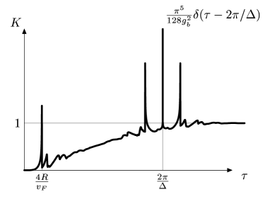
FIG. 3.: Form factor for the two point correlation function $K(\tau)=\int d\omega e^{i\omega\tau}R_{2}(\omega)$ for $g_{b}=5$. The $\delta$-function at $\tau=2\pi/\Delta$ is shown as a vertical spike. It arises because of the non-decaying oscillations (67). The $1/\sqrt{T_{2}-\tau}$ singularity at $T_{2}=4R/v_{F}$ is related to the “periodic orbit” which has period $T_{2}$ and traverses twice the diameter of the billiard. The same orbit gives rise to singularities at $\tau=2\pi/\Delta\pm T_{2}$

E Level number variance

In practice, the description of level statistics by the means of the level correlation function is not always convenient. Indeed, for low frequencies $\omega\ll v_{F}/R$ non-universal effects are manifested only as small corrections to RMT. For high frequencies, the entire behavior is non-universal, but in this range the level correlation function is proportional to $g_{b}^{-2}$ and small. Therefore, in order to study non-universal effects in level statistics, experimentally or by means of computer simulations, it is instructive to consider a quantity more sensitive to these effects.

A well-known way to emphasize the high-energy behavior of the level correlation function is to study the variance of the number of levels in an energy interval of width $E=s\Delta$,

$$\Sigma_{2}(s)=\int_{-s}^{s}\left(s-|\tilde{s}|\right)R_{2}(\tilde{s})d\tilde{s},$$ (68)

Direct calculation gives for $s\ll g_{b}$ ($E\ll v_{F}/R$)

$$\pi^{2}\Sigma_{2}(s)=1+\gamma+\ln(2\pi s)+\frac{As^{2}}{2g_{b}^{2}}$$ (69)

and for $s\gg g_{b}$ ($E\gg v_{F}/R$)

$$\pi^{2}\Sigma_{2}(s) = 1+\gamma+\ln\frac{16g_{b}}{\pi^{2}}$$ (71)

$$-\frac{\pi^{2}}{16}\left(\frac{2g_{b}}{\pi s}\right)^{1/2}\cos\left(\frac{4s}{g_{b}}-\frac{\pi}{4}\right).$$

Here $\gamma\approx 0.577$ is Euler’s constant, and $A$ is defined by Eq.(51). The first three terms at the r.h.s. of Eq.(69) represent the RMT contribution, which is logarithmic in energy [40]. It is remarkable that the actual level number variance is always smaller than that given by RMT.

FIG. 4.: Level number variance $\Sigma_{2}(E)$ as a function of energy; $s=E/\Delta$. Curve 1 shows the RMT result, while curves 2 and 3 correspond to asymptotic regimes of low (69) and high (71) frequencies. The saturation value $\Sigma_{2}^{(0)}$ is given by Eq. (72).

As seen from Fig. 4, the two asymptotes (69) and (71) perfectly match in the intermediate regime, $s\sim g_{b}$ ($E\sim v_{F}/R$). Taken together, they provide a complete description of $\Sigma_{2}(s)$. According to Eq.(71), the level number variance saturates at the value

$$\Sigma_{2}^{(0)}=\pi^{-2}(1+\gamma+\ln(16g_{b}/\pi^{2}))\gg 1.$$ (72)

This saturation again confirms the conclusion that we have already made from analyzing the low-energy behavior of the level correlation function — the system of levels of our billiard is quite rigid, more rigid than in RMT. We also remark that a saturation of $\Sigma_{2}(s)$, as well as its oscillations on the scale set by the shortest periodic orbit, is predicted by Berry for a generic chaotic billiard [5, 41]. This behavior is also in agreement with the results for $\Sigma_{2}(s)$ found numerically for a tight-binding model with moderately strong disorder on boundary sites [25, 26, 42].

At the same time, we note that the behavior of $\Sigma_{2}(s)$ is quite different from that in other reference systems. Indeed, for both diffusive systems [36] and systems with bulk disorder in ballistic regime [18, 19, 20] the level number variance is greater than RMT. The energy at which $\Sigma_{2}$ is expected to saturate depends on the type of disorder. For short-range impurities (white noise random potential) arbitrarily short periodic orbits exist, and thus no saturation up to $\omega\sim E_{F}$ is expected. For a diffusive system and smooth random potential the diffusive dynamics lead to a linear increase of the level number variance, $\Sigma_{2}(s)\sim s/g_{d}$, for $s\gg g_{d}\sim\nu v_{F}l_{tr}$, while the shortest orbits have lengths of the order of the transport mean free path $l_{tr}$, causing the saturation of $\Sigma_{2}(s)$ at a parametrically larger value $s\sim v_{F}/(l_{tr}\Delta)$. Similarly, in “rough billiards” (slightly distorted integrable billiards [15, 17]) the level number variance is higher than in RMT and does not saturate until a value $s\sim v_{F}/R\Delta$ parametrically exceeding the effective Thouless energy, since the system is diffusive in the angular momentum space.

IV Parametric level statistics

A Introduction

In this Section, we study the parametric statistics of energy levels of our system. Specifically, we assume that the billiard is placed in a magnetic field, which plays the role of an external parameter.

Already a considerable amount is known on the subject (see Ref. [43] for review). In this paper we are interested in the parametric level correlation function

$$R_{\Phi}(\omega,B)=-1$$ (73)

$$+ (V\Delta)^{2}\left\langle\nu(E+\omega/2,\bar{B}+B/2)\nu(E-\omega/2,\bar{B}-B/2)\right\rangle,$$ (74)

where the mean magnetic field $\bar{B}$ is introduced in order to break time-reversal symmetry. The correlation function (73) has been previously investigated in the diagrammatic expansion [44], the $\sigma$-model approach [45, 37], the random matrix theory (by means of Dyson’s brownian motion model) [46, 47], and by semi-classical methods [48, 49]. The most remarkable observation of these works is that when the perturbation is weak and the frequency $\omega$ is low, the parametric correlation function is universal, i.e it does not depend on the type of the perturbation, provided it is properly rescaled, nor on any details of the system.

Below we study non-universal behavior of the parametric level correlation function (73). We use the $\sigma$-model formulation of parametric statistics developed in Ref. [45] to derive an analog of Altshuler-Shklovskii formula for this function and evaluate it explicitly for our model.

B Eigenvalues of the Liouville operator in magnetic field

The correlation function (73) may be obtained from the supersymmetric $\sigma$-model with the effective action (1) provided the operator $\nabla$ is replaced by the “gauge-invariant” combination $\nabla-(ie/2c)\Lambda\mathchoice{{\hbox{\boldmath$\displaystyle A$}}}{{\hbox{\boldmath$\textstyle A$}}}{{\hbox{\boldmath$\scriptstyle A$}}}{{\hbox{\boldmath$\scriptscriptstyle A$}}}$, where $\textstyle A$ is the vector potential which corresponds to the field $B$: $B=\nabla\times\mathchoice{{\hbox{\boldmath$\displaystyle A$}}}{{\hbox{\boldmath$\textstyle A$}}}{{\hbox{\boldmath$\scriptstyle A$}}}{{\hbox{\boldmath$\scriptscriptstyle A$}}}$. Repeating the steps leading to Eq. (3) we find that in the effective action the Liouville operator $\hat{K}$ is replaced by its gauge-invariant form in the magnetic field,

$$\hat{K}_{\Phi}=v_{F}\mathchoice{{\hbox{\boldmath$\displaystyle n$}}}{{\hbox{\boldmath$\textstyle n$}}}{{\hbox{\boldmath$\scriptstyle n$}}}{{\hbox{\boldmath$\scriptscriptstyle n$}}}\left(\nabla-\frac{ie}{c}\mathchoice{{\hbox{\boldmath$\displaystyle A$}}}{{\hbox{\boldmath$\textstyle A$}}}{{\hbox{\boldmath$\scriptstyle A$}}}{{\hbox{\boldmath$\scriptscriptstyle A$}}}\right).$$ (75)

Prior to the investigation of statistical properties of the energy levels, we find the eigenvalues of the operator $\hat{K}_{\Phi}$. Choosing the symmetric gauge $\mathchoice{{\hbox{\boldmath$\displaystyle A$}}}{{\hbox{\boldmath$\textstyle A$}}}{{\hbox{\boldmath$\scriptstyle A$}}}{{\hbox{\boldmath$\scriptscriptstyle A$}}}=\mathchoice{{\hbox{\boldmath$\displaystyle B$}}}{{\hbox{\boldmath$\textstyle B$}}}{{\hbox{\boldmath$\scriptstyle B$}}}{{\hbox{\boldmath$\scriptscriptstyle B$}}}\times\mathchoice{{\hbox{\boldmath$\displaystyle r$}}}{{\hbox{\boldmath$\textstyle r$}}}{{\hbox{\boldmath$\scriptstyle r$}}}{{\hbox{\boldmath$\scriptscriptstyle r$}}}/2$ we obtain, instead of Eq. (14), the equation

$$J^{\phi}_{l}(\xi)\equiv-1$$ (76)

$$+ \frac{1}{2}\int_{0}^{\pi}d\theta\ \sin\theta\exp\left[2il\theta+2\xi\sin\theta+i\phi\sin 2\theta\right]=0,$$ (77)

which determines the dependence of the eigenvalue $\lambda_{l}=\xi v_{F}/R$ on the magnetic field. We have introduced the dimensionless parameter $\phi=\Phi/\Phi_{0}$, where $\Phi=\pi BR^{2}$ is the magnetic flux through the billiard, and $\Phi_{0}=2\pi\hbar c/e$ is the flux quantum.

Equation (76) defines a two-parameter set of eigenvalues $\xi_{kl}$. It stays invariant under the simultaneous transformations $l\to-l$, $\xi\to\xi^{*}$, $\phi\to-\phi$, which means that if $\lambda(B)$ is an eigenvalue of the operator $\hat{K}_{\Phi}$ then $\lambda^{*}(-B)$ is also an eigenvalue.

For sufficiently low frequencies and magnetic fields the parametric correlation function (73) is dominated by the zero mode $l=k=0$ (see below). To find the evolution of the corresponding eigenvalue $\xi_{00}$, we put $l=0$ and take a variation of Eq. (76) with respect to $\phi\ll 1$,

$$\int_{0}^{\pi}d\theta\ \sin\theta\left[2\xi_{00}\sin\theta+i\phi\sin 2\theta-\frac{\phi^{2}}{2}\sin^{2}2\theta\right]=0,$$

which gives $\xi_{00}=8\phi^{2}/(15\pi)$.

C Parametric level correlation function

The parametric correlation function $R_{\Phi}$ (73) is expressed in terms of the retarded $G^{R}$ and advanced $G^{A}$ Green’s functions in the following way,

$$R_{\Phi}(\omega,B) = \frac{1}{2}\left[T(\omega,B)+T(-\omega,-B)\right],$$ (78)

$$T(\omega,B) \equiv \frac{1}{2(\pi\nu)^{2}}\left\langle\mbox{\rm Tr}\ G^{R}(E+\omega/2,\bar{B}+B/2)\right.$$ (79)

$$\times \left.\mbox{\rm Tr}\ G^{A}(E-\omega/2,\bar{B}-B/2)\right\rangle_{c},$$ (80)

where $\langle AB\rangle_{c}\equiv\langle AB\rangle-\langle A\rangle\langle B\rangle$ denotes the irreducible part (cumulant).

For low frequencies and magnetic fields (the precise condition is specified below) the function $R_{\Phi}$ is non-perturbative and can be found using the random matrix theory. This regime was previously investigated in Ref. [45]. Here we focus instead on the case of higher frequencies and/or fields, when the smooth part of the parametric correlation function $R^{AS}_{\Phi}(\omega,B)$ is correctly described by perturbation theory. From Eq. (78) we obtain

$$R^{AS}_{\Phi}(\omega,B)$$ (81)

$$= \frac{\Delta^{2}}{4\pi^{2}}\mbox{\rm Re}\sum_{kl}\left\{\frac{1}{[-i\omega+\lambda_{kl}(B)]^{2}}+\frac{1}{[i\omega+\lambda_{kl}(-B)]^{2}}\right\}$$ (82)

$$= \frac{\Delta^{2}}{2\pi^{2}}\mbox{\rm Re}\sum_{kl}\frac{1}{[-i\omega+\lambda_{kl}(B)]^{2}}.$$ (83)

To identify relevant parameters, we consider $R^{AS}_{\Phi}$ at zero frequency. For low fields, the sum in Eq. (81) is dominated by the lowest eigenmode, which as we have seen is quadratic in field, $\lambda_{00}\sim v_{F}\phi^{2}/R$. The perturbation theory does not apply for $\lambda_{00}\lesssim\Delta$, which corresponds to the fields $\phi\lesssim g_{b}^{-1/2}$, where as before $g_{b}=v_{F}/(R\Delta)$. Generally, a non-perturbative calculation is needed when $\omega\lesssim\Delta$ and $\phi\lesssim g_{b}^{-1/2}$ (region 1 in Fig. 5). Everywhere outside this regime, the perturbative expression (81) applies.

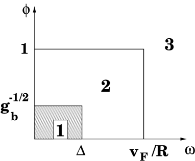
FIG. 5.: Different parameter regions (in the frequency – magnetic field plane) for the parametric level statistics: 1 – non-perturbative (RMT) region, 2 – zero-mode region, 3 – Altshuler-Shklovskii region

For higher fields, the zero mode still dominates until $\phi\sim 1$. At $\phi\sim 1$ other modes become important, and, in addition, the zero-mode eigenvalue can not be taken quadratic in field any more. Thus, the point $\phi\sim 1$ plays for parametric correlations the same role as $\omega\sim v_{F}/R$ for the usual (non-parametric) level correlation function. Generally, for $\phi\ll 1$ and $\omega\ll v_{F}/R$ we are in the regime when everything is determined by the zero-mode approximation. For higher fields $\phi\gg 1$ or frequencies $\omega\gg v_{F}/R$, the system crosses over to the Altshuler-Shklovskii regime (region 3 in Fig. 5), when all the modes are important.

To end our qualitative discussion, we determine the strength of the magnetic field needed to strongly affect the classical dynamics. The cyclotron radius of an electron trajectory in the magnetic field is $r_{c}=mv_{F}c/(eB)$. The magnetic field strongly affects the dynamics provided $r_{c}\lesssim R$, which gives $\phi\gtrsim g_{b}$. Our theory is thus valid for $\phi\ll g_{b}$, which still leaves a large window for the regime $\phi\gg 1$.

1 Perturbative zero-mode regime (Region 2 in Fig. 5)

Using the result for the zero-mode eigenvalue, we find from Eq. (81)

$$R^{AS}_{\Phi}(s,\phi)=\frac{225}{2}\frac{64g_{b}^{2}\phi^{4}-225\pi^{2}s^{2}}{(64g_{b}^{2}\phi^{4}+225\pi^{2}s^{2})^{2}},$$ (84)

where, as previously, $s=\omega/\Delta$. The result (84) applies when both $\phi\ll 1$ and $s\ll g_{b}$, but either $\phi\gg g_{b}^{-1/2}$ or $s\gg 1$. Without the magnetic field, $\phi=0$ and we reproduce $R^{AS}_{\Phi}(s,0)=-(2\pi^{2}s^{2})^{-1}$, which is a smooth version of the RMT result (46). For $s=0$, we obtain

$$R^{AS}_{\Phi}(0,\phi)=\frac{225}{128g_{b}^{2}\phi^{4}}.$$

2 Altshuler-Shklovskii regime (Region 3 in Fig. 5)

For $\phi\gg 1$ or $s\gg g_{b}$ we generalize Eq. (50) to the case of parametric statistics,

$$R^{AS}_{\Phi}(s,\phi)=-\frac{1}{2\pi^{2}g_{b}^{2}}\mbox{\rm Re}\sum_{l}\left.\frac{d^{2}}{dz^{2}}\right|_{z=is/g_{b}}\ln J_{l}^{\phi}(z),$$ (85)

and use the fact that $J_{l}^{\phi}\simeq-1$. Expanding $\ln J_{l}^{\phi}(z)$ in $J_{l}^{\phi}+1$ up to the second order, we obtain

$$R^{AS}_{\Phi}(s,\phi) = -\frac{1}{2\pi^{2}g_{b}^{2}}\mbox{\rm Re}\left.\sum_{l}\left\{-2\int_{0}^{\pi}d\theta\ \sin\theta\exp(2il\theta+2z\sin\theta+i\phi\sin 2\theta)\right.\right.$$ (86)

$$- \Biggl{.}\Biggl{.}\frac{1}{8}\frac{d^{2}}{dz^{2}}\int_{0}^{\pi}d\theta_{1}d\theta_{2}\sin\theta_{1}\sin\theta_{2}\exp\left[2il(\theta_{1}+\theta_{2})+2z(\sin\theta_{1}+\sin\theta_{2})+i\phi(\sin 2\theta_{1}+\sin 2\theta_{2})\right]\Biggr{\}}\Biggr{|}_{z=is/g_{b}}.$$ (87)

Now we employ the Poisson formula (62). The first integral in Eq. (86) vanishes identically, and in the second one we have $\theta_{1}+\theta_{2}=\pi$. Under this condition, the integral does not depend on the magnetic field. We thus have

$$R^{AS}_{\Phi}(s,\phi) = \frac{1}{\pi g_{b}^{2}}\mbox{\rm Re}\int_{0}^{\pi}d\theta\ \sin^{4}\theta\exp(4is\sin\theta/g_{b})$$ (88)

$$\approx \left\{\matrix{(8g_{b}^{2})^{-1}(3-20s^{2}/g_{b}^{2}),&s\ll g_{b}\cr(2\pi sg_{b}^{3})^{-1/2}\cos(4s/g_{b}-\pi/4),&s\gg g_{b}}\right..$$ (89)

The asymptotes in the regime $s\gg g_{b}$ are identical to Eq. (63).

The result that the parametric level correlation function does not decay with magnetic field is very different from the diffusive case [37] and is actually quite surprising. It means that the density of states at the same energy retains the memory even at very large fields, after the levels underwent many avoided crossings. The field dependence of the correlator appears if we keep higher orders of the expansion of the logarithm in Eq. (85), but it is only manifested as small corrections to the result (88).

D Parametric level number variance

The high-frequency behavior of the non-parametric level correlation function $R_{2}(s)$ is best seen in the level number variance $\Sigma_{2}(s)$, see Section III. Similarly, it is instructive to introduce the parametric level number variance (PLNV)[48],

$$U(E,B)=\left\langle\left[N(E,\bar{B})-N(E,\bar{B}+B)\right]^{2}\right\rangle,$$ (90)

where $N(E,B)$ is the full number of levels in the energy strip $E$ in the magnetic field $B$. In zero field PLNV vanishes (in low fields it is generally linear in field, see Ref. [45]). If the values of $N(E,B)$ and $N(E,\bar{B}+B)$ are uncorrelated in high fields (which is not the case in our situation, since the level correlation function does not decay in high fields), PLNV saturates, $U(E,B\to\infty)\to 2\Sigma_{2}(E)$.

PLNV can be easily expressed through the level correlation function (analogously to Eq. (68)),

$$U(s,\phi)=2\int_{-s}^{s}(s-|\tilde{s}|)\left[R_{2}(\tilde{s})-R_{\Phi}(\tilde{s},\phi)\right]d\tilde{s},$$ (91)

where $s=E/\Delta$. Below we concentrate on the perturbative regime $\phi\gg g_{b}^{-1/2}$, when

$$\int_{-s}^{s}(s-|\tilde{s}|)R_{\Phi}(\tilde{s},\phi)d\tilde{s}$$ (92)

$$\approx \frac{1}{\pi^{2}}\mbox{\rm Re}\sum_{l}\left[\ln J_{l}^{\phi}(is/g_{b})-\ln J_{l}^{\phi}(0)\right].$$ (93)

A direct calculation gives for $g_{b}^{-1/2}\ll\phi\ll 1$

$$U(s,\phi) = \frac{2}{\pi^{2}}(\ln 2\pi s+1+\gamma)-\frac{225}{128}\frac{s^{2}}{g_{b}^{2}\phi^{4}},$$ (95)

$$\ \ \ \ \ \ \ \ \ \ \ 1\ll s\ll g_{b}\phi^{2},$$

$$U(s,\phi) = \frac{2}{\pi^{2}}\left[\ln\frac{8g_{b}\phi^{2}}{15}+1+\gamma\right],\ \ \ g_{b}\phi^{2}\ll s\ll g_{b},$$ (96)

$$U(s,\phi) = \frac{2}{\pi^{2}}\left[\ln\frac{32g_{b}\phi^{2}}{15}+1+\gamma\right]-A^{\prime},\ \ \ s\gg g_{b},$$ (97)

where $\gamma$ is again Euler’s constant, and

$$A^{\prime}=-\frac{2}{\pi^{2}}\sum_{l=1}^{\infty}\ln\left(1-\frac{1}{4l^{2}-1}\right)\approx 0.115.$$

In higher fields $\phi\gg 1$ we have

$$U(s,\phi) = \frac{2}{\pi^{2}}(\ln 2\pi s+1+\gamma)+\frac{s^{2}}{g_{b}^{2}}\left(\frac{A}{\pi^{2}}-\frac{3}{2}\right),$$ (99)

$$\ \ \ \ \ \ \ \ \ \ \ 1\ll s\ll g_{b},$$

$$U(s,\phi) = \frac{2}{\pi^{2}}\left[\ln\frac{16g_{b}}{\pi^{2}}+1+\gamma\right]-\frac{1}{8},\ \ \ s\gg g_{b},$$ (100)

where the constant $A$ is given by Eq. (51). A comparison of Eq. (99) with Eqs. (69) and (71) shows that in the limit $\phi\to\infty$ PLNV differs from $2\Sigma_{2}(s)$. This difference originates from the fact that the correlation function $R_{\Phi}$ does not vanish at large $\phi$ (see Eq. (88)).

V Correlations of eigenfunctions

According to Berry’s conjecture [50], a wave function in a 2D chaotic system shows Gaussian fluctuations with the correlation function $V\langle\psi^{*}({\mathchoice{{\hbox{\boldmath$\displaystyle r$}}}{{\hbox{\boldmath$\textstyle r$}}}{{\hbox{\boldmath$\scriptstyle r$}}}{{\hbox{\boldmath$\scriptscriptstyle r$}}}})\psi({\mathchoice{{\hbox{\boldmath$\displaystyle r$}}}{{\hbox{\boldmath$\textstyle r$}}}{{\hbox{\boldmath$\scriptstyle r$}}}{{\hbox{\boldmath$\scriptscriptstyle r$}}}^{\prime}})\rangle=J_{0}(p_{F}r)$ (see Ref.[51] for a recent generalization of this conjecture). The supersymmetry method allows one to derive this result (which is equivalent to the zero-mode approximation for the $\sigma$-model) and to calculate system-specific corrections [52, 53, 54, 55, 8] .

Let us consider the two-point correlation function

$$C(\mathchoice{{\hbox{\boldmath$\displaystyle r$}}}{{\hbox{\boldmath$\textstyle r$}}}{{\hbox{\boldmath$\scriptstyle r$}}}{{\hbox{\boldmath$\scriptscriptstyle r$}}}_{1},\mathchoice{{\hbox{\boldmath$\displaystyle r$}}}{{\hbox{\boldmath$\textstyle r$}}}{{\hbox{\boldmath$\scriptstyle r$}}}{{\hbox{\boldmath$\scriptscriptstyle r$}}}_{2})=\Delta\left\langle\sum_{\alpha}|\psi_{\alpha}^{2}(\mathchoice{{\hbox{\boldmath$\displaystyle r$}}}{{\hbox{\boldmath$\textstyle r$}}}{{\hbox{\boldmath$\scriptstyle r$}}}{{\hbox{\boldmath$\scriptscriptstyle r$}}}_{1})\psi_{\alpha}^{2}(\mathchoice{{\hbox{\boldmath$\displaystyle r$}}}{{\hbox{\boldmath$\textstyle r$}}}{{\hbox{\boldmath$\scriptstyle r$}}}{{\hbox{\boldmath$\scriptscriptstyle r$}}}_{2})|\delta(\epsilon-\epsilon_{\alpha})\right\rangle\ .$$ (101)

In the standard diffusive $\sigma$-model [8], the correlation function (101) can be written in the form of the integral over the $\sigma$-model field Q(r),

$$C(\mathchoice{{\hbox{\boldmath$\displaystyle r$}}}{{\hbox{\boldmath$\textstyle r$}}}{{\hbox{\boldmath$\scriptstyle r$}}}{{\hbox{\boldmath$\scriptscriptstyle r$}}}_{1},\mathchoice{{\hbox{\boldmath$\displaystyle r$}}}{{\hbox{\boldmath$\textstyle r$}}}{{\hbox{\boldmath$\scriptstyle r$}}}{{\hbox{\boldmath$\scriptscriptstyle r$}}}_{2}) = \lim_{\eta\to 0}{\eta\Delta\over\pi}\langle G_{11}(\mathchoice{{\hbox{\boldmath$\displaystyle r$}}}{{\hbox{\boldmath$\textstyle r$}}}{{\hbox{\boldmath$\scriptstyle r$}}}{{\hbox{\boldmath$\scriptscriptstyle r$}}}_{1},\mathchoice{{\hbox{\boldmath$\displaystyle r$}}}{{\hbox{\boldmath$\textstyle r$}}}{{\hbox{\boldmath$\scriptstyle r$}}}{{\hbox{\boldmath$\scriptscriptstyle r$}}}_{1})G_{22}(\mathchoice{{\hbox{\boldmath$\displaystyle r$}}}{{\hbox{\boldmath$\textstyle r$}}}{{\hbox{\boldmath$\scriptstyle r$}}}{{\hbox{\boldmath$\scriptscriptstyle r$}}}_{2},\mathchoice{{\hbox{\boldmath$\displaystyle r$}}}{{\hbox{\boldmath$\textstyle r$}}}{{\hbox{\boldmath$\scriptstyle r$}}}{{\hbox{\boldmath$\scriptscriptstyle r$}}}_{2})$$ (102)

$$+ G_{12}(\mathchoice{{\hbox{\boldmath$\displaystyle r$}}}{{\hbox{\boldmath$\textstyle r$}}}{{\hbox{\boldmath$\scriptstyle r$}}}{{\hbox{\boldmath$\scriptscriptstyle r$}}}_{1},\mathchoice{{\hbox{\boldmath$\displaystyle r$}}}{{\hbox{\boldmath$\textstyle r$}}}{{\hbox{\boldmath$\scriptstyle r$}}}{{\hbox{\boldmath$\scriptscriptstyle r$}}}_{2})G_{21}(\mathchoice{{\hbox{\boldmath$\displaystyle r$}}}{{\hbox{\boldmath$\textstyle r$}}}{{\hbox{\boldmath$\scriptstyle r$}}}{{\hbox{\boldmath$\scriptscriptstyle r$}}}_{2},\mathchoice{{\hbox{\boldmath$\displaystyle r$}}}{{\hbox{\boldmath$\textstyle r$}}}{{\hbox{\boldmath$\scriptstyle r$}}}{{\hbox{\boldmath$\scriptscriptstyle r$}}}_{1})\rangle_{{\cal S}[Q]}\ ,$$ (103)

where $\eta=-i\omega/2>0$ is the level broadening, $G$ is the Green’s function in the field $Q$, and the subscripts $1,2$ refer to the advanced-retarded decomposition, the boson-boson components being always implied (we drop the corresponding indices). Eq. (103) yields the following result [54],

$$V^{2}C(\mathchoice{{\hbox{\boldmath$\displaystyle r$}}}{{\hbox{\boldmath$\textstyle r$}}}{{\hbox{\boldmath$\scriptstyle r$}}}{{\hbox{\boldmath$\scriptscriptstyle r$}}}_{1},\mathchoice{{\hbox{\boldmath$\displaystyle r$}}}{{\hbox{\boldmath$\textstyle r$}}}{{\hbox{\boldmath$\scriptstyle r$}}}{{\hbox{\boldmath$\scriptscriptstyle r$}}}_{2})\simeq 1+\Pi_{D}(\mathchoice{{\hbox{\boldmath$\displaystyle r$}}}{{\hbox{\boldmath$\textstyle r$}}}{{\hbox{\boldmath$\scriptstyle r$}}}{{\hbox{\boldmath$\scriptscriptstyle r$}}}_{1},\mathchoice{{\hbox{\boldmath$\displaystyle r$}}}{{\hbox{\boldmath$\textstyle r$}}}{{\hbox{\boldmath$\scriptstyle r$}}}{{\hbox{\boldmath$\scriptscriptstyle r$}}}_{2})+k_{q}(\mathchoice{{\hbox{\boldmath$\displaystyle r$}}}{{\hbox{\boldmath$\textstyle r$}}}{{\hbox{\boldmath$\scriptstyle r$}}}{{\hbox{\boldmath$\scriptscriptstyle r$}}}_{1}-\mathchoice{{\hbox{\boldmath$\displaystyle r$}}}{{\hbox{\boldmath$\textstyle r$}}}{{\hbox{\boldmath$\scriptstyle r$}}}{{\hbox{\boldmath$\scriptscriptstyle r$}}}_{2})$$ (104)

$$+\Pi_{D}\left({\mathchoice{{\hbox{\boldmath$\displaystyle r$}}}{{\hbox{\boldmath$\textstyle r$}}}{{\hbox{\boldmath$\scriptstyle r$}}}{{\hbox{\boldmath$\scriptscriptstyle r$}}}_{1}+\mathchoice{{\hbox{\boldmath$\displaystyle r$}}}{{\hbox{\boldmath$\textstyle r$}}}{{\hbox{\boldmath$\scriptstyle r$}}}{{\hbox{\boldmath$\scriptscriptstyle r$}}}_{2}\over 2},{\mathchoice{{\hbox{\boldmath$\displaystyle r$}}}{{\hbox{\boldmath$\textstyle r$}}}{{\hbox{\boldmath$\scriptstyle r$}}}{{\hbox{\boldmath$\scriptscriptstyle r$}}}_{1}+\mathchoice{{\hbox{\boldmath$\displaystyle r$}}}{{\hbox{\boldmath$\textstyle r$}}}{{\hbox{\boldmath$\scriptstyle r$}}}{{\hbox{\boldmath$\scriptscriptstyle r$}}}_{2}\over 2}\right)k_{q}(\mathchoice{{\hbox{\boldmath$\displaystyle r$}}}{{\hbox{\boldmath$\textstyle r$}}}{{\hbox{\boldmath$\scriptstyle r$}}}{{\hbox{\boldmath$\scriptscriptstyle r$}}}_{1}-\mathchoice{{\hbox{\boldmath$\displaystyle r$}}}{{\hbox{\boldmath$\textstyle r$}}}{{\hbox{\boldmath$\scriptstyle r$}}}{{\hbox{\boldmath$\scriptscriptstyle r$}}}_{2}),$$ (105)

where $\Pi_{D}$ is the diffusion propagator, $k_{q}(r)=J_{0}^{2}(p_{F}r)e^{-r/l}$, and $l$ is the mean free path. In the framework of the ballistic $\sigma$-model the diffusive propagator $\Pi_{D}(\mathchoice{{\hbox{\boldmath$\displaystyle r$}}}{{\hbox{\boldmath$\textstyle r$}}}{{\hbox{\boldmath$\scriptstyle r$}}}{{\hbox{\boldmath$\scriptscriptstyle r$}}}_{1},\mathchoice{{\hbox{\boldmath$\displaystyle r$}}}{{\hbox{\boldmath$\textstyle r$}}}{{\hbox{\boldmath$\scriptstyle r$}}}{{\hbox{\boldmath$\scriptscriptstyle r$}}}_{2})$ is replaced by its ballistic counterpart $\Pi_{B}(\mathchoice{{\hbox{\boldmath$\displaystyle r$}}}{{\hbox{\boldmath$\textstyle r$}}}{{\hbox{\boldmath$\scriptstyle r$}}}{{\hbox{\boldmath$\scriptscriptstyle r$}}}_{1},\mathchoice{{\hbox{\boldmath$\displaystyle r$}}}{{\hbox{\boldmath$\textstyle r$}}}{{\hbox{\boldmath$\scriptstyle r$}}}{{\hbox{\boldmath$\scriptscriptstyle r$}}}_{2})$ given in our model by Eq. (32). At this point we seem to encounter a problem. Indeed, at short distances $r=|\mathchoice{{\hbox{\boldmath$\displaystyle r$}}}{{\hbox{\boldmath$\textstyle r$}}}{{\hbox{\boldmath$\scriptstyle r$}}}{{\hbox{\boldmath$\scriptscriptstyle r$}}}_{1}-\mathchoice{{\hbox{\boldmath$\displaystyle r$}}}{{\hbox{\boldmath$\textstyle r$}}}{{\hbox{\boldmath$\scriptstyle r$}}}{{\hbox{\boldmath$\scriptscriptstyle r$}}}_{2}|$ the classical propagator $\Pi_{B}(\mathchoice{{\hbox{\boldmath$\displaystyle r$}}}{{\hbox{\boldmath$\textstyle r$}}}{{\hbox{\boldmath$\scriptstyle r$}}}{{\hbox{\boldmath$\scriptscriptstyle r$}}}_{1},\mathchoice{{\hbox{\boldmath$\displaystyle r$}}}{{\hbox{\boldmath$\textstyle r$}}}{{\hbox{\boldmath$\scriptstyle r$}}}{{\hbox{\boldmath$\scriptscriptstyle r$}}}_{2})$ is dominated by the contribution of the direct path,

$$\Pi_{B}(\mathchoice{{\hbox{\boldmath$\displaystyle r$}}}{{\hbox{\boldmath$\textstyle r$}}}{{\hbox{\boldmath$\scriptstyle r$}}}{{\hbox{\boldmath$\scriptscriptstyle r$}}}_{1},\mathchoice{{\hbox{\boldmath$\displaystyle r$}}}{{\hbox{\boldmath$\textstyle r$}}}{{\hbox{\boldmath$\scriptstyle r$}}}{{\hbox{\boldmath$\scriptscriptstyle r$}}}_{2})\simeq f_{0}(\mathchoice{{\hbox{\boldmath$\displaystyle r$}}}{{\hbox{\boldmath$\textstyle r$}}}{{\hbox{\boldmath$\scriptstyle r$}}}{{\hbox{\boldmath$\scriptscriptstyle r$}}}_{1},\mathchoice{{\hbox{\boldmath$\displaystyle r$}}}{{\hbox{\boldmath$\textstyle r$}}}{{\hbox{\boldmath$\scriptstyle r$}}}{{\hbox{\boldmath$\scriptscriptstyle r$}}}_{2})={1\over\pi p_{F}|\mathchoice{{\hbox{\boldmath$\displaystyle r$}}}{{\hbox{\boldmath$\textstyle r$}}}{{\hbox{\boldmath$\scriptstyle r$}}}{{\hbox{\boldmath$\scriptscriptstyle r$}}}_{1}-\mathchoice{{\hbox{\boldmath$\displaystyle r$}}}{{\hbox{\boldmath$\textstyle r$}}}{{\hbox{\boldmath$\scriptstyle r$}}}{{\hbox{\boldmath$\scriptscriptstyle r$}}}_{2}|}\ .$$ (106)

This contribution, which becomes of order unity at $r\sim\lambda_{F}$, would imply strong deviations from the universal Gaussian statistics. However, it is not difficult to realize that this contribution is nothing else but a classical “copy” of the term $k_{q}(\mathchoice{{\hbox{\boldmath$\displaystyle r$}}}{{\hbox{\boldmath$\textstyle r$}}}{{\hbox{\boldmath$\scriptstyle r$}}}{{\hbox{\boldmath$\scriptscriptstyle r$}}}_{1}-\mathchoice{{\hbox{\boldmath$\displaystyle r$}}}{{\hbox{\boldmath$\textstyle r$}}}{{\hbox{\boldmath$\scriptstyle r$}}}{{\hbox{\boldmath$\scriptscriptstyle r$}}}_{2})$. Therefore, we encounter a problem of the double counting: one and the same contribution is taken into account twice, classically and quantum-mechanically. In the case of the diffusive $\sigma$-model this problem does not appear because of the scale separation: the classical propagator $\Pi_{D}$ is restricted to low momenta $q<l^{-1}$, while the short-scale ($r<l$) physics corresponding to high momenta ($q>l^{-1}$) is treated quantum-mechanically.

The situation is different in ballistic case. The semi-classical description extends now to all momenta $q\lesssim p_{F}$. Therefore, there is no separation in momentum space between the slow modes (treated within the semi-classical approximation) and the fast ones (treated exactly, i.e. quantum-mechanically), and a careful treatment is required in order to avoid the double counting. For this purpose, we find it instructive to consider a problem with an additional smooth random potential $U({\mathchoice{{\hbox{\boldmath$\displaystyle r$}}}{{\hbox{\boldmath$\textstyle r$}}}{{\hbox{\boldmath$\scriptstyle r$}}}{{\hbox{\boldmath$\scriptscriptstyle r$}}}})$ in the bulk, characterized by a correlation function $V({\mathchoice{{\hbox{\boldmath$\displaystyle r$}}}{{\hbox{\boldmath$\textstyle r$}}}{{\hbox{\boldmath$\scriptstyle r$}}}{{\hbox{\boldmath$\scriptscriptstyle r$}}}}-{\mathchoice{{\hbox{\boldmath$\displaystyle r$}}}{{\hbox{\boldmath$\textstyle r$}}}{{\hbox{\boldmath$\scriptstyle r$}}}{{\hbox{\boldmath$\scriptscriptstyle r$}}}^{\prime}})=\langle U({\mathchoice{{\hbox{\boldmath$\displaystyle r$}}}{{\hbox{\boldmath$\textstyle r$}}}{{\hbox{\boldmath$\scriptstyle r$}}}{{\hbox{\boldmath$\scriptscriptstyle r$}}}})U({\mathchoice{{\hbox{\boldmath$\displaystyle r$}}}{{\hbox{\boldmath$\textstyle r$}}}{{\hbox{\boldmath$\scriptstyle r$}}}{{\hbox{\boldmath$\scriptscriptstyle r$}}}^{\prime}})\rangle$ with a correlation length $d\gg\lambda_{F}$ and inducing a small-angle scattering. Specifically, we will assume that the corresponding transport scattering rate $\tau_{tr}^{-1}$ is negligible, i.e. the transport mean free path $l_{tr}=v_{F}\tau_{tr}$ is large, $l_{tr}\gg R$, so that the bulk scattering has essentially no effect on the classical dynamics. On the other hand, the single-particle mean free path $l=v_{F}\tau$ (corresponding to the total relaxation rate $\tau^{-1}$) will be assumed to satisfy $\lambda_{F}\ll d\ll l\ll R$ and will play a role similar to that of $l_{tr}$ for the diffusive $\sigma$-model, separating the regions of classical and quantum treatment. The condition $d\ll l$ ensures that the scattering on this random potential is of quantum-mechanical (rather than classical) nature and is correctly treated within the Born approximation.

We first ignore the boundary scattering and will return to it in the end of the calculation. Averaging over the realizations of the smooth random potential $U({\mathchoice{{\hbox{\boldmath$\displaystyle r$}}}{{\hbox{\boldmath$\textstyle r$}}}{{\hbox{\boldmath$\scriptstyle r$}}}{{\hbox{\boldmath$\scriptscriptstyle r$}}}})$, one can derive the $\sigma$-model following Ref. [56]. (This derivation is outlined in Appendix).

To calculate deviations of the eigenfunction statistics from universality, we write [8, 35, 53, 54] (See Eq. (A6))

$$T({\mathchoice{{\hbox{\boldmath$\displaystyle r$}}}{{\hbox{\boldmath$\textstyle r$}}}{{\hbox{\boldmath$\scriptstyle r$}}}{{\hbox{\boldmath$\scriptscriptstyle r$}}}},{\mathchoice{{\hbox{\boldmath$\displaystyle n$}}}{{\hbox{\boldmath$\textstyle n$}}}{{\hbox{\boldmath$\scriptstyle n$}}}{{\hbox{\boldmath$\scriptscriptstyle n$}}}})=T_{0}(1-W({\mathchoice{{\hbox{\boldmath$\displaystyle r$}}}{{\hbox{\boldmath$\textstyle r$}}}{{\hbox{\boldmath$\scriptstyle r$}}}{{\hbox{\boldmath$\scriptscriptstyle r$}}}},{\mathchoice{{\hbox{\boldmath$\displaystyle n$}}}{{\hbox{\boldmath$\textstyle n$}}}{{\hbox{\boldmath$\scriptstyle n$}}}{{\hbox{\boldmath$\scriptscriptstyle n$}}}})/2)\ ,$$ (107)

and then integrate out perturbatively non-zero modes described by $W({\mathchoice{{\hbox{\boldmath$\displaystyle r$}}}{{\hbox{\boldmath$\textstyle r$}}}{{\hbox{\boldmath$\scriptstyle r$}}}{{\hbox{\boldmath$\scriptscriptstyle r$}}}},{\mathchoice{{\hbox{\boldmath$\displaystyle n$}}}{{\hbox{\boldmath$\textstyle n$}}}{{\hbox{\boldmath$\scriptstyle n$}}}{{\hbox{\boldmath$\scriptscriptstyle n$}}}})$. The part of action (A7) which is quadratic in $W$ has the following form in the momentum space,

$$F_{0} = {1\over 2}{\rm Str}\int d{\mathchoice{{\hbox{\boldmath$\displaystyle n$}}}{{\hbox{\boldmath$\textstyle n$}}}{{\hbox{\boldmath$\scriptstyle n$}}}{{\hbox{\boldmath$\scriptscriptstyle n$}}}}_{1}d{\mathchoice{{\hbox{\boldmath$\displaystyle n$}}}{{\hbox{\boldmath$\textstyle n$}}}{{\hbox{\boldmath$\scriptstyle n$}}}{{\hbox{\boldmath$\scriptscriptstyle n$}}}}_{2}(d{\mathchoice{{\hbox{\boldmath$\displaystyle q$}}}{{\hbox{\boldmath$\textstyle q$}}}{{\hbox{\boldmath$\scriptstyle q$}}}{{\hbox{\boldmath$\scriptscriptstyle q$}}}})W_{21}(-{\mathchoice{{\hbox{\boldmath$\displaystyle q$}}}{{\hbox{\boldmath$\textstyle q$}}}{{\hbox{\boldmath$\scriptstyle q$}}}{{\hbox{\boldmath$\scriptscriptstyle q$}}}},{\mathchoice{{\hbox{\boldmath$\displaystyle n$}}}{{\hbox{\boldmath$\textstyle n$}}}{{\hbox{\boldmath$\scriptstyle n$}}}{{\hbox{\boldmath$\scriptscriptstyle n$}}}}_{1})W_{12}({\mathchoice{{\hbox{\boldmath$\displaystyle q$}}}{{\hbox{\boldmath$\textstyle q$}}}{{\hbox{\boldmath$\scriptstyle q$}}}{{\hbox{\boldmath$\scriptscriptstyle q$}}}},{\mathchoice{{\hbox{\boldmath$\displaystyle n$}}}{{\hbox{\boldmath$\textstyle n$}}}{{\hbox{\boldmath$\scriptstyle n$}}}{{\hbox{\boldmath$\scriptscriptstyle n$}}}}_{2})$$ (108)

$$\times \left(-{1\over 2}\int(d{\mathchoice{{\hbox{\boldmath$\displaystyle p$}}}{{\hbox{\boldmath$\textstyle p$}}}{{\hbox{\boldmath$\scriptstyle p$}}}{{\hbox{\boldmath$\scriptscriptstyle p$}}}})w({\mathchoice{{\hbox{\boldmath$\displaystyle n$}}}{{\hbox{\boldmath$\textstyle n$}}}{{\hbox{\boldmath$\scriptstyle n$}}}{{\hbox{\boldmath$\scriptscriptstyle n$}}}}_{1},{\mathchoice{{\hbox{\boldmath$\displaystyle n$}}}{{\hbox{\boldmath$\textstyle n$}}}{{\hbox{\boldmath$\scriptstyle n$}}}{{\hbox{\boldmath$\scriptscriptstyle n$}}}})w({\mathchoice{{\hbox{\boldmath$\displaystyle n$}}}{{\hbox{\boldmath$\textstyle n$}}}{{\hbox{\boldmath$\scriptstyle n$}}}{{\hbox{\boldmath$\scriptscriptstyle n$}}}},{\mathchoice{{\hbox{\boldmath$\displaystyle n$}}}{{\hbox{\boldmath$\textstyle n$}}}{{\hbox{\boldmath$\scriptstyle n$}}}{{\hbox{\boldmath$\scriptscriptstyle n$}}}}_{2})G_{R}({\mathchoice{{\hbox{\boldmath$\displaystyle p$}}}{{\hbox{\boldmath$\textstyle p$}}}{{\hbox{\boldmath$\scriptstyle p$}}}{{\hbox{\boldmath$\scriptscriptstyle p$}}}}_{+})G_{A}({\mathchoice{{\hbox{\boldmath$\displaystyle p$}}}{{\hbox{\boldmath$\textstyle p$}}}{{\hbox{\boldmath$\scriptstyle p$}}}{{\hbox{\boldmath$\scriptscriptstyle p$}}}}_{-})+\pi\nu w({\mathchoice{{\hbox{\boldmath$\displaystyle n$}}}{{\hbox{\boldmath$\textstyle n$}}}{{\hbox{\boldmath$\scriptstyle n$}}}{{\hbox{\boldmath$\scriptscriptstyle n$}}}}_{1},{\mathchoice{{\hbox{\boldmath$\displaystyle n$}}}{{\hbox{\boldmath$\textstyle n$}}}{{\hbox{\boldmath$\scriptstyle n$}}}{{\hbox{\boldmath$\scriptscriptstyle n$}}}}_{2})\right)$$ (109)

$$\equiv {1\over 2}{\rm Str}\int d{\mathchoice{{\hbox{\boldmath$\displaystyle n$}}}{{\hbox{\boldmath$\textstyle n$}}}{{\hbox{\boldmath$\scriptstyle n$}}}{{\hbox{\boldmath$\scriptscriptstyle n$}}}}_{1}d{\mathchoice{{\hbox{\boldmath$\displaystyle n$}}}{{\hbox{\boldmath$\textstyle n$}}}{{\hbox{\boldmath$\scriptstyle n$}}}{{\hbox{\boldmath$\scriptscriptstyle n$}}}}_{2}(d{\mathchoice{{\hbox{\boldmath$\displaystyle q$}}}{{\hbox{\boldmath$\textstyle q$}}}{{\hbox{\boldmath$\scriptstyle q$}}}{{\hbox{\boldmath$\scriptscriptstyle q$}}}})W_{21}(-{\mathchoice{{\hbox{\boldmath$\displaystyle q$}}}{{\hbox{\boldmath$\textstyle q$}}}{{\hbox{\boldmath$\scriptstyle q$}}}{{\hbox{\boldmath$\scriptscriptstyle q$}}}},{\mathchoice{{\hbox{\boldmath$\displaystyle n$}}}{{\hbox{\boldmath$\textstyle n$}}}{{\hbox{\boldmath$\scriptstyle n$}}}{{\hbox{\boldmath$\scriptscriptstyle n$}}}}_{1})W_{12}({\mathchoice{{\hbox{\boldmath$\displaystyle q$}}}{{\hbox{\boldmath$\textstyle q$}}}{{\hbox{\boldmath$\scriptstyle q$}}}{{\hbox{\boldmath$\scriptscriptstyle q$}}}},{\mathchoice{{\hbox{\boldmath$\displaystyle n$}}}{{\hbox{\boldmath$\textstyle n$}}}{{\hbox{\boldmath$\scriptstyle n$}}}{{\hbox{\boldmath$\scriptscriptstyle n$}}}}_{2})[-A({\mathchoice{{\hbox{\boldmath$\displaystyle q$}}}{{\hbox{\boldmath$\textstyle q$}}}{{\hbox{\boldmath$\scriptstyle q$}}}{{\hbox{\boldmath$\scriptscriptstyle q$}}}};{\mathchoice{{\hbox{\boldmath$\displaystyle n$}}}{{\hbox{\boldmath$\textstyle n$}}}{{\hbox{\boldmath$\scriptstyle n$}}}{{\hbox{\boldmath$\scriptscriptstyle n$}}}}_{1},{\mathchoice{{\hbox{\boldmath$\displaystyle n$}}}{{\hbox{\boldmath$\textstyle n$}}}{{\hbox{\boldmath$\scriptstyle n$}}}{{\hbox{\boldmath$\scriptscriptstyle n$}}}}_{2})+B({\mathchoice{{\hbox{\boldmath$\displaystyle n$}}}{{\hbox{\boldmath$\textstyle n$}}}{{\hbox{\boldmath$\scriptstyle n$}}}{{\hbox{\boldmath$\scriptscriptstyle n$}}}}_{1},{\mathchoice{{\hbox{\boldmath$\displaystyle n$}}}{{\hbox{\boldmath$\textstyle n$}}}{{\hbox{\boldmath$\scriptstyle n$}}}{{\hbox{\boldmath$\scriptscriptstyle n$}}}}_{2})]\ ,$$ (110)

where ${\mathchoice{{\hbox{\boldmath$\displaystyle p$}}}{{\hbox{\boldmath$\textstyle p$}}}{{\hbox{\boldmath$\scriptstyle p$}}}{{\hbox{\boldmath$\scriptscriptstyle p$}}}}_{\pm}={\mathchoice{{\hbox{\boldmath$\displaystyle p$}}}{{\hbox{\boldmath$\textstyle p$}}}{{\hbox{\boldmath$\scriptstyle p$}}}{{\hbox{\boldmath$\scriptscriptstyle p$}}}}\pm{\mathchoice{{\hbox{\boldmath$\displaystyle q$}}}{{\hbox{\boldmath$\textstyle q$}}}{{\hbox{\boldmath$\scriptstyle q$}}}{{\hbox{\boldmath$\scriptscriptstyle q$}}}}/2$. In the last line of (108) we introduced the definitions $A$ and $B$ for the two terms of the quadratic form. Eq. (108) induces the contraction rules for integrals over non-zero modes $W$ (cf. Ref. [57]),

$$\Bigl{\langle}\rm{Str}[W(-{\mathchoice{{\hbox{\boldmath$\displaystyle q$}}}{{\hbox{\boldmath$\textstyle q$}}}{{\hbox{\boldmath$\scriptstyle q$}}}{{\hbox{\boldmath$\scriptscriptstyle q$}}}},{\mathchoice{{\hbox{\boldmath$\displaystyle n$}}}{{\hbox{\boldmath$\textstyle n$}}}{{\hbox{\boldmath$\scriptstyle n$}}}{{\hbox{\boldmath$\scriptscriptstyle n$}}}}_{1})P]{\rm Str}[W({\mathchoice{{\hbox{\boldmath$\displaystyle q$}}}{{\hbox{\boldmath$\textstyle q$}}}{{\hbox{\boldmath$\scriptstyle q$}}}{{\hbox{\boldmath$\scriptscriptstyle q$}}}},{\mathchoice{{\hbox{\boldmath$\displaystyle n$}}}{{\hbox{\boldmath$\textstyle n$}}}{{\hbox{\boldmath$\scriptstyle n$}}}{{\hbox{\boldmath$\scriptscriptstyle n$}}}}_{2})R]\Bigr{\rangle}$$ (111)

$$=2{\cal D}({\mathchoice{{\hbox{\boldmath$\displaystyle q$}}}{{\hbox{\boldmath$\textstyle q$}}}{{\hbox{\boldmath$\scriptstyle q$}}}{{\hbox{\boldmath$\scriptscriptstyle q$}}}};{\mathchoice{{\hbox{\boldmath$\displaystyle n$}}}{{\hbox{\boldmath$\textstyle n$}}}{{\hbox{\boldmath$\scriptstyle n$}}}{{\hbox{\boldmath$\scriptscriptstyle n$}}}}_{2},{\mathchoice{{\hbox{\boldmath$\displaystyle n$}}}{{\hbox{\boldmath$\textstyle n$}}}{{\hbox{\boldmath$\scriptstyle n$}}}{{\hbox{\boldmath$\scriptscriptstyle n$}}}}_{1})\rm{Str}P{1-\Lambda\over 2}R{1+\Lambda\over 2}$$ (112)

$$+2{\cal D}(-{\mathchoice{{\hbox{\boldmath$\displaystyle q$}}}{{\hbox{\boldmath$\textstyle q$}}}{{\hbox{\boldmath$\scriptstyle q$}}}{{\hbox{\boldmath$\scriptscriptstyle q$}}}};{\mathchoice{{\hbox{\boldmath$\displaystyle n$}}}{{\hbox{\boldmath$\textstyle n$}}}{{\hbox{\boldmath$\scriptstyle n$}}}{{\hbox{\boldmath$\scriptscriptstyle n$}}}}_{1},{\mathchoice{{\hbox{\boldmath$\displaystyle n$}}}{{\hbox{\boldmath$\textstyle n$}}}{{\hbox{\boldmath$\scriptstyle n$}}}{{\hbox{\boldmath$\scriptscriptstyle n$}}}}_{2})\rm{Str}P{1+\Lambda\over 2}R{1-\Lambda\over 2}\ ,$$ (113)

$$\Bigl{\langle}\rm{Str}W(-{\mathchoice{{\hbox{\boldmath$\displaystyle q$}}}{{\hbox{\boldmath$\textstyle q$}}}{{\hbox{\boldmath$\scriptstyle q$}}}{{\hbox{\boldmath$\scriptscriptstyle q$}}}},{\mathchoice{{\hbox{\boldmath$\displaystyle n$}}}{{\hbox{\boldmath$\textstyle n$}}}{{\hbox{\boldmath$\scriptstyle n$}}}{{\hbox{\boldmath$\scriptscriptstyle n$}}}}_{1})PW({\mathchoice{{\hbox{\boldmath$\displaystyle q$}}}{{\hbox{\boldmath$\textstyle q$}}}{{\hbox{\boldmath$\scriptstyle q$}}}{{\hbox{\boldmath$\scriptscriptstyle q$}}}},{\mathchoice{{\hbox{\boldmath$\displaystyle n$}}}{{\hbox{\boldmath$\textstyle n$}}}{{\hbox{\boldmath$\scriptstyle n$}}}{{\hbox{\boldmath$\scriptscriptstyle n$}}}}_{2})R\Bigr{\rangle}$$ (114)

$$=2{\cal D}({\mathchoice{{\hbox{\boldmath$\displaystyle q$}}}{{\hbox{\boldmath$\textstyle q$}}}{{\hbox{\boldmath$\scriptstyle q$}}}{{\hbox{\boldmath$\scriptscriptstyle q$}}}};{\mathchoice{{\hbox{\boldmath$\displaystyle n$}}}{{\hbox{\boldmath$\textstyle n$}}}{{\hbox{\boldmath$\scriptstyle n$}}}{{\hbox{\boldmath$\scriptscriptstyle n$}}}}_{2},{\mathchoice{{\hbox{\boldmath$\displaystyle n$}}}{{\hbox{\boldmath$\textstyle n$}}}{{\hbox{\boldmath$\scriptstyle n$}}}{{\hbox{\boldmath$\scriptscriptstyle n$}}}}_{1})\rm{Str}P{1+\Lambda\over 2}\ {\rm Str}R{1-\Lambda\over 2}$$ (115)

$$+2{\cal D}(-{\mathchoice{{\hbox{\boldmath$\displaystyle q$}}}{{\hbox{\boldmath$\textstyle q$}}}{{\hbox{\boldmath$\scriptstyle q$}}}{{\hbox{\boldmath$\scriptscriptstyle q$}}}};{\mathchoice{{\hbox{\boldmath$\displaystyle n$}}}{{\hbox{\boldmath$\textstyle n$}}}{{\hbox{\boldmath$\scriptstyle n$}}}{{\hbox{\boldmath$\scriptscriptstyle n$}}}}_{1},{\mathchoice{{\hbox{\boldmath$\displaystyle n$}}}{{\hbox{\boldmath$\textstyle n$}}}{{\hbox{\boldmath$\scriptstyle n$}}}{{\hbox{\boldmath$\scriptscriptstyle n$}}}}_{2})\rm{Str}P{1-\Lambda\over 2}\ \rm{Str}R{1+\Lambda\over 2}\ ,$$ (116)

where $P$ and $R$ are arbitrary matrices and the propagator ${\cal D}$ is given by the series

$${\cal D}=(-A+B)^{-1}=B^{-1}+B^{-1}AB^{-1}+\ldots\ .$$ (117)

We are now ready to evaluate the ballistic counterpart of Eq. (103) (with the $\sigma$-model field being $Q(\mathchoice{{\hbox{\boldmath$\displaystyle r$}}}{{\hbox{\boldmath$\textstyle r$}}}{{\hbox{\boldmath$\scriptstyle r$}}}{{\hbox{\boldmath$\scriptscriptstyle r$}}},\mathchoice{{\hbox{\boldmath$\displaystyle n$}}}{{\hbox{\boldmath$\textstyle n$}}}{{\hbox{\boldmath$\scriptstyle n$}}}{{\hbox{\boldmath$\scriptscriptstyle n$}}})$). The Green’s function $G$ there is given by

$$G=\left(E-H_{0}-{i\over 2}\int d{\mathchoice{{\hbox{\boldmath$\displaystyle n$}}}{{\hbox{\boldmath$\textstyle n$}}}{{\hbox{\boldmath$\scriptstyle n$}}}{{\hbox{\boldmath$\scriptscriptstyle n$}}}^{\prime}}Q({\mathchoice{{\hbox{\boldmath$\displaystyle r$}}}{{\hbox{\boldmath$\textstyle r$}}}{{\hbox{\boldmath$\scriptstyle r$}}}{{\hbox{\boldmath$\scriptscriptstyle r$}}}},{\mathchoice{{\hbox{\boldmath$\displaystyle n$}}}{{\hbox{\boldmath$\textstyle n$}}}{{\hbox{\boldmath$\scriptstyle n$}}}{{\hbox{\boldmath$\scriptscriptstyle n$}}}^{\prime}})w({\mathchoice{{\hbox{\boldmath$\displaystyle n$}}}{{\hbox{\boldmath$\textstyle n$}}}{{\hbox{\boldmath$\scriptstyle n$}}}{{\hbox{\boldmath$\scriptscriptstyle n$}}}},{\mathchoice{{\hbox{\boldmath$\displaystyle n$}}}{{\hbox{\boldmath$\textstyle n$}}}{{\hbox{\boldmath$\scriptstyle n$}}}{{\hbox{\boldmath$\scriptscriptstyle n$}}}^{\prime}})\right)^{-1}$$ (118)

Expanding the term $\langle G_{11}G_{22}\rangle$ in Eq. (103) up to quadratic order in $W$ and switching to the momentum space, we get

$$\int d({\mathchoice{{\hbox{\boldmath$\displaystyle r$}}}{{\hbox{\boldmath$\textstyle r$}}}{{\hbox{\boldmath$\scriptstyle r$}}}{{\hbox{\boldmath$\scriptscriptstyle r$}}}}_{1}-{\mathchoice{{\hbox{\boldmath$\displaystyle r$}}}{{\hbox{\boldmath$\textstyle r$}}}{{\hbox{\boldmath$\scriptstyle r$}}}{{\hbox{\boldmath$\scriptscriptstyle r$}}}}_{2})\langle G_{11}({\mathchoice{{\hbox{\boldmath$\displaystyle r$}}}{{\hbox{\boldmath$\textstyle r$}}}{{\hbox{\boldmath$\scriptstyle r$}}}{{\hbox{\boldmath$\scriptscriptstyle r$}}}}_{1},{\mathchoice{{\hbox{\boldmath$\displaystyle r$}}}{{\hbox{\boldmath$\textstyle r$}}}{{\hbox{\boldmath$\scriptstyle r$}}}{{\hbox{\boldmath$\scriptscriptstyle r$}}}}_{1})G_{22}({\mathchoice{{\hbox{\boldmath$\displaystyle r$}}}{{\hbox{\boldmath$\textstyle r$}}}{{\hbox{\boldmath$\scriptstyle r$}}}{{\hbox{\boldmath$\scriptscriptstyle r$}}}}_{2},{\mathchoice{{\hbox{\boldmath$\displaystyle r$}}}{{\hbox{\boldmath$\textstyle r$}}}{{\hbox{\boldmath$\scriptstyle r$}}}{{\hbox{\boldmath$\scriptscriptstyle r$}}}}_{2})\rangle e^{i{\mathchoice{{\hbox{\boldmath$\displaystyle q$}}}{{\hbox{\boldmath$\textstyle q$}}}{{\hbox{\boldmath$\scriptstyle q$}}}{{\hbox{\boldmath$\scriptscriptstyle q$}}}}({\mathchoice{{\hbox{\boldmath$\displaystyle r$}}}{{\hbox{\boldmath$\textstyle r$}}}{{\hbox{\boldmath$\scriptstyle r$}}}{{\hbox{\boldmath$\scriptscriptstyle r$}}}}_{1}-{\mathchoice{{\hbox{\boldmath$\displaystyle r$}}}{{\hbox{\boldmath$\textstyle r$}}}{{\hbox{\boldmath$\scriptstyle r$}}}{{\hbox{\boldmath$\scriptscriptstyle r$}}}}_{2})}$$ (119)

$$=-{1\over 4}\int(d{\mathchoice{{\hbox{\boldmath$\displaystyle p$}}}{{\hbox{\boldmath$\textstyle p$}}}{{\hbox{\boldmath$\scriptstyle p$}}}{{\hbox{\boldmath$\scriptscriptstyle p$}}}}_{1})d{\mathchoice{{\hbox{\boldmath$\displaystyle n$}}}{{\hbox{\boldmath$\textstyle n$}}}{{\hbox{\boldmath$\scriptstyle n$}}}{{\hbox{\boldmath$\scriptscriptstyle n$}}}}_{1}^{\prime}w({\mathchoice{{\hbox{\boldmath$\displaystyle n$}}}{{\hbox{\boldmath$\textstyle n$}}}{{\hbox{\boldmath$\scriptstyle n$}}}{{\hbox{\boldmath$\scriptscriptstyle n$}}}}_{1},{\mathchoice{{\hbox{\boldmath$\displaystyle n$}}}{{\hbox{\boldmath$\textstyle n$}}}{{\hbox{\boldmath$\scriptstyle n$}}}{{\hbox{\boldmath$\scriptscriptstyle n$}}}}_{1}^{\prime})(d{\mathchoice{{\hbox{\boldmath$\displaystyle p$}}}{{\hbox{\boldmath$\textstyle p$}}}{{\hbox{\boldmath$\scriptstyle p$}}}{{\hbox{\boldmath$\scriptscriptstyle p$}}}}_{2})d{\mathchoice{{\hbox{\boldmath$\displaystyle n$}}}{{\hbox{\boldmath$\textstyle n$}}}{{\hbox{\boldmath$\scriptstyle n$}}}{{\hbox{\boldmath$\scriptscriptstyle n$}}}}_{2}^{\prime}w({\mathchoice{{\hbox{\boldmath$\displaystyle n$}}}{{\hbox{\boldmath$\textstyle n$}}}{{\hbox{\boldmath$\scriptstyle n$}}}{{\hbox{\boldmath$\scriptscriptstyle n$}}}}_{2},{\mathchoice{{\hbox{\boldmath$\displaystyle n$}}}{{\hbox{\boldmath$\textstyle n$}}}{{\hbox{\boldmath$\scriptstyle n$}}}{{\hbox{\boldmath$\scriptscriptstyle n$}}}}_{2}^{\prime})$$ (120)

$$\times\Bigl{\langle}[G_{0}({\mathchoice{{\hbox{\boldmath$\displaystyle p$}}}{{\hbox{\boldmath$\textstyle p$}}}{{\hbox{\boldmath$\scriptstyle p$}}}{{\hbox{\boldmath$\scriptscriptstyle p$}}}}_{1-})Q_{1}(-{\mathchoice{{\hbox{\boldmath$\displaystyle q$}}}{{\hbox{\boldmath$\textstyle q$}}}{{\hbox{\boldmath$\scriptstyle q$}}}{{\hbox{\boldmath$\scriptscriptstyle q$}}}},{\mathchoice{{\hbox{\boldmath$\displaystyle n$}}}{{\hbox{\boldmath$\textstyle n$}}}{{\hbox{\boldmath$\scriptstyle n$}}}{{\hbox{\boldmath$\scriptscriptstyle n$}}}}_{1}^{\prime})G_{0}({\mathchoice{{\hbox{\boldmath$\displaystyle p$}}}{{\hbox{\boldmath$\textstyle p$}}}{{\hbox{\boldmath$\scriptstyle p$}}}{{\hbox{\boldmath$\scriptscriptstyle p$}}}}_{1+})]_{11}\Bigr{.}$$ (121)

$$\times\Bigl{.}[G_{0}({\mathchoice{{\hbox{\boldmath$\displaystyle p$}}}{{\hbox{\boldmath$\textstyle p$}}}{{\hbox{\boldmath$\scriptstyle p$}}}{{\hbox{\boldmath$\scriptscriptstyle p$}}}}_{2+})Q_{1}({\mathchoice{{\hbox{\boldmath$\displaystyle q$}}}{{\hbox{\boldmath$\textstyle q$}}}{{\hbox{\boldmath$\scriptstyle q$}}}{{\hbox{\boldmath$\scriptscriptstyle q$}}}},{\mathchoice{{\hbox{\boldmath$\displaystyle n$}}}{{\hbox{\boldmath$\textstyle n$}}}{{\hbox{\boldmath$\scriptstyle n$}}}{{\hbox{\boldmath$\scriptscriptstyle n$}}}}_{2}^{\prime})G_{0}({\mathchoice{{\hbox{\boldmath$\displaystyle p$}}}{{\hbox{\boldmath$\textstyle p$}}}{{\hbox{\boldmath$\scriptstyle p$}}}{{\hbox{\boldmath$\scriptscriptstyle p$}}}}_{2-})]_{22}\Bigr{\rangle}\ ,$$ (122)

where $G_{0}=i{\rm Im}G_{R}\cdot Q_{0}+{\rm Re}G_{R}$, $Q_{0}=T_{0}\Lambda T_{0}^{-1}$, and $Q_{1}({\mathchoice{{\hbox{\boldmath$\displaystyle q$}}}{{\hbox{\boldmath$\textstyle q$}}}{{\hbox{\boldmath$\scriptstyle q$}}}{{\hbox{\boldmath$\scriptscriptstyle q$}}}},{\mathchoice{{\hbox{\boldmath$\displaystyle n$}}}{{\hbox{\boldmath$\textstyle n$}}}{{\hbox{\boldmath$\scriptstyle n$}}}{{\hbox{\boldmath$\scriptscriptstyle n$}}}})=T_{0}\Lambda W({\mathchoice{{\hbox{\boldmath$\displaystyle q$}}}{{\hbox{\boldmath$\textstyle q$}}}{{\hbox{\boldmath$\scriptstyle q$}}}{{\hbox{\boldmath$\scriptscriptstyle q$}}}},{\mathchoice{{\hbox{\boldmath$\displaystyle n$}}}{{\hbox{\boldmath$\textstyle n$}}}{{\hbox{\boldmath$\scriptstyle n$}}}{{\hbox{\boldmath$\scriptscriptstyle n$}}}})T_{0}^{-1}$. Applying the contraction rules (116) and then performing the zero-mode integration, we reduce the r.h.s. of Eq. (119) to the form

$${\Delta\over 4\pi\eta}\int(d{\mathchoice{{\hbox{\boldmath$\displaystyle p$}}}{{\hbox{\boldmath$\textstyle p$}}}{{\hbox{\boldmath$\scriptstyle p$}}}{{\hbox{\boldmath$\scriptscriptstyle p$}}}}_{1})d{\mathchoice{{\hbox{\boldmath$\displaystyle n$}}}{{\hbox{\boldmath$\textstyle n$}}}{{\hbox{\boldmath$\scriptstyle n$}}}{{\hbox{\boldmath$\scriptscriptstyle n$}}}}_{1}^{\prime}w({\mathchoice{{\hbox{\boldmath$\displaystyle n$}}}{{\hbox{\boldmath$\textstyle n$}}}{{\hbox{\boldmath$\scriptstyle n$}}}{{\hbox{\boldmath$\scriptscriptstyle n$}}}}_{1},{\mathchoice{{\hbox{\boldmath$\displaystyle n$}}}{{\hbox{\boldmath$\textstyle n$}}}{{\hbox{\boldmath$\scriptstyle n$}}}{{\hbox{\boldmath$\scriptscriptstyle n$}}}}_{1}^{\prime})(d{\mathchoice{{\hbox{\boldmath$\displaystyle p$}}}{{\hbox{\boldmath$\textstyle p$}}}{{\hbox{\boldmath$\scriptstyle p$}}}{{\hbox{\boldmath$\scriptscriptstyle p$}}}}_{2})d{\mathchoice{{\hbox{\boldmath$\displaystyle n$}}}{{\hbox{\boldmath$\textstyle n$}}}{{\hbox{\boldmath$\scriptstyle n$}}}{{\hbox{\boldmath$\scriptscriptstyle n$}}}}_{2}^{\prime}w({\mathchoice{{\hbox{\boldmath$\displaystyle n$}}}{{\hbox{\boldmath$\textstyle n$}}}{{\hbox{\boldmath$\scriptstyle n$}}}{{\hbox{\boldmath$\scriptscriptstyle n$}}}}_{2},{\mathchoice{{\hbox{\boldmath$\displaystyle n$}}}{{\hbox{\boldmath$\textstyle n$}}}{{\hbox{\boldmath$\scriptstyle n$}}}{{\hbox{\boldmath$\scriptscriptstyle n$}}}}_{2}^{\prime})$$ (126)

$$\times G_{R}({\mathchoice{{\hbox{\boldmath$\displaystyle p$}}}{{\hbox{\boldmath$\textstyle p$}}}{{\hbox{\boldmath$\scriptstyle p$}}}{{\hbox{\boldmath$\scriptscriptstyle p$}}}}_{1+})G_{A}({\mathchoice{{\hbox{\boldmath$\displaystyle p$}}}{{\hbox{\boldmath$\textstyle p$}}}{{\hbox{\boldmath$\scriptstyle p$}}}{{\hbox{\boldmath$\scriptscriptstyle p$}}}}_{1-})G_{R}({\mathchoice{{\hbox{\boldmath$\displaystyle p$}}}{{\hbox{\boldmath$\textstyle p$}}}{{\hbox{\boldmath$\scriptstyle p$}}}{{\hbox{\boldmath$\scriptscriptstyle p$}}}}_{2+})G_{A}({\mathchoice{{\hbox{\boldmath$\displaystyle p$}}}{{\hbox{\boldmath$\textstyle p$}}}{{\hbox{\boldmath$\scriptstyle p$}}}{{\hbox{\boldmath$\scriptscriptstyle p$}}}}_{2-}){\cal D}({\mathchoice{{\hbox{\boldmath$\displaystyle q$}}}{{\hbox{\boldmath$\textstyle q$}}}{{\hbox{\boldmath$\scriptstyle q$}}}{{\hbox{\boldmath$\scriptscriptstyle q$}}}};{\mathchoice{{\hbox{\boldmath$\displaystyle n$}}}{{\hbox{\boldmath$\textstyle n$}}}{{\hbox{\boldmath$\scriptstyle n$}}}{{\hbox{\boldmath$\scriptscriptstyle n$}}}}_{2}^{\prime},{\mathchoice{{\hbox{\boldmath$\displaystyle n$}}}{{\hbox{\boldmath$\textstyle n$}}}{{\hbox{\boldmath$\scriptstyle n$}}}{{\hbox{\boldmath$\scriptscriptstyle n$}}}}_{1}^{\prime})$$

$$={\Delta\over\pi\eta w_{0}^{2}}\int d{\mathchoice{{\hbox{\boldmath$\displaystyle n$}}}{{\hbox{\boldmath$\textstyle n$}}}{{\hbox{\boldmath$\scriptstyle n$}}}{{\hbox{\boldmath$\scriptscriptstyle n$}}}}_{1}^{\prime\prime}d{\mathchoice{{\hbox{\boldmath$\displaystyle n$}}}{{\hbox{\boldmath$\textstyle n$}}}{{\hbox{\boldmath$\scriptstyle n$}}}{{\hbox{\boldmath$\scriptscriptstyle n$}}}}_{1}^{\prime}d{\mathchoice{{\hbox{\boldmath$\displaystyle n$}}}{{\hbox{\boldmath$\textstyle n$}}}{{\hbox{\boldmath$\scriptstyle n$}}}{{\hbox{\boldmath$\scriptscriptstyle n$}}}}_{2}^{\prime\prime}d{\mathchoice{{\hbox{\boldmath$\displaystyle n$}}}{{\hbox{\boldmath$\textstyle n$}}}{{\hbox{\boldmath$\scriptstyle n$}}}{{\hbox{\boldmath$\scriptscriptstyle n$}}}}_{2}^{\prime}A({\mathchoice{{\hbox{\boldmath$\displaystyle q$}}}{{\hbox{\boldmath$\textstyle q$}}}{{\hbox{\boldmath$\scriptstyle q$}}}{{\hbox{\boldmath$\scriptscriptstyle q$}}}};{\mathchoice{{\hbox{\boldmath$\displaystyle n$}}}{{\hbox{\boldmath$\textstyle n$}}}{{\hbox{\boldmath$\scriptstyle n$}}}{{\hbox{\boldmath$\scriptscriptstyle n$}}}}_{2}^{\prime\prime},{\mathchoice{{\hbox{\boldmath$\displaystyle n$}}}{{\hbox{\boldmath$\textstyle n$}}}{{\hbox{\boldmath$\scriptstyle n$}}}{{\hbox{\boldmath$\scriptscriptstyle n$}}}}_{2}^{\prime})$$

$$\times{\cal D}({\mathchoice{{\hbox{\boldmath$\displaystyle q$}}}{{\hbox{\boldmath$\textstyle q$}}}{{\hbox{\boldmath$\scriptstyle q$}}}{{\hbox{\boldmath$\scriptscriptstyle q$}}}};{\mathchoice{{\hbox{\boldmath$\displaystyle n$}}}{{\hbox{\boldmath$\textstyle n$}}}{{\hbox{\boldmath$\scriptstyle n$}}}{{\hbox{\boldmath$\scriptscriptstyle n$}}}}_{2}^{\prime},{\mathchoice{{\hbox{\boldmath$\displaystyle n$}}}{{\hbox{\boldmath$\textstyle n$}}}{{\hbox{\boldmath$\scriptstyle n$}}}{{\hbox{\boldmath$\scriptscriptstyle n$}}}}_{1}^{\prime})A({\mathchoice{{\hbox{\boldmath$\displaystyle q$}}}{{\hbox{\boldmath$\textstyle q$}}}{{\hbox{\boldmath$\scriptstyle q$}}}{{\hbox{\boldmath$\scriptscriptstyle q$}}}};{\mathchoice{{\hbox{\boldmath$\displaystyle n$}}}{{\hbox{\boldmath$\textstyle n$}}}{{\hbox{\boldmath$\scriptstyle n$}}}{{\hbox{\boldmath$\scriptscriptstyle n$}}}}_{1}^{\prime},{\mathchoice{{\hbox{\boldmath$\displaystyle n$}}}{{\hbox{\boldmath$\textstyle n$}}}{{\hbox{\boldmath$\scriptstyle n$}}}{{\hbox{\boldmath$\scriptscriptstyle n$}}}}_{1}^{\prime\prime})\ .$$

Note that in order to simplify this expression, we have used time reversal invariance of the classical motion, ${\cal D}(-{\mathchoice{{\hbox{\boldmath$\displaystyle q$}}}{{\hbox{\boldmath$\textstyle q$}}}{{\hbox{\boldmath$\scriptstyle q$}}}{{\hbox{\boldmath$\scriptscriptstyle q$}}}};{\mathchoice{{\hbox{\boldmath$\displaystyle n$}}}{{\hbox{\boldmath$\textstyle n$}}}{{\hbox{\boldmath$\scriptstyle n$}}}{{\hbox{\boldmath$\scriptscriptstyle n$}}}},{\mathchoice{{\hbox{\boldmath$\displaystyle n$}}}{{\hbox{\boldmath$\textstyle n$}}}{{\hbox{\boldmath$\scriptstyle n$}}}{{\hbox{\boldmath$\scriptscriptstyle n$}}}^{\prime}})={\cal D}({\mathchoice{{\hbox{\boldmath$\displaystyle q$}}}{{\hbox{\boldmath$\textstyle q$}}}{{\hbox{\boldmath$\scriptstyle q$}}}{{\hbox{\boldmath$\scriptscriptstyle q$}}}};-{\mathchoice{{\hbox{\boldmath$\displaystyle n$}}}{{\hbox{\boldmath$\textstyle n$}}}{{\hbox{\boldmath$\scriptstyle n$}}}{{\hbox{\boldmath$\scriptscriptstyle n$}}}}^{\prime},-{\mathchoice{{\hbox{\boldmath$\displaystyle n$}}}{{\hbox{\boldmath$\textstyle n$}}}{{\hbox{\boldmath$\scriptstyle n$}}}{{\hbox{\boldmath$\scriptscriptstyle n$}}}})$. Substituting (126) in (103), we find the contribution of the $\langle G_{11}G_{22}\rangle$ term to the wave function correlator,

$$V^{2}C({\mathchoice{{\hbox{\boldmath$\displaystyle r$}}}{{\hbox{\boldmath$\textstyle r$}}}{{\hbox{\boldmath$\scriptstyle r$}}}{{\hbox{\boldmath$\scriptscriptstyle r$}}}}_{1},{\mathchoice{{\hbox{\boldmath$\displaystyle r$}}}{{\hbox{\boldmath$\textstyle r$}}}{{\hbox{\boldmath$\scriptstyle r$}}}{{\hbox{\boldmath$\scriptscriptstyle r$}}}}_{2})|_{\langle G_{11}G_{22}\rangle}-1$$ (127)

$$\ \ ={1\over(\pi\nu)^{2}w_{0}^{2}}\int d{\mathchoice{{\hbox{\boldmath$\displaystyle n$}}}{{\hbox{\boldmath$\textstyle n$}}}{{\hbox{\boldmath$\scriptstyle n$}}}{{\hbox{\boldmath$\scriptscriptstyle n$}}}}_{1}d{\mathchoice{{\hbox{\boldmath$\displaystyle n$}}}{{\hbox{\boldmath$\textstyle n$}}}{{\hbox{\boldmath$\scriptstyle n$}}}{{\hbox{\boldmath$\scriptscriptstyle n$}}}}_{2}\langle{\mathchoice{{\hbox{\boldmath$\displaystyle n$}}}{{\hbox{\boldmath$\textstyle n$}}}{{\hbox{\boldmath$\scriptstyle n$}}}{{\hbox{\boldmath$\scriptscriptstyle n$}}}}_{1}|A{\cal D}A|{\mathchoice{{\hbox{\boldmath$\displaystyle n$}}}{{\hbox{\boldmath$\textstyle n$}}}{{\hbox{\boldmath$\scriptstyle n$}}}{{\hbox{\boldmath$\scriptscriptstyle n$}}}}_{2}\rangle$$ (128)

$$\ \ ={1\over(\pi\nu)^{2}w_{0}^{2}}\int d{\mathchoice{{\hbox{\boldmath$\displaystyle n$}}}{{\hbox{\boldmath$\textstyle n$}}}{{\hbox{\boldmath$\scriptstyle n$}}}{{\hbox{\boldmath$\scriptscriptstyle n$}}}}_{1}d{\mathchoice{{\hbox{\boldmath$\displaystyle n$}}}{{\hbox{\boldmath$\textstyle n$}}}{{\hbox{\boldmath$\scriptstyle n$}}}{{\hbox{\boldmath$\scriptscriptstyle n$}}}}_{2}$$ (129)

$$\ \ \times\langle{\mathchoice{{\hbox{\boldmath$\displaystyle n$}}}{{\hbox{\boldmath$\textstyle n$}}}{{\hbox{\boldmath$\scriptstyle n$}}}{{\hbox{\boldmath$\scriptscriptstyle n$}}}}_{1}|AB^{-1}A+AB^{-1}AB^{-1}A+\ldots|{\mathchoice{{\hbox{\boldmath$\displaystyle n$}}}{{\hbox{\boldmath$\textstyle n$}}}{{\hbox{\boldmath$\scriptstyle n$}}}{{\hbox{\boldmath$\scriptscriptstyle n$}}}}_{2}\rangle\ .$$ (130)

The r.h.s. of Eq. (127) is the sum of the ladder diagrams (corresponding to $1,2,3,\ldots$ intermediate scattering processes) yielding precisely the classical propagator $\Pi_{B}({\mathchoice{{\hbox{\boldmath$\displaystyle r$}}}{{\hbox{\boldmath$\textstyle r$}}}{{\hbox{\boldmath$\scriptstyle r$}}}{{\hbox{\boldmath$\scriptscriptstyle r$}}}}_{1},{\mathchoice{{\hbox{\boldmath$\displaystyle r$}}}{{\hbox{\boldmath$\textstyle r$}}}{{\hbox{\boldmath$\scriptstyle r$}}}{{\hbox{\boldmath$\scriptscriptstyle r$}}}}_{2})$. We see, however, that the first term in this sum (corresponding to a motion without intermediate scattering) is absent. This term is equal to

$${1\over(\pi\nu)^{2}w_{0}^{2}}\int d{\mathchoice{{\hbox{\boldmath$\displaystyle n$}}}{{\hbox{\boldmath$\textstyle n$}}}{{\hbox{\boldmath$\scriptstyle n$}}}{{\hbox{\boldmath$\scriptscriptstyle n$}}}}_{1}d{\mathchoice{{\hbox{\boldmath$\displaystyle n$}}}{{\hbox{\boldmath$\textstyle n$}}}{{\hbox{\boldmath$\scriptstyle n$}}}{{\hbox{\boldmath$\scriptscriptstyle n$}}}}_{2}A({\mathchoice{{\hbox{\boldmath$\displaystyle n$}}}{{\hbox{\boldmath$\textstyle n$}}}{{\hbox{\boldmath$\scriptstyle n$}}}{{\hbox{\boldmath$\scriptscriptstyle n$}}}}_{1},{\mathchoice{{\hbox{\boldmath$\displaystyle n$}}}{{\hbox{\boldmath$\textstyle n$}}}{{\hbox{\boldmath$\scriptstyle n$}}}{{\hbox{\boldmath$\scriptscriptstyle n$}}}}_{2})$$

$$={1\over 2(\pi\nu)^{2}}\int(d{\mathchoice{{\hbox{\boldmath$\displaystyle p$}}}{{\hbox{\boldmath$\textstyle p$}}}{{\hbox{\boldmath$\scriptstyle p$}}}{{\hbox{\boldmath$\scriptscriptstyle p$}}}})G_{R}({\mathchoice{{\hbox{\boldmath$\displaystyle p$}}}{{\hbox{\boldmath$\textstyle p$}}}{{\hbox{\boldmath$\scriptstyle p$}}}{{\hbox{\boldmath$\scriptscriptstyle p$}}}}_{+})G_{A}({\mathchoice{{\hbox{\boldmath$\displaystyle p$}}}{{\hbox{\boldmath$\textstyle p$}}}{{\hbox{\boldmath$\scriptstyle p$}}}{{\hbox{\boldmath$\scriptscriptstyle p$}}}}_{-})\ ,$$

or, in coordinate space,

$${1\over 2(\pi\nu)^{2}}G_{R}({\mathchoice{{\hbox{\boldmath$\displaystyle r$}}}{{\hbox{\boldmath$\textstyle r$}}}{{\hbox{\boldmath$\scriptstyle r$}}}{{\hbox{\boldmath$\scriptscriptstyle r$}}}}_{1}-{\mathchoice{{\hbox{\boldmath$\displaystyle r$}}}{{\hbox{\boldmath$\textstyle r$}}}{{\hbox{\boldmath$\scriptstyle r$}}}{{\hbox{\boldmath$\scriptscriptstyle r$}}}}_{2})G_{A}({\mathchoice{{\hbox{\boldmath$\displaystyle r$}}}{{\hbox{\boldmath$\textstyle r$}}}{{\hbox{\boldmath$\scriptstyle r$}}}{{\hbox{\boldmath$\scriptscriptstyle r$}}}}_{2}-{\mathchoice{{\hbox{\boldmath$\displaystyle r$}}}{{\hbox{\boldmath$\textstyle r$}}}{{\hbox{\boldmath$\scriptstyle r$}}}{{\hbox{\boldmath$\scriptscriptstyle r$}}}}_{1}) = {e^{-|{\mathchoice{{\hbox{\boldmath$\displaystyle r$}}}{{\hbox{\boldmath$\textstyle r$}}}{{\hbox{\boldmath$\scriptstyle r$}}}{{\hbox{\boldmath$\scriptscriptstyle r$}}}}_{1}-{\mathchoice{{\hbox{\boldmath$\displaystyle r$}}}{{\hbox{\boldmath$\textstyle r$}}}{{\hbox{\boldmath$\scriptstyle r$}}}{{\hbox{\boldmath$\scriptscriptstyle r$}}}}_{2}|/l}\over\pi p_{F}|{\mathchoice{{\hbox{\boldmath$\displaystyle r$}}}{{\hbox{\boldmath$\textstyle r$}}}{{\hbox{\boldmath$\scriptstyle r$}}}{{\hbox{\boldmath$\scriptscriptstyle r$}}}}_{1}-{\mathchoice{{\hbox{\boldmath$\displaystyle r$}}}{{\hbox{\boldmath$\textstyle r$}}}{{\hbox{\boldmath$\scriptstyle r$}}}{{\hbox{\boldmath$\scriptscriptstyle r$}}}}_{2}|}$$

$$\equiv f_{0}(|{\mathchoice{{\hbox{\boldmath$\displaystyle r$}}}{{\hbox{\boldmath$\textstyle r$}}}{{\hbox{\boldmath$\scriptstyle r$}}}{{\hbox{\boldmath$\scriptscriptstyle r$}}}}_{1}-{\mathchoice{{\hbox{\boldmath$\displaystyle r$}}}{{\hbox{\boldmath$\textstyle r$}}}{{\hbox{\boldmath$\scriptstyle r$}}}{{\hbox{\boldmath$\scriptscriptstyle r$}}}}_{2}|)\ .$$

Including now the leading contribution of the $\langle G_{12}G_{21}\rangle$ term in (103), we get the wave function correlator up to the terms linear in the classical propagator $f_{0}(|{\mathchoice{{\hbox{\boldmath$\displaystyle r$}}}{{\hbox{\boldmath$\textstyle r$}}}{{\hbox{\boldmath$\scriptstyle r$}}}{{\hbox{\boldmath$\scriptscriptstyle r$}}}}_{1}-{\mathchoice{{\hbox{\boldmath$\displaystyle r$}}}{{\hbox{\boldmath$\textstyle r$}}}{{\hbox{\boldmath$\scriptstyle r$}}}{{\hbox{\boldmath$\scriptscriptstyle r$}}}}_{2}|)$ or in the quantum propagator $k_{q}({\mathchoice{{\hbox{\boldmath$\displaystyle r$}}}{{\hbox{\boldmath$\textstyle r$}}}{{\hbox{\boldmath$\scriptstyle r$}}}{{\hbox{\boldmath$\scriptscriptstyle r$}}}}_{1}-{\mathchoice{{\hbox{\boldmath$\displaystyle r$}}}{{\hbox{\boldmath$\textstyle r$}}}{{\hbox{\boldmath$\scriptstyle r$}}}{{\hbox{\boldmath$\scriptscriptstyle r$}}}}_{2})=J_{0}^{2}(p_{F}|{\mathchoice{{\hbox{\boldmath$\displaystyle r$}}}{{\hbox{\boldmath$\textstyle r$}}}{{\hbox{\boldmath$\scriptstyle r$}}}{{\hbox{\boldmath$\scriptscriptstyle r$}}}}_{1}-{\mathchoice{{\hbox{\boldmath$\displaystyle r$}}}{{\hbox{\boldmath$\textstyle r$}}}{{\hbox{\boldmath$\scriptstyle r$}}}{{\hbox{\boldmath$\scriptscriptstyle r$}}}}_{2}|)e^{-|{\mathchoice{{\hbox{\boldmath$\displaystyle r$}}}{{\hbox{\boldmath$\textstyle r$}}}{{\hbox{\boldmath$\scriptstyle r$}}}{{\hbox{\boldmath$\scriptscriptstyle r$}}}}_{1}-{\mathchoice{{\hbox{\boldmath$\displaystyle r$}}}{{\hbox{\boldmath$\textstyle r$}}}{{\hbox{\boldmath$\scriptstyle r$}}}{{\hbox{\boldmath$\scriptscriptstyle r$}}}}_{2}|/l}$,

$$V^{2}C({\mathchoice{{\hbox{\boldmath$\displaystyle r$}}}{{\hbox{\boldmath$\textstyle r$}}}{{\hbox{\boldmath$\scriptstyle r$}}}{{\hbox{\boldmath$\scriptscriptstyle r$}}}}_{1},{\mathchoice{{\hbox{\boldmath$\displaystyle r$}}}{{\hbox{\boldmath$\textstyle r$}}}{{\hbox{\boldmath$\scriptstyle r$}}}{{\hbox{\boldmath$\scriptscriptstyle r$}}}}_{2})\simeq 1+f_{1}({\mathchoice{{\hbox{\boldmath$\displaystyle r$}}}{{\hbox{\boldmath$\textstyle r$}}}{{\hbox{\boldmath$\scriptstyle r$}}}{{\hbox{\boldmath$\scriptscriptstyle r$}}}}_{1},{\mathchoice{{\hbox{\boldmath$\displaystyle r$}}}{{\hbox{\boldmath$\textstyle r$}}}{{\hbox{\boldmath$\scriptstyle r$}}}{{\hbox{\boldmath$\scriptscriptstyle r$}}}}_{2})+k_{q}({\mathchoice{{\hbox{\boldmath$\displaystyle r$}}}{{\hbox{\boldmath$\textstyle r$}}}{{\hbox{\boldmath$\scriptstyle r$}}}{{\hbox{\boldmath$\scriptscriptstyle r$}}}}_{1}-{\mathchoice{{\hbox{\boldmath$\displaystyle r$}}}{{\hbox{\boldmath$\textstyle r$}}}{{\hbox{\boldmath$\scriptstyle r$}}}{{\hbox{\boldmath$\scriptscriptstyle r$}}}}_{2})\ ,$$ (131)

where $f_{1}=\Pi_{B}-f_{0}$. We see that the double counting problem does not exist anymore. The quantum ($k_{q}$) and the classical ($f_{1}$) contributions perfectly complement each other, describing the motion before and after the first collision respectively.

Until now, we did not consider the ballistic version of the last term in Eq. (105). Such a term originates from the first order (in ${\cal D}$) correction to $\langle G_{12}G_{21}\rangle$. For $|{\mathchoice{{\hbox{\boldmath$\displaystyle r$}}}{{\hbox{\boldmath$\textstyle r$}}}{{\hbox{\boldmath$\scriptstyle r$}}}{{\hbox{\boldmath$\scriptscriptstyle r$}}}}_{1}-{\mathchoice{{\hbox{\boldmath$\displaystyle r$}}}{{\hbox{\boldmath$\textstyle r$}}}{{\hbox{\boldmath$\scriptstyle r$}}}{{\hbox{\boldmath$\scriptscriptstyle r$}}}}_{2}|\gg\lambda_{F}$ the corresponding contribution to the wave function correlator is much smaller than the term coming from $\langle G_{11}G_{22}\rangle$ (second term in Eq. (131)), which is of order of $\Pi_{B}$, and thus can be neglected. However, this contribution becomes important at $|{\mathchoice{{\hbox{\boldmath$\displaystyle r$}}}{{\hbox{\boldmath$\textstyle r$}}}{{\hbox{\boldmath$\scriptstyle r$}}}{{\hbox{\boldmath$\scriptscriptstyle r$}}}}_{1}-{\mathchoice{{\hbox{\boldmath$\displaystyle r$}}}{{\hbox{\boldmath$\textstyle r$}}}{{\hbox{\boldmath$\scriptstyle r$}}}{{\hbox{\boldmath$\scriptscriptstyle r$}}}}_{2}|\sim\lambda_{F}$. In particular, for ${\mathchoice{{\hbox{\boldmath$\displaystyle r$}}}{{\hbox{\boldmath$\textstyle r$}}}{{\hbox{\boldmath$\scriptstyle r$}}}{{\hbox{\boldmath$\scriptscriptstyle r$}}}}_{1}={\mathchoice{{\hbox{\boldmath$\displaystyle r$}}}{{\hbox{\boldmath$\textstyle r$}}}{{\hbox{\boldmath$\scriptstyle r$}}}{{\hbox{\boldmath$\scriptscriptstyle r$}}}}_{2}$, the order-${\cal D}$ contribution from $\langle G_{12}G_{21}\rangle$ is found to be equal to that from $\langle G_{11}G_{22}\rangle$, yielding

$$V^{2}C({\mathchoice{{\hbox{\boldmath$\displaystyle r$}}}{{\hbox{\boldmath$\textstyle r$}}}{{\hbox{\boldmath$\scriptstyle r$}}}{{\hbox{\boldmath$\scriptscriptstyle r$}}}},{\mathchoice{{\hbox{\boldmath$\displaystyle r$}}}{{\hbox{\boldmath$\textstyle r$}}}{{\hbox{\boldmath$\scriptstyle r$}}}{{\hbox{\boldmath$\scriptscriptstyle r$}}}})\simeq 2+2f_{1}({\mathchoice{{\hbox{\boldmath$\displaystyle r$}}}{{\hbox{\boldmath$\textstyle r$}}}{{\hbox{\boldmath$\scriptstyle r$}}}{{\hbox{\boldmath$\scriptscriptstyle r$}}}},{\mathchoice{{\hbox{\boldmath$\displaystyle r$}}}{{\hbox{\boldmath$\textstyle r$}}}{{\hbox{\boldmath$\scriptstyle r$}}}{{\hbox{\boldmath$\scriptscriptstyle r$}}}})\ .$$ (132)

After integration over $\textstyle r$ Eq. (132) determines non-universal correction to the average inverse participation ratio

$$V\left\langle\int d{\mathchoice{{\hbox{\boldmath$\displaystyle r$}}}{{\hbox{\boldmath$\textstyle r$}}}{{\hbox{\boldmath$\scriptstyle r$}}}{{\hbox{\boldmath$\scriptscriptstyle r$}}}}|\psi({\mathchoice{{\hbox{\boldmath$\displaystyle r$}}}{{\hbox{\boldmath$\textstyle r$}}}{{\hbox{\boldmath$\scriptstyle r$}}}{{\hbox{\boldmath$\scriptscriptstyle r$}}}})|^{4}\right\rangle=2+\frac{1}{8\pi g_{b}}\left[\ln g_{b}+O(1)\right].$$ (133)

In the discussion above we did not take into account the boundary scattering which determines the classical propagator $\Pi_{B}({\mathchoice{{\hbox{\boldmath$\displaystyle r$}}}{{\hbox{\boldmath$\textstyle r$}}}{{\hbox{\boldmath$\scriptstyle r$}}}{{\hbox{\boldmath$\scriptscriptstyle r$}}}}_{1},{\mathchoice{{\hbox{\boldmath$\displaystyle r$}}}{{\hbox{\boldmath$\textstyle r$}}}{{\hbox{\boldmath$\scriptstyle r$}}}{{\hbox{\boldmath$\scriptscriptstyle r$}}}}_{2})$ on the scale of the system size $R$ but is irrelevant for the matching of the classical and quantum contributions on the short scale $l\ll R$. In principle, one could avoid introducing the additional smooth potential and consider the boundary randomness only. By analogy with the above consideration, we expect that in this case the classical propagator $f_{1}$ entering Eq. (131) will describe the motion starting from the first collision with the boundary.

VI Generalization to mixed boundary condition

In the case of the mixed boundary condition (7) the trace of the resolvent ${\rm Tr}(\hat{K}-i\omega)^{-1}$ acquires cuts in addition to simple poles which were present for purely diffusive scattering, $\alpha=1$ (see the discussion below). For this reason, we cannot write the spectral function $S(\omega)$ in the Altshuler-Shklovskii form (48) but have to use a more general representation,

$$S(\omega) = {\partial^{2}\over\partial\omega^{2}}{\rm Tr}\ln(\hat{K}-i\omega)$$ (134)

$$= {\partial\over\partial(i\omega)}\int_{0}^{\infty}dte^{i\omega t}{\rm Tr}e^{-\hat{K}t}$$ (135)

$$= {\partial\over\partial(i\omega)}\int_{0}^{\infty}dte^{i\omega t}\int d\mathchoice{{\hbox{\boldmath$\displaystyle r$}}}{{\hbox{\boldmath$\textstyle r$}}}{{\hbox{\boldmath$\scriptstyle r$}}}{{\hbox{\boldmath$\scriptscriptstyle r$}}}d\mathchoice{{\hbox{\boldmath$\displaystyle n$}}}{{\hbox{\boldmath$\textstyle n$}}}{{\hbox{\boldmath$\scriptstyle n$}}}{{\hbox{\boldmath$\scriptscriptstyle n$}}}g(\mathchoice{{\hbox{\boldmath$\displaystyle r$}}}{{\hbox{\boldmath$\textstyle r$}}}{{\hbox{\boldmath$\scriptstyle r$}}}{{\hbox{\boldmath$\scriptscriptstyle r$}}},\mathchoice{{\hbox{\boldmath$\displaystyle n$}}}{{\hbox{\boldmath$\textstyle n$}}}{{\hbox{\boldmath$\scriptstyle n$}}}{{\hbox{\boldmath$\scriptscriptstyle n$}}};\mathchoice{{\hbox{\boldmath$\displaystyle r$}}}{{\hbox{\boldmath$\textstyle r$}}}{{\hbox{\boldmath$\scriptstyle r$}}}{{\hbox{\boldmath$\scriptscriptstyle r$}}},\mathchoice{{\hbox{\boldmath$\displaystyle n$}}}{{\hbox{\boldmath$\textstyle n$}}}{{\hbox{\boldmath$\scriptstyle n$}}}{{\hbox{\boldmath$\scriptscriptstyle n$}}};t)\ ,$$ (136)

where $g(\mathchoice{{\hbox{\boldmath$\displaystyle r$}}}{{\hbox{\boldmath$\textstyle r$}}}{{\hbox{\boldmath$\scriptstyle r$}}}{{\hbox{\boldmath$\scriptscriptstyle r$}}}_{1},\mathchoice{{\hbox{\boldmath$\displaystyle n$}}}{{\hbox{\boldmath$\textstyle n$}}}{{\hbox{\boldmath$\scriptstyle n$}}}{{\hbox{\boldmath$\scriptscriptstyle n$}}}_{1};\mathchoice{{\hbox{\boldmath$\displaystyle r$}}}{{\hbox{\boldmath$\textstyle r$}}}{{\hbox{\boldmath$\scriptstyle r$}}}{{\hbox{\boldmath$\scriptscriptstyle r$}}}_{2},\mathchoice{{\hbox{\boldmath$\displaystyle n$}}}{{\hbox{\boldmath$\textstyle n$}}}{{\hbox{\boldmath$\scriptstyle n$}}}{{\hbox{\boldmath$\scriptscriptstyle n$}}}_{2};t)$ is the time-dependent Green’s function of the operator $\hat{K}$ characterizing the probability of propagation from the point $(\mathchoice{{\hbox{\boldmath$\displaystyle r$}}}{{\hbox{\boldmath$\textstyle r$}}}{{\hbox{\boldmath$\scriptstyle r$}}}{{\hbox{\boldmath$\scriptscriptstyle r$}}}_{2},\mathchoice{{\hbox{\boldmath$\displaystyle n$}}}{{\hbox{\boldmath$\textstyle n$}}}{{\hbox{\boldmath$\scriptstyle n$}}}{{\hbox{\boldmath$\scriptscriptstyle n$}}}_{2})$ of the phase space to the point $(\mathchoice{{\hbox{\boldmath$\displaystyle r$}}}{{\hbox{\boldmath$\textstyle r$}}}{{\hbox{\boldmath$\scriptstyle r$}}}{{\hbox{\boldmath$\scriptscriptstyle r$}}}_{1},\mathchoice{{\hbox{\boldmath$\displaystyle n$}}}{{\hbox{\boldmath$\textstyle n$}}}{{\hbox{\boldmath$\scriptstyle n$}}}{{\hbox{\boldmath$\scriptscriptstyle n$}}}_{1})$ in a time $t$.

Further transformations are straightforward though somewhat lengthy. The trace of the Green’s function in Eq. (134) can be written as a sum of the terms with $n=2,3,\ldots$ boundary scattering events. Changing the variables from $(\mathchoice{{\hbox{\boldmath$\displaystyle r$}}}{{\hbox{\boldmath$\textstyle r$}}}{{\hbox{\boldmath$\scriptstyle r$}}}{{\hbox{\boldmath$\scriptscriptstyle r$}}},\mathchoice{{\hbox{\boldmath$\displaystyle n$}}}{{\hbox{\boldmath$\textstyle n$}}}{{\hbox{\boldmath$\scriptstyle n$}}}{{\hbox{\boldmath$\scriptscriptstyle n$}}})$ to $(\theta,\theta^{\prime},x)$ (see Sec. II B) and performing the integration over $x$, we can present the result in the form

$${\rm Tr}(\hat{K}-i\omega)^{-1} = {2R\over v_{F}}\int d\theta d\theta^{\prime}\left|\sin{\theta-\theta^{\prime}\over 2}\right|$$ (137)

$$\times \sum_{n=2}^{\infty}\hat{\Phi}^{n-1}(\theta,\theta^{\prime};\theta,\theta^{\prime})\ ,$$ (138)

where $\hat{\Phi}$ is the integral operator,

$$\left[\hat{\Phi}f\right](\theta_{1},\theta_{1}^{\prime})=\int_{0}^{2\pi}d\theta_{2}d\theta_{2}^{\prime}\Phi(\theta_{1},\theta_{1}^{\prime};\theta_{2},\theta_{2}^{\prime})f(\theta_{2},\theta_{2}^{\prime}),$$

with the kernel

$$\Phi(\theta_{1},\theta_{1}^{\prime};\theta_{2},\theta_{2}^{\prime})=\delta(\theta_{1}-\theta_{2}^{\prime})\exp\left\{{2i\omega R\over v_{F}}\left|\sin{\theta_{2}-\theta_{2}^{\prime}\over 2}\right|\right\}$$ (139)

$$\times\left\{(1-\alpha)\delta(\theta_{1}-\theta_{1}^{\prime}-\theta_{2}+\theta_{2}^{\prime})+{\alpha\over 4}\left|\sin{\theta_{2}-\theta_{2}^{\prime}\over 2}\right|\right\}\ .$$ (140)

Physically, $\hat{\Phi}$ characterizes the probability of the scattering process when a particle moving along the segment $(\theta_{2}\to\theta_{2}^{\prime})$ is reflected into the segment $(\theta_{1}\to\theta_{1}^{\prime})$. Resumming the series (137) and using that, according to Eq. (139),

$${\partial\Phi(\theta_{1},\theta_{1}^{\prime};\theta_{2},\theta_{2}^{\prime})\over\partial(i\omega)}={2R\over v_{F}}\left|\sin{\theta_{2}-\theta_{2}^{\prime}\over 2}\right|\Phi(\theta_{1},\theta_{1}^{\prime};\theta_{2},\theta_{2}^{\prime})\ ,$$ (141)

we rewrite Eq. (137) in a compact form

$${\rm Tr}\ln(\hat{K}-i\omega)={\rm Tr}\ln(1-\hat{\Phi})\ ,$$ (142)

up to an irrelevant additive constant (which we drop below).

Eigenfunctions of $\hat{\Phi}$ have the form

$$f(\theta,\theta^{\prime})=e^{il\theta^{\prime}}g(\theta-\theta^{\prime})\ ,$$ (143)

so we can write

$${\rm Tr}\ln(\hat{K}-i\omega)=\sum_{l}{\rm Tr}\ln(1-\hat{\Phi}_{l})\ ,$$ (144)

where $\hat{\Phi}_{l}$ is obtained by restricting the operator $\hat{\Phi}$ to the space spanned by functions (143) with a particular $l$. The kernel of $\hat{\Phi}_{l}$ is given by

$$\Phi_{l}(\theta,\theta^{\prime}) = \exp\left\{il\theta^{\prime}+2i{\omega R\over v_{F}}|\sin(\theta^{\prime}/2)|\right\}$$ (145)

$$\times \left\{(1-\alpha)\delta(\theta-\theta^{\prime})+{\alpha\over 4}|\sin(\theta^{\prime}/2)|\right\}\ ,$$ (146)

where $\theta=\theta_{1}-\theta_{1}^{\prime}$, $\theta^{\prime}=\theta_{2}-\theta_{2}^{\prime}$. We further represent $\Phi_{l}$ as a sum of the contributions corresponding to the two terms in the curly brackets in Eq. (145),

$$\Phi_{l}(\theta,\theta^{\prime})=\Phi_{l}^{\rm spec}(\theta^{\prime})\delta(\theta-\theta^{\prime})+\Phi_{l}^{\rm diff}(\theta^{\prime})\ .$$ (147)

Here $\Phi_{l}^{\rm spec}$ is associated with the processes of specular reflection, while $\Phi_{l}^{\rm diff}$ corresponds to the diffusive scattering processes. Using Eq. (147), we expand ${\rm Tr}\ln(1-\hat{\Phi}_{l})$ in powers of $\Phi_{l}^{\rm diff}$ and then re-sum the series, using the structure of the two terms in Eq. (147) (the first one is proportional to $\delta(\theta-\theta^{\prime})$, while the second one independent of $\theta^{\prime}$) to get

$${\rm Tr}\ln(1-\hat{\Phi}_{l})=\int_{0}^{2\pi}d\theta\ln(1-\Phi_{l}^{\rm spec}(\theta))$$ (148)

$$+ \ln\left[1+\int_{0}^{2\pi}d\theta(1-\Phi_{l}^{\rm spec}(\theta))^{-1}\Phi_{l}^{\rm diff}(\theta)\right]\ .$$ (149)

Combining Eqs. (144), (145), and (148) we finally obtain the following representation for the spectral determinant of the Liouville operator,

$${\rm Tr}\ln(\hat{K}-i\omega)=\sum_{l}\left\{\int_{0}^{\pi}d\theta\right.$$ (151)

$$\qquad\times\left.\ln\left[1-(1-\alpha)e^{2i(\omega R/v_{F})\sin\theta+2il\theta}\right]\right.$$

$$+ \left.\ln\left[1-{\alpha\over 2}\int_{0}^{\pi}d\theta{\sin\theta\over e^{-2i(\omega R/v_{F})\sin\theta-2il\theta}-1+\alpha}\right]\right\}\ .$$ (152)

The first term in Eq. (151) originates from the first term in the r.h.s. of Eq. (148) and is determined only by $\Phi_{l}^{\rm spec}$ and not by $\Phi_{l}^{\rm diff}$. It thus knows only about the motion in a clean system (without boundary scattering) and about the total probability $\alpha$ to be scattered away, but not about the differential scattering probability. In other words, this term would describe the correlations of the density of states if the electrons simply disappear (get absorbed) at the boundary with probability $\alpha$, otherwise being reflected specularly. It characterizes thus the spectrum of a clean circle (with energy levels broadened due to the absorbing boundary). Due to these correlations, the disorder averaged density of states $\langle\nu(\epsilon)\rangle$ at given energy $\epsilon$ fluctuates. These fluctuations are not of interest here; one can get rid of them by subtracting the (energy-dependent) disconnected part of the level correlation function, thus modifying the definition of $R_{2}(\omega)$,

$$R_{2}^{d}(\omega)=(V\Delta)^{2}[\langle\nu(\epsilon+\omega)\nu(\epsilon)\rangle-\langle\nu(\epsilon+\omega)\rangle\langle\nu(\epsilon)\rangle]\ ,$$ (153)

see Ref. [19] for an extensive discussion. We mention also that, in fact, the first term in Eq. (151) does not yield these correlations fully correctly, since the $\sigma$-model is not appropriate for the description of integrable systems. Agam and Fishman [20] used Berry-Tabor trace formula to calculate the analogous contribution of trajectories not scattered by impurities in an integrable system with bulk disorder. We do not enter a more detailed discussion here since we are not interested in this contribution anyway.

The second term in Eq. (151) describes the disorder-induced correlations. Before turning to the calculation of the level correlation function, we analyze the structure of singularities of the resolvent ${\rm Tr}(\hat{K}-i\omega)^{-1}$. As in the $\alpha=1$ case, it has simple poles lying in the half-plane ${\rm Im}\ \omega<0$ which positions $\xi=i\omega R/v_{F}$ are determined by the equation

$${\alpha\over 2}\int_{0}^{\pi}d\theta{\sin\theta\over e^{-2il\theta-2\xi\sin\theta}-(1-\alpha)}=1\ .$$ (154)

However, in contrast to the $\alpha=1$ case, the resolvent additionally now has branch cuts induced by zero values of the denominator in Eq. (154). These branch cuts can be parameterized as

$$\xi={1\over 2\sin\theta}\left[\ln{1\over 1-\alpha}+2\pi ik-2il\theta\right]\ ,$$ (155)

where $l,k$ are integers, and $\theta$ runs from $0$ to $\pi$. Physically, these additional singularities correspond to motion along periodic orbits of the underlying integrable system (circle), with the real part ${\rm Re}\ \xi>0$ characterizing the total scattering rate out of the orbit.

To calculate the level correlation function $R_{2}^{d}(\omega)$, we use the formulas of Section III, with the spectral function $S(\omega)$ obtained by substituting the second term of Eq. (151) in Eq. (134),

$$S(\omega) = \sum_{l}S_{l}(\omega),$$ (156)

$$S_{l}(\omega) = -\left({R\over v_{F}}\right)^{2}{\partial^{2}\over\partial z^{2}}\ln\tilde{J}_{l}(z)|_{z=i\omega R/v_{F}}\ ,$$ (157)

$$\tilde{J}_{l}(z) = -1+{\alpha\over 2}\int_{0}^{\pi}d\theta{\sin\theta\over e^{-2il\theta-2z\sin\theta}-(1-\alpha)}\ .$$ (158)

In particular, the low-frequency behavior has the form (46) with the coefficient $A$ given at $\alpha\ll 1$ by

$$A=\left[{256\over 9\pi^{2}}-6\right]{1\over\alpha^{2}}\simeq-{3.12\over\alpha^{2}}\ .$$ (159)

As previously, this result is valid until the last term ($1/g_{b}$ correction) in Eq. (46) becomes of order unity. This happens at a frequency which plays the role of the Thouless energy. For $\alpha\ll 1$ this energy scale is $E_{c}\sim\alpha v_{F}/R$, which is the inverse of the characteristic relaxation time at $\alpha\ll 1$. The $\sigma$-model only applies when the Thouless energy is much larger than the mean level spacing, i.e. for $\alpha\gg g_{b}^{-1}$. For even lower values of $\alpha$ the system exhibits integrable behavior.

As usual, at frequencies above the effective Thouless energy $E_{c}$ the level statistics are totally different from the RMT predictions. To demonstrate this, we calculate the smooth part of the level correlation function for intermediate frequencies $E_{c}\ll\omega\ll v_{F}/R$ using Altshuler-Shklovskii formula (61). We first notice that the contributions of all $S_{l}$ with $l\neq 0$ are suppressed by the small factor $\omega R/v_{F}$ as compared to the term $S_{0}$, and thus can be neglected. Evaluating the integral in Eq. (156) at $l=0$ and extracting the leading-order term, we find

$$R_{2}^{d}(\omega)=-\frac{3\alpha^{2}}{4\pi^{2}g_{b}^{2}}\left(\frac{v_{F}}{\omega R}\right)^{4}\left[\ln\left(\frac{\omega R}{\alpha v_{F}}\right)+O(1)\right].$$ (160)

The result (160) matches Eq. (159) at $\omega\sim E_{c}=\alpha v_{F}/R$ and drops sharply for higher frequencies.

VII Summary and Discussion

In this paper we have used the ballistic $\sigma$-model approach to investigate statistical properties of energy levels and eigenfunctions of a circular billiard with diffusive surface scattering. For this simple model of a chaotic system we calculated explicitly non-universal deviations of the statistical properties from the random matrix theory. These non-universal properties are determined by the classical dynamics and turn out to be very different from the two examples available in the literature – diffusive systems and ballistic systems with bulk $\delta$-correlated disorder. We believe that our results are not specific for a particular model considered but rather reflect non-universal features of generic chaotic systems and their qualitative difference from the corresponding properties of systems with bulk shot-range impurities. Below we summarize our main findings.

The spectral statistics (Section III) deviate from its RMT form on a frequency scale set by the inverse flight time (playing the role of the Thouless energy). At higher energies, the level number variance saturates and oscillates in agreement with predictions [5] for a generic chaotic system. Surprisingly, the two-level correlation function shows non-decaying (though weak) oscillations with the period of the mean level spacing at high frequencies, producing a $\delta$-like spike in the spectral form-factor at the Heisenberg time. In Section VI the analysis of the spectral statistics is generalized to the case of a mixed boundary condition when the “Thouless energy” is parametrically smaller than the inverse time of flight.

In Section IV we presented a thorough study of the parametric level statistics, with magnetic field playing the role of the external parameter. We identified all relevant regions in the frequency-magnetic field plane and calculated the parametric two-level correlation function and the parametric level number variance in all of them. In particular, a surprising result was obtained in the region of high magnetic fields, where the parametric correlation function was found to be independent of the magnetic field. In other words, the density of states retain finite memory even in the limit of very large fields after levels have undergone arbitrary many avoided crossings.

In Section V we analyzed spatial correlations of eigenfunction intensities. Since naive application of the ballistic $\sigma$-model led us to the problem of double counting (with one and the same contribution appearing twice – classically and quantum-mechanically), we had to reanalyze the $\sigma$-model derivation. For this purpose we introduced a smooth random potential and obtained the $\sigma$-model from averaging over it, following Refs. [56] (see Appendix). We have found that while in the limit $\tau/\tau_{tr}\to 0$ (with $\tau^{-1}$ and $\tau_{tr}^{-1}$ being total and transport scattering rates, respectively) the obtained action takes the conventional form (A9) of the ballistic $\sigma$-model, the behavior of the propagator is different at short distances. This affects the wave function correlations at short spatial scales $r\lesssim v_{F}\tau$. The final result has a form (131) with the quantum ($k_{q}$) and classical ($f_{1}$) terms corresponding to the motion before and after the first collision respectively.

In the present context of a system with diffuse boundary scattering, introduction of an additional smooth random potential satisfying $d\ll l\ll R\ll l_{tr}$ can be considered as a technical trick allowing to obtain the $\sigma$-model in the conventional form (1). In principle, it should be possible to derive the $\sigma$-model directly by averaging over the boundary disorder, but in this case the action will be more complicated, since the system size will essentially play the role of $v_{F}\tau$. Let us stress that the additional random potential does not affect the results for the energy level statistics and for the smoothed eigenfunction correlations. On the other hand, the corresponding mean free path $l=v_{F}\tau$ manifests itself explicitly in Eq. (131) for the eigenfunction correlations by setting the scale at which the Friedel-type oscillations get smeared.

We believe that averaging over an additional smooth quantum random potential is of conceptual importance for the problem of non-universal features in the level and eigenfunction statistics of a conventional chaotic billiard (without boundary scattering). Indeed, a consensus seems to have been reached by now that the energy averaging by itself is insufficient, and one has to average over some class of systems (with the same classical dynamics) in order to derive the $\sigma$-model [58]. Furthermore, without such an averaging one cannot detect non-universal features, since the statistics are not sufficient [59]. A smooth quantum random potential with parameters chosen in such a way that $v_{F}\tau_{tr}/R\propto\hbar^{-a}$ with $a>0$ and $v_{F}\tau/R\propto\hbar^{b}$ with $0<b<1$ is exactly the required type of ensemble averaging. With this averaging, the ballistic $\sigma$-model can be rigorously derived. Let us emphasize that the ballistic action obtained in this way will have the conventional (obtained by gradient expansion) form (1) only at length scales exceeding $l=v_{F}\tau$. If one is interested in eigenfunction correlations at shorter scales, one should avoid the gradient expansion and use the more general form (A7), (A12), as explained in Sec. V and in Appendix.

An additional smooth random potential discussed here resembles the one introduced by Aleiner and Larkin in Refs. [60, 57] where the problem of weak localization in ballistic chaotic systems was considered. There is, however, a conceptual difference: while Aleiner and Larkin introduced fictitious disorder in order to mimic diffraction on boundaries of the billiard, we consider a real random potential, i.e. an ensemble of systems, averaging over which allows one to derive the $\sigma$-model, as explained above.

We close the article by mentioning two open issues.

(i) The problem of repetitions [6] (which appear not to be counted properly in the $\sigma$-model approach) still awaits its resolution. For the model considered in the present article this problem does not apply since in view of the diffusive nature of boundary scattering, all directions of motion after a scattering event are allowed so that the repetitions are irrelevant.

(ii) We used the boundary condition for diffusive scattering in a linear form, i.e. we supplemented the Liouville operator determining the quadratic form of the action by the boundary condition. This was sufficient for the problems considered in the present article, when the relevant $\sigma$-model correlation functions are determined by the structure of the action in the vicinity of spatially homogeneous configurations and therefore the results are governed by the eigenfunctions and eigenvalues of the Liouville operator. However, in general, this is not sufficient, and a boundary condition on the $g(\mathchoice{{\hbox{\boldmath$\displaystyle r$}}}{{\hbox{\boldmath$\textstyle r$}}}{{\hbox{\boldmath$\scriptstyle r$}}}{{\hbox{\boldmath$\scriptscriptstyle r$}}},\mathchoice{{\hbox{\boldmath$\displaystyle n$}}}{{\hbox{\boldmath$\textstyle n$}}}{{\hbox{\boldmath$\scriptstyle n$}}}{{\hbox{\boldmath$\scriptscriptstyle n$}}})$ field is needed. In particular, one would need such a general boundary condition to calculate “tails” of various distribution functions (of relaxation times, eigenfunction amplitudes, local density of states, inverse participation ratio, etc.), analogously to how it has been done for diffusive systems [61, 8].

A Ballistic $\sigma$-model from small-angle scattering

Here we outline derivation of the $\sigma$-model based on averaging over a smooth random potential $U({\mathchoice{{\hbox{\boldmath$\displaystyle r$}}}{{\hbox{\boldmath$\textstyle r$}}}{{\hbox{\boldmath$\scriptstyle r$}}}{{\hbox{\boldmath$\scriptscriptstyle r$}}}})$ (see Section V), following Ref. [56]. After the averaging and the Hubbard-Stratonovich decoupling by a supermatrix field ${\cal Q}({\mathchoice{{\hbox{\boldmath$\displaystyle r$}}}{{\hbox{\boldmath$\textstyle r$}}}{{\hbox{\boldmath$\scriptstyle r$}}}{{\hbox{\boldmath$\scriptscriptstyle r$}}}},{\mathchoice{{\hbox{\boldmath$\displaystyle r$}}}{{\hbox{\boldmath$\textstyle r$}}}{{\hbox{\boldmath$\scriptstyle r$}}}{{\hbox{\boldmath$\scriptscriptstyle r$}}}^{\prime}})$ one finds the action

$$F[\cal Q] = {\rm Str}\ln[E+i\frac{\omega}{2}\Lambda-\hat{H}_{0}-{\cal Q}({\mathchoice{{\hbox{\boldmath$\displaystyle r$}}}{{\hbox{\boldmath$\textstyle r$}}}{{\hbox{\boldmath$\scriptstyle r$}}}{{\hbox{\boldmath$\scriptscriptstyle r$}}}},{\mathchoice{{\hbox{\boldmath$\displaystyle r$}}}{{\hbox{\boldmath$\textstyle r$}}}{{\hbox{\boldmath$\scriptstyle r$}}}{{\hbox{\boldmath$\scriptscriptstyle r$}}}^{\prime}})V({\mathchoice{{\hbox{\boldmath$\displaystyle r$}}}{{\hbox{\boldmath$\textstyle r$}}}{{\hbox{\boldmath$\scriptstyle r$}}}{{\hbox{\boldmath$\scriptscriptstyle r$}}}}-{\mathchoice{{\hbox{\boldmath$\displaystyle r$}}}{{\hbox{\boldmath$\textstyle r$}}}{{\hbox{\boldmath$\scriptstyle r$}}}{{\hbox{\boldmath$\scriptscriptstyle r$}}}^{\prime}})]$$ (A1)

$$+ {1\over 2}{\rm Str}\int d{\mathchoice{{\hbox{\boldmath$\displaystyle r$}}}{{\hbox{\boldmath$\textstyle r$}}}{{\hbox{\boldmath$\scriptstyle r$}}}{{\hbox{\boldmath$\scriptscriptstyle r$}}}}d{\mathchoice{{\hbox{\boldmath$\displaystyle r$}}}{{\hbox{\boldmath$\textstyle r$}}}{{\hbox{\boldmath$\scriptstyle r$}}}{{\hbox{\boldmath$\scriptscriptstyle r$}}}^{\prime}}{\cal Q}({\mathchoice{{\hbox{\boldmath$\displaystyle r$}}}{{\hbox{\boldmath$\textstyle r$}}}{{\hbox{\boldmath$\scriptstyle r$}}}{{\hbox{\boldmath$\scriptscriptstyle r$}}}},{\mathchoice{{\hbox{\boldmath$\displaystyle r$}}}{{\hbox{\boldmath$\textstyle r$}}}{{\hbox{\boldmath$\scriptstyle r$}}}{{\hbox{\boldmath$\scriptscriptstyle r$}}}^{\prime}})V({\mathchoice{{\hbox{\boldmath$\displaystyle r$}}}{{\hbox{\boldmath$\textstyle r$}}}{{\hbox{\boldmath$\scriptstyle r$}}}{{\hbox{\boldmath$\scriptscriptstyle r$}}}}-{\mathchoice{{\hbox{\boldmath$\displaystyle r$}}}{{\hbox{\boldmath$\textstyle r$}}}{{\hbox{\boldmath$\scriptstyle r$}}}{{\hbox{\boldmath$\scriptscriptstyle r$}}}^{\prime}}){\cal Q}({\mathchoice{{\hbox{\boldmath$\displaystyle r$}}}{{\hbox{\boldmath$\textstyle r$}}}{{\hbox{\boldmath$\scriptstyle r$}}}{{\hbox{\boldmath$\scriptscriptstyle r$}}}^{\prime}},{\mathchoice{{\hbox{\boldmath$\displaystyle r$}}}{{\hbox{\boldmath$\textstyle r$}}}{{\hbox{\boldmath$\scriptstyle r$}}}{{\hbox{\boldmath$\scriptscriptstyle r$}}}})\ ,$$ (A2)

where $\hat{H}_{0}=\hat{\mathchoice{{\hbox{\boldmath$\displaystyle p$}}}{{\hbox{\boldmath$\textstyle p$}}}{{\hbox{\boldmath$\scriptstyle p$}}}{{\hbox{\boldmath$\scriptscriptstyle p$}}}}^{2}/2m$ is the free Hamiltonian. The corresponding saddle-point equation has the form of the self-consistent Born approximation (SCBA) and possesses a set of translationally-invariant solutions ${\cal Q}({\mathchoice{{\hbox{\boldmath$\displaystyle r$}}}{{\hbox{\boldmath$\textstyle r$}}}{{\hbox{\boldmath$\scriptstyle r$}}}{{\hbox{\boldmath$\scriptscriptstyle r$}}}},{\mathchoice{{\hbox{\boldmath$\displaystyle r$}}}{{\hbox{\boldmath$\textstyle r$}}}{{\hbox{\boldmath$\scriptstyle r$}}}{{\hbox{\boldmath$\scriptscriptstyle r$}}}^{\prime}})={\cal Q}({\mathchoice{{\hbox{\boldmath$\displaystyle r$}}}{{\hbox{\boldmath$\textstyle r$}}}{{\hbox{\boldmath$\scriptstyle r$}}}{{\hbox{\boldmath$\scriptscriptstyle r$}}}}-{\mathchoice{{\hbox{\boldmath$\displaystyle r$}}}{{\hbox{\boldmath$\textstyle r$}}}{{\hbox{\boldmath$\scriptstyle r$}}}{{\hbox{\boldmath$\scriptscriptstyle r$}}}^{\prime}})$, which can be most conveniently written down in the momentum space,

$${\cal Q}({\mathchoice{{\hbox{\boldmath$\displaystyle p$}}}{{\hbox{\boldmath$\textstyle p$}}}{{\hbox{\boldmath$\scriptstyle p$}}}{{\hbox{\boldmath$\scriptscriptstyle p$}}}})={\rm Re}G_{R}(p)+iT\Lambda T^{-1}{\rm Im}G_{R}(p)\ .$$ (A3)

Here $G_{R}(p)$ is the retarded Green’s function in SCBA,

$$G_{R}(p)=\left(E-H_{0}(p)+{i\over 2\tau_{p}}\right)^{-1}\ ,$$ (A4)

$${1\over 2\tau_{p}}=-\int(d{\mathchoice{{\hbox{\boldmath$\displaystyle p$}}}{{\hbox{\boldmath$\textstyle p$}}}{{\hbox{\boldmath$\scriptstyle p$}}}{{\hbox{\boldmath$\scriptscriptstyle p$}}}}_{1})V({\mathchoice{{\hbox{\boldmath$\displaystyle p$}}}{{\hbox{\boldmath$\textstyle p$}}}{{\hbox{\boldmath$\scriptstyle p$}}}{{\hbox{\boldmath$\scriptscriptstyle p$}}}}-{\mathchoice{{\hbox{\boldmath$\displaystyle p$}}}{{\hbox{\boldmath$\textstyle p$}}}{{\hbox{\boldmath$\scriptstyle p$}}}{{\hbox{\boldmath$\scriptscriptstyle p$}}}}_{1})\,{\rm Im}\,G_{R}(p_{1})\ ,$$ (A5)

and the matrices $T$ belong to the super coset space $U(2|1,1)/U(1|1)\times U(1|1)$. Allowing for slow variation of $T$ with the spatial coordinate ${\mathchoice{{\hbox{\boldmath$\displaystyle r$}}}{{\hbox{\boldmath$\textstyle r$}}}{{\hbox{\boldmath$\scriptstyle r$}}}{{\hbox{\boldmath$\scriptscriptstyle r$}}}}_{+}=({\mathchoice{{\hbox{\boldmath$\displaystyle r$}}}{{\hbox{\boldmath$\textstyle r$}}}{{\hbox{\boldmath$\scriptstyle r$}}}{{\hbox{\boldmath$\scriptscriptstyle r$}}}}+{\mathchoice{{\hbox{\boldmath$\displaystyle r$}}}{{\hbox{\boldmath$\textstyle r$}}}{{\hbox{\boldmath$\scriptstyle r$}}}{{\hbox{\boldmath$\scriptscriptstyle r$}}}^{\prime}})/2$ and with the direction $\textstyle n$ of the momentum $\textstyle p$ yields the soft modes,

$$Q({\mathchoice{{\hbox{\boldmath$\displaystyle r$}}}{{\hbox{\boldmath$\textstyle r$}}}{{\hbox{\boldmath$\scriptstyle r$}}}{{\hbox{\boldmath$\scriptscriptstyle r$}}}}_{+},{\mathchoice{{\hbox{\boldmath$\displaystyle n$}}}{{\hbox{\boldmath$\textstyle n$}}}{{\hbox{\boldmath$\scriptstyle n$}}}{{\hbox{\boldmath$\scriptscriptstyle n$}}}})=T({\mathchoice{{\hbox{\boldmath$\displaystyle r$}}}{{\hbox{\boldmath$\textstyle r$}}}{{\hbox{\boldmath$\scriptstyle r$}}}{{\hbox{\boldmath$\scriptscriptstyle r$}}}}_{+},{\mathchoice{{\hbox{\boldmath$\displaystyle n$}}}{{\hbox{\boldmath$\textstyle n$}}}{{\hbox{\boldmath$\scriptstyle n$}}}{{\hbox{\boldmath$\scriptscriptstyle n$}}}})\Lambda T^{-1}({\mathchoice{{\hbox{\boldmath$\displaystyle r$}}}{{\hbox{\boldmath$\textstyle r$}}}{{\hbox{\boldmath$\scriptstyle r$}}}{{\hbox{\boldmath$\scriptscriptstyle r$}}}}_{+},{\mathchoice{{\hbox{\boldmath$\displaystyle n$}}}{{\hbox{\boldmath$\textstyle n$}}}{{\hbox{\boldmath$\scriptstyle n$}}}{{\hbox{\boldmath$\scriptscriptstyle n$}}}})$$ (A6)

with $Q^{2}({\mathchoice{{\hbox{\boldmath$\displaystyle r$}}}{{\hbox{\boldmath$\textstyle r$}}}{{\hbox{\boldmath$\scriptstyle r$}}}{{\hbox{\boldmath$\scriptscriptstyle r$}}}}_{+},{\mathchoice{{\hbox{\boldmath$\displaystyle n$}}}{{\hbox{\boldmath$\textstyle n$}}}{{\hbox{\boldmath$\scriptstyle n$}}}{{\hbox{\boldmath$\scriptscriptstyle n$}}}})=1$. The action for these soft modes has the form (we set $\omega=0$)

$$F = \mbox{Str}\ln\left(E-\hat{H}_{0}-{i\over 2}\int d{\mathchoice{{\hbox{\boldmath$\displaystyle n$}}}{{\hbox{\boldmath$\textstyle n$}}}{{\hbox{\boldmath$\scriptstyle n$}}}{{\hbox{\boldmath$\scriptscriptstyle n$}}}}Q({\mathchoice{{\hbox{\boldmath$\displaystyle r$}}}{{\hbox{\boldmath$\textstyle r$}}}{{\hbox{\boldmath$\scriptstyle r$}}}{{\hbox{\boldmath$\scriptscriptstyle r$}}}},{\mathchoice{{\hbox{\boldmath$\displaystyle n$}}}{{\hbox{\boldmath$\textstyle n$}}}{{\hbox{\boldmath$\scriptstyle n$}}}{{\hbox{\boldmath$\scriptscriptstyle n$}}}^{\prime}})w({\mathchoice{{\hbox{\boldmath$\displaystyle n$}}}{{\hbox{\boldmath$\textstyle n$}}}{{\hbox{\boldmath$\scriptstyle n$}}}{{\hbox{\boldmath$\scriptscriptstyle n$}}}},{\mathchoice{{\hbox{\boldmath$\displaystyle n$}}}{{\hbox{\boldmath$\textstyle n$}}}{{\hbox{\boldmath$\scriptstyle n$}}}{{\hbox{\boldmath$\scriptscriptstyle n$}}}^{\prime}})\right)$$ (A7)

$$- {\pi\nu\over 4}\int d{\mathchoice{{\hbox{\boldmath$\displaystyle r$}}}{{\hbox{\boldmath$\textstyle r$}}}{{\hbox{\boldmath$\scriptstyle r$}}}{{\hbox{\boldmath$\scriptscriptstyle r$}}}}d{\mathchoice{{\hbox{\boldmath$\displaystyle n$}}}{{\hbox{\boldmath$\textstyle n$}}}{{\hbox{\boldmath$\scriptstyle n$}}}{{\hbox{\boldmath$\scriptscriptstyle n$}}}}d{\mathchoice{{\hbox{\boldmath$\displaystyle n$}}}{{\hbox{\boldmath$\textstyle n$}}}{{\hbox{\boldmath$\scriptstyle n$}}}{{\hbox{\boldmath$\scriptscriptstyle n$}}}^{\prime}}\,{\rm Str}\,Q({\mathchoice{{\hbox{\boldmath$\displaystyle r$}}}{{\hbox{\boldmath$\textstyle r$}}}{{\hbox{\boldmath$\scriptstyle r$}}}{{\hbox{\boldmath$\scriptscriptstyle r$}}}},{\mathchoice{{\hbox{\boldmath$\displaystyle n$}}}{{\hbox{\boldmath$\textstyle n$}}}{{\hbox{\boldmath$\scriptstyle n$}}}{{\hbox{\boldmath$\scriptscriptstyle n$}}}})w({\mathchoice{{\hbox{\boldmath$\displaystyle n$}}}{{\hbox{\boldmath$\textstyle n$}}}{{\hbox{\boldmath$\scriptstyle n$}}}{{\hbox{\boldmath$\scriptscriptstyle n$}}}},{\mathchoice{{\hbox{\boldmath$\displaystyle n$}}}{{\hbox{\boldmath$\textstyle n$}}}{{\hbox{\boldmath$\scriptstyle n$}}}{{\hbox{\boldmath$\scriptscriptstyle n$}}}^{\prime}})Q({\mathchoice{{\hbox{\boldmath$\displaystyle r$}}}{{\hbox{\boldmath$\textstyle r$}}}{{\hbox{\boldmath$\scriptstyle r$}}}{{\hbox{\boldmath$\scriptscriptstyle r$}}}},{\mathchoice{{\hbox{\boldmath$\displaystyle n$}}}{{\hbox{\boldmath$\textstyle n$}}}{{\hbox{\boldmath$\scriptstyle n$}}}{{\hbox{\boldmath$\scriptscriptstyle n$}}}^{\prime}})\ ,$$ (A8)

where $w({\mathchoice{{\hbox{\boldmath$\displaystyle n$}}}{{\hbox{\boldmath$\textstyle n$}}}{{\hbox{\boldmath$\scriptstyle n$}}}{{\hbox{\boldmath$\scriptscriptstyle n$}}}},{\mathchoice{{\hbox{\boldmath$\displaystyle n$}}}{{\hbox{\boldmath$\textstyle n$}}}{{\hbox{\boldmath$\scriptstyle n$}}}{{\hbox{\boldmath$\scriptscriptstyle n$}}}^{\prime}})=2\pi\nu V(p_{F}|{\mathchoice{{\hbox{\boldmath$\displaystyle n$}}}{{\hbox{\boldmath$\textstyle n$}}}{{\hbox{\boldmath$\scriptstyle n$}}}{{\hbox{\boldmath$\scriptscriptstyle n$}}}}-{\mathchoice{{\hbox{\boldmath$\displaystyle n$}}}{{\hbox{\boldmath$\textstyle n$}}}{{\hbox{\boldmath$\scriptstyle n$}}}{{\hbox{\boldmath$\scriptscriptstyle n$}}}^{\prime}}|)$ is the scattering cross-section. Performing now the gradient expansion of Eq. (A7) and using $\tau_{tr}\gg\tau$, one gets the action of the ballistic $\sigma$-model (generalizing Eq. (1) to the case of a non-isotropic disorder scattering),

$$\tilde{F} = \pi\nu v_{F}\int d{\mathchoice{{\hbox{\boldmath$\displaystyle r$}}}{{\hbox{\boldmath$\textstyle r$}}}{{\hbox{\boldmath$\scriptstyle r$}}}{{\hbox{\boldmath$\scriptscriptstyle r$}}}}d{\mathchoice{{\hbox{\boldmath$\displaystyle n$}}}{{\hbox{\boldmath$\textstyle n$}}}{{\hbox{\boldmath$\scriptstyle n$}}}{{\hbox{\boldmath$\scriptscriptstyle n$}}}}\,{\rm Str}\,\Lambda T^{-1}({\mathchoice{{\hbox{\boldmath$\displaystyle r$}}}{{\hbox{\boldmath$\textstyle r$}}}{{\hbox{\boldmath$\scriptstyle r$}}}{{\hbox{\boldmath$\scriptscriptstyle r$}}}},{\mathchoice{{\hbox{\boldmath$\displaystyle n$}}}{{\hbox{\boldmath$\textstyle n$}}}{{\hbox{\boldmath$\scriptstyle n$}}}{{\hbox{\boldmath$\scriptscriptstyle n$}}}}){\mathchoice{{\hbox{\boldmath$\displaystyle n$}}}{{\hbox{\boldmath$\textstyle n$}}}{{\hbox{\boldmath$\scriptstyle n$}}}{{\hbox{\boldmath$\scriptscriptstyle n$}}}}{\mathchoice{{\hbox{\boldmath$\displaystyle\nabla$}}}{{\hbox{\boldmath$\textstyle\nabla$}}}{{\hbox{\boldmath$\scriptstyle\nabla$}}}{{\hbox{\boldmath$\scriptscriptstyle\nabla$}}}}T({\mathchoice{{\hbox{\boldmath$\displaystyle r$}}}{{\hbox{\boldmath$\textstyle r$}}}{{\hbox{\boldmath$\scriptstyle r$}}}{{\hbox{\boldmath$\scriptscriptstyle r$}}}},{\mathchoice{{\hbox{\boldmath$\displaystyle n$}}}{{\hbox{\boldmath$\textstyle n$}}}{{\hbox{\boldmath$\scriptstyle n$}}}{{\hbox{\boldmath$\scriptscriptstyle n$}}}})$$ (A9)

$$+ {\pi\nu\over 4}\int d{\mathchoice{{\hbox{\boldmath$\displaystyle r$}}}{{\hbox{\boldmath$\textstyle r$}}}{{\hbox{\boldmath$\scriptstyle r$}}}{{\hbox{\boldmath$\scriptscriptstyle r$}}}}d{\mathchoice{{\hbox{\boldmath$\displaystyle n$}}}{{\hbox{\boldmath$\textstyle n$}}}{{\hbox{\boldmath$\scriptstyle n$}}}{{\hbox{\boldmath$\scriptscriptstyle n$}}}}d{\mathchoice{{\hbox{\boldmath$\displaystyle n$}}}{{\hbox{\boldmath$\textstyle n$}}}{{\hbox{\boldmath$\scriptstyle n$}}}{{\hbox{\boldmath$\scriptscriptstyle n$}}}^{\prime}}\,{\rm Str}\,Q({\mathchoice{{\hbox{\boldmath$\displaystyle r$}}}{{\hbox{\boldmath$\textstyle r$}}}{{\hbox{\boldmath$\scriptstyle r$}}}{{\hbox{\boldmath$\scriptscriptstyle r$}}}},{\mathchoice{{\hbox{\boldmath$\displaystyle n$}}}{{\hbox{\boldmath$\textstyle n$}}}{{\hbox{\boldmath$\scriptstyle n$}}}{{\hbox{\boldmath$\scriptscriptstyle n$}}}})w({\mathchoice{{\hbox{\boldmath$\displaystyle n$}}}{{\hbox{\boldmath$\textstyle n$}}}{{\hbox{\boldmath$\scriptstyle n$}}}{{\hbox{\boldmath$\scriptscriptstyle n$}}}},{\mathchoice{{\hbox{\boldmath$\displaystyle n$}}}{{\hbox{\boldmath$\textstyle n$}}}{{\hbox{\boldmath$\scriptstyle n$}}}{{\hbox{\boldmath$\scriptscriptstyle n$}}}^{\prime}})Q({\mathchoice{{\hbox{\boldmath$\displaystyle r$}}}{{\hbox{\boldmath$\textstyle r$}}}{{\hbox{\boldmath$\scriptstyle r$}}}{{\hbox{\boldmath$\scriptscriptstyle r$}}}},{\mathchoice{{\hbox{\boldmath$\displaystyle n$}}}{{\hbox{\boldmath$\textstyle n$}}}{{\hbox{\boldmath$\scriptstyle n$}}}{{\hbox{\boldmath$\scriptscriptstyle n$}}}^{\prime}})\ .$$ (A10)

Let us emphasize that the action (A7) takes the form (A9) only in the limit $\tau/\tau_{tr}\to 0$. While for most purposes the difference between these two formulas is irrelevant, it is of crucial importance for settling the double counting problem considered in Sec. V, since it is related to the short-scale behavior of the $\sigma$-model propagator. For this reason we use there the action in the form (A7) (and not the approximation (A9)).

To illustrate the connection and the difference between the actions (A7) and (A9), it is instructive to write down their quadratic forms at low momenta. We write $T({\mathchoice{{\hbox{\boldmath$\displaystyle r$}}}{{\hbox{\boldmath$\textstyle r$}}}{{\hbox{\boldmath$\scriptstyle r$}}}{{\hbox{\boldmath$\scriptscriptstyle r$}}}},{\mathchoice{{\hbox{\boldmath$\displaystyle n$}}}{{\hbox{\boldmath$\textstyle n$}}}{{\hbox{\boldmath$\scriptstyle n$}}}{{\hbox{\boldmath$\scriptscriptstyle n$}}}})=1-W({\mathchoice{{\hbox{\boldmath$\displaystyle r$}}}{{\hbox{\boldmath$\textstyle r$}}}{{\hbox{\boldmath$\scriptstyle r$}}}{{\hbox{\boldmath$\scriptscriptstyle r$}}}},{\mathchoice{{\hbox{\boldmath$\displaystyle n$}}}{{\hbox{\boldmath$\textstyle n$}}}{{\hbox{\boldmath$\scriptstyle n$}}}{{\hbox{\boldmath$\scriptscriptstyle n$}}}})/2$ and introduce the angular harmonics of the $W$-field, $W({\mathchoice{{\hbox{\boldmath$\displaystyle r$}}}{{\hbox{\boldmath$\textstyle r$}}}{{\hbox{\boldmath$\scriptstyle r$}}}{{\hbox{\boldmath$\scriptscriptstyle r$}}}},m)=\int d{\mathchoice{{\hbox{\boldmath$\displaystyle n$}}}{{\hbox{\boldmath$\textstyle n$}}}{{\hbox{\boldmath$\scriptstyle n$}}}{{\hbox{\boldmath$\scriptscriptstyle n$}}}}\exp(-im\phi_{\mathchoice{{\hbox{\boldmath$\displaystyle n$}}}{{\hbox{\boldmath$\textstyle n$}}}{{\hbox{\boldmath$\scriptstyle n$}}}{{\hbox{\boldmath$\scriptscriptstyle n$}}}})W({\mathchoice{{\hbox{\boldmath$\displaystyle r$}}}{{\hbox{\boldmath$\textstyle r$}}}{{\hbox{\boldmath$\scriptstyle r$}}}{{\hbox{\boldmath$\scriptscriptstyle r$}}}},{\mathchoice{{\hbox{\boldmath$\displaystyle n$}}}{{\hbox{\boldmath$\textstyle n$}}}{{\hbox{\boldmath$\scriptstyle n$}}}{{\hbox{\boldmath$\scriptscriptstyle n$}}}})$, and of the scattering cross-section, $w_{m}=\int(d\phi/2\pi)e^{im\phi}w(\phi)$. The result for the quadratic form of the action (A7) then reads [56]

$$F_{0}={1\over 2}\int(d{\mathchoice{{\hbox{\boldmath$\displaystyle q$}}}{{\hbox{\boldmath$\textstyle q$}}}{{\hbox{\boldmath$\scriptstyle q$}}}{{\hbox{\boldmath$\scriptscriptstyle q$}}}}){\rm Str}W_{-m,12}(-{\mathchoice{{\hbox{\boldmath$\displaystyle q$}}}{{\hbox{\boldmath$\textstyle q$}}}{{\hbox{\boldmath$\scriptstyle q$}}}{{\hbox{\boldmath$\scriptscriptstyle q$}}}})\Gamma_{mm^{\prime}}({\mathchoice{{\hbox{\boldmath$\displaystyle q$}}}{{\hbox{\boldmath$\textstyle q$}}}{{\hbox{\boldmath$\scriptstyle q$}}}{{\hbox{\boldmath$\scriptscriptstyle q$}}}})W_{m^{\prime},21}({\mathchoice{{\hbox{\boldmath$\displaystyle q$}}}{{\hbox{\boldmath$\textstyle q$}}}{{\hbox{\boldmath$\scriptstyle q$}}}{{\hbox{\boldmath$\scriptscriptstyle q$}}}})\ ,$$ (A11)

where

$$\Gamma_{mm^{\prime}}({\mathchoice{{\hbox{\boldmath$\displaystyle q$}}}{{\hbox{\boldmath$\textstyle q$}}}{{\hbox{\boldmath$\scriptstyle q$}}}{{\hbox{\boldmath$\scriptscriptstyle q$}}}}) \simeq \pi\nu\left[{w_{m}\over w_{0}}(w_{0}-w_{m})\delta_{mm^{\prime}}+{v_{F}^{2}\over 2w_{0}}q^{2}\delta_{m0}\delta_{m^{\prime}0}\right.$$ (A12)

$$- \left.{iv_{F}\over 2}{w_{m}w_{m^{\prime}}\over w_{0}^{2}}(\bar{q}\delta_{m,m^{\prime}-1}+\bar{q}^{*}\delta_{m,m^{\prime}+1})\right]\ ,$$ (A13)

where $\bar{q}=q_{x}+iq_{y}$. On the other hand, the quadratic terms in the action (A9) are given by Eq. (A11) with the kernel $\Gamma$ replaced by

$$\tilde{\Gamma}_{mm^{\prime}}({\mathchoice{{\hbox{\boldmath$\displaystyle q$}}}{{\hbox{\boldmath$\textstyle q$}}}{{\hbox{\boldmath$\scriptstyle q$}}}{{\hbox{\boldmath$\scriptscriptstyle q$}}}}) = \pi\nu[(w_{0}-w_{m})\delta_{mm^{\prime}}$$ (A14)

$$- {iv_{F}\over 2}(\bar{q}\delta_{m,m^{\prime}-1}+\bar{q}^{*}\delta_{m,m^{\prime}+1})]\ .$$ (A15)

Inverting Eqs. (A12), (A14) at small $q$, one finds that the corresponding propagators ${\cal D}=\Gamma^{-1}$ and $\tilde{{\cal D}}=\tilde{\Gamma}^{-1}$ are identical, up to a constant term,

$${\cal D}_{mm^{\prime}}({\mathchoice{{\hbox{\boldmath$\displaystyle q$}}}{{\hbox{\boldmath$\textstyle q$}}}{{\hbox{\boldmath$\scriptstyle q$}}}{{\hbox{\boldmath$\scriptscriptstyle q$}}}})-\tilde{{\cal D}}_{mm^{\prime}}({\mathchoice{{\hbox{\boldmath$\displaystyle q$}}}{{\hbox{\boldmath$\textstyle q$}}}{{\hbox{\boldmath$\scriptstyle q$}}}{{\hbox{\boldmath$\scriptscriptstyle q$}}}})={1\over\pi\nu w_{m}}\delta_{mm^{\prime}}\ .$$ (A16)

The physical meaning of this difference becomes clear from the calculation in Section V (avoiding the momentum expansion). Specifically, the propagator for the action S is given by a series of ladder diagrams, beginning from the term “with $-1$ scattering” [the term $B^{-1}$ in Eq. (117)], while that for the action $\tilde{S}$ starts from the term with zero collisions (free motion), i.e. from the second term on the r.h.s. of Eq. (117). As a result, $\tilde{{\cal D}}={\cal D}-B^{-1}$, which reproduces exactly Eq. (A16).

REFERENCES

- [1] Also at St.Petersburg Nuclear Physics Institute, 188350 St.Petersburg, Russia.
- [2] For review, see L. P. Kouwenhoven, C. M. Markus, P. L. McEuen, S. Tarucha, R. M. Westervelt, and N. S. Wingreen, in: Mesoscopic Electron Transport, ed. by L. L. Sohn, L. P. Kouwenhoven, and G. Schön, NATO ASI Series E, Vol. 345 (Kluwer Academic Publishing, Dordrecht, 1997) p.105.
- [3] See e.g. J. Stein and H.-J. Stöckmann, Phys. Rev. Lett. 68, 2867 (1992); A. Kudrolli, S. Sridhar, A. Pandey, and R. Ramaswamy, Phys. Rev. E 49, R11 (1994); H. Alt, H.-D. Gräf, H. L. Harney, R. Hofferbert, H. Lengeler, A. Richter, P. Schardt, and H. A. Weidenmüller, Phys. Rev. Lett. 74, 62 (1995).
- [4] S. Bjørnholm and J. Borggreen, Phil. Mag. B 79, 1321 (1999).
- [5] M. V. Berry, Proc. R. Soc. London A 400, 229 (1985).
- [6] E. B. Bogomolny and J. P. Keating, Phys. Rev. Lett. 77, 1472 (1996).
- [7] K. B. Efetov, Supersymmetry in Disorder and Chaos (Cambridge University Press, New York, 1997).
- [8] A. D. Mirlin, Phys. Rep. 326, 259 (2000); A.D. Mirlin, in: New Directions in Quantum Chaos, ed. by G. Casati, I. Guarneri, and U. Smilansky, Proceedings of the International School of Physics “Enrico Fermi”, Course CXLIII (IOS Press, Amsterdam, 2000), p. 223.
- [9] B. A. Muzykantskii and D. E. Khmelnitskii, Pis’ma Zh. Éksp. Teor. Fiz. 62, 68 (1995) [JETP Lett. 62, 76 (1995)].
- [10] D. E. Khmelnitskii and B. A. Muzykantskii, in: Supersymmetry and Trace Formulae, ed. by I. V. Lerner, J. P. Keating, and D. E. Khmelnitskii, NATO ASI Series B, Vol. 370 (Kluwer Academic Publishing, Dordrecht, 1999) p.327.
- [11] O. Agam, B. L. Altshuler, and A. V. Andreev, Phys. Rev. Lett. 75, 4389 (1995).
- [12] A. V. Andreev, O. Agam, B. D. Simons, and B. L. Altshuler, Phys. Rev. Lett. 76, 3947 (1996).
- [13] A. V. Andreev, B. D. Simons, O. Agam, and B. L. Altshuler, Nucl. Phys. B 482, 536 (1996).
- [14] F. Borgonovi, G. Casati, and B. Li, Phys. Rev. Lett. 77, 4744 (1996).
- [15] K. M. Frahm and D. L. Shepelyansky, Phys. Rev. Lett. 78, 1440 (1997).
- [16] K. M. Frahm, Phys. Rev. E 55, R8626 (1997).
- [17] K. M. Frahm and D. L. Shepelyansky, Phys. Rev. Lett. 79, 1833 (1997).
- [18] A. Altland and Y. Gefen, Phys. Rev. Lett. 71, 3339 (1992).
- [19] A. Altland and Y. Gefen, Phys. Rev. B 51, 10671 (1995).
- [20] O. Agam and S. Fishman, J. Phys. A 29, 2013 (1996).
- [21] V. Tripathi and D. E. Khmelnitskii, Phys. Rev. B 58, 1122 (1998).
- [22] Ya. M. Blanter, A. D. Mirlin, and B. A. Muzykantskii, Phys. Rev. Lett. 80, 4161 (1998).
- [23] K. V. Samokhin, Phys. Rev. B 60, 1511 (1999).
- [24] Ya. M. Blanter and E. V. Sukhorukov, Phys. Rev. Lett. 84, 1280 (2000).
- [25] E. Cuevas, E. Louis, and J. A. Vergés, Phys. Rev. Lett. 77, 1970 (1996).
- [26] E. Louis, E. Cuevas, J. A. Vergés, and M. Otuño, Phys. Rev. B 56, 2120 (1997).
- [27] E. Louis, J. A. Vergés, and E. Cuevas, Phys. Rev. E 60, 391 (1999).
- [28] E. Louis and J. A. Vergés, Phys. Rev. B 61, 13014 (2000).
- [29] V. M. Apel, G. Chiappe, and M. J. Sánchez, Phys. Rev. Lett. 85, 4152 (2000).
- [30] This is not true for “tails” of distribution functions of various quantities characterizing wave functions, which are determined by anomalously localized states (see Section VII for discussion). We do not consider such tails in the present article.
- [31] V. I. Okulov and V. V. Ustinov, Fiz. Nizk. Temp. 5, 213 (1979) [Sov. J. Low. Temp. Phys. 5, 101 (1979)].
- [32] K. Fuchs, Proc. Cambridge Phil. Soc. 34, 100 (1938).
- [33] Yu. N Ovchinnikov, Zh. Éksp. Teor. Fiz. 56, 1590 (1969) [Sov. Phys. JETP 29, 853 (1969)].
- [34] A. A. Abrikosov, Fundamentals of the Theory of Metals (North-Holland, Amsterdam, 1988), p.122.
- [35] V. E. Kravtsov and A. D. Mirlin, Pis’ma Zh. Éksp. Teor. Fiz. 60, 645 (1994) [JETP Lett. 60, 656 (1994)].
- [36] B. L. Altshuler and B. I. Shklovskii, Zh. Éksp. Theor. Fiz. 91, 220 (1986) [Sov. Phys. JETP 64, 127 (1986)].
- [37] A. V. Andreev and B. L. Altshuler, Phys. Rev. Lett. 75, 902 (1995).
- [38] V. E. Kravtsov and I. V. Lerner, Phys. Rev. Lett. 74, 2563 (1995).
- [39] Note that our calculations are in fact limited by the condition leading to a broadening of the -spike with a width .
- [40] M. L. Mehta, Random Matrices (Academic, N.Y.,1991).
- [41] M. V. Berry, in Chaos and Quantum Physics, ed. by M.-J. Giannoni, A. Voros, and J. Zinn-Justin (North-Holland, Amsterdam, 1991), p.251.
- [42] For weak disorder, the boundary scattering is almost specular (Eq. (7) with ). For very strong disorder the boundary sites are effectively decoupled from the rest of the system, and the scattering is again almost specular.
- [43] T. Guhr, A. Müller-Groeling, and H. A. Weidenmüller, Phys. Rep. 299, 189 (1998).
- [44] A. Szafer and B. L. Altshuler, Phys. Rev. Lett. 70, 587 (1993).
- [45] B. D. Simons and B. L. Altshuler, Phys. Rev. B 48, 5422 (1993).
- [46] C. W. J. Beenakker, Phys. Rev. Lett. 70, 4126 (1993).
- [47] C. W. J. Beenakker and B. Rejaei, Physica A 203, 61 (1994).
- [48] J. Goldberg, U. Smilansky, M. V. Berry, W. Schweizer, G. Wunner, and G. Zeller, Nonlinearity 4, 1 (1991).
- [49] A. M. Ozorio de Almeida, C. H. Lewenkopf, and E. R. Mucciolo, Phys. Rev. E 58, 5693 (1998).
- [50] M. V. Berry, J. Phys. A 10, 2083 (1977).
- [51] M. Srednicki, Phys. Rev. E 54, 954 (1996); S. Hortikar and M. Srednicki, Phys. Rev. Lett. 80, 1646 (1998).
- [52] V. N. Prigodin, Phys. Rev. Lett. 74, 1566 (1995); V. N. Prigodin and N. Taniguchi, Mod. Phys. Lett. B 10, 69.
- [53] Y. V. Fyodorov and A. D. Mirlin, Phys. Rev. B 51, 13403 (1995).
- [54] Ya. M. Blanter and A. D. Mirlin, Phys. Rev. E 55, 6514 (1997).
- [55] V.N. Prigodin and B.L. Altshuler, Phys. Rev. Lett. 80, 1944 (1998).
- [56] P. Wölfle and R.N. Bhatt, Phys. Rev. B 30, 3542 (1984); A.G. Aronov, A.D. Mirlin, and P. Wölfle, Phys. Rev. B 49, 16609 (1994); D. Taras-Semchuk and K.B. Efetov, Phys. Rev. Lett. 85, 1060 (2000).
- [57] I. L. Aleiner and A. I. Larkin, Phys. Rev. E 55, R1243 (1997).
- [58] A. Altland, C. R. Offer, and B. D. Simons, in: Supersymmetry and Trace Formulae, ed. by I.V. Lerner, J.P. Keating, and D.E. Khmelnitskii, NATO ASI series B, Vol. 370 (Kluwer Academic Publishing, Dordrecht, 1999) p.17; M. R. Zirnbauer, ibid., p.153.
- [59] R. E. Prange, Phys. Rev. Lett. 78, 2280 (1997).
- [60] I. L. Aleiner and A. I. Larkin, Phys. Rev. B 54, 14423 (1996).
- [61] B.A. Muzykantskii and D.E. Khmelnitskii, Phys. Rev. B 51, 5480 (1995); V.I. Fal’ko and K.B. Efetov, Europhys. Lett. 32, 627 (1995); Phys. Rev. B 52, 17413 (1995); A.D. Mirlin, Pis’ma Zh. Éksp. Teor. Fiz. 62, 583 (1995) [JETP Lett. 62, 603 (1995)]; Phys. Rev. B 53, 1186 (1996).