The ferromagnetic $q$-state Potts model on three-dimensional lattices: a study for real values of $q$

Abstract

We study the phase diagram of the ferromagnetic $q$-state Potts model on the various three-dimensional lattices for integer and non-integer values of $q>1$. Our approach is based on a thermodynamically self-consistent Ornstein-Zernike approximation for the two-point correlation functions. We calculate the transition temperatures and, when the transition is first order, the jump discontinuities in the magnetization and the internal energy, as well as the coordinates of the critical endpoint in external field. Our predictions are in very good agreement with best available estimates. From the numerical study of the region of weak first-order transition, we estimate the critical value $q_{c}$ for which the transition changes from second to first-order. The $q\to 1^{+}$ limit that describes the bond-percolation problem is also investigated.

I Introduction

The Potts model [2] is a generalization of the Ising model to more (or less) than two states per spin. This model is realized in many different experimental situations (see Ref. [3] for a review) and it has been the subject of considerable theoretical attention over the last two decades. At low enough temperature and in the absence of a symmetry breaking magnetic field, the ferromagnetic Potts model undergoes a transition from a disordered phase in which all states are equally populated to an ordered phase that is characterized by a non-zero spontaneous magnetization associated with preferential occupation of one of the $q$ states. The order of the transition and the critical properties crucially depend on the spatial dimension $d$ and the number of states $q$. Whereas the mean-field description predicts the transition to be first-order for all $q>2$ irrespective of the dimension[4], the exact analysis in two dimensions shows that the transition is continuous for $q\leq 4$[5]. No exact results are available in three dimensions but there is by now general consensus that the $3$-state Potts model on the simple cubic lattice undergoes a weak first-order transition with a very small latent heat and a large correlation length[6]. Since the transition is continuous for $q\leq 2$ ($q=2$ is the standard Ising model whereas the limit $q\to 1^{+}$ corresponds to the bond-percolation problem), the order of the transition in 3-d must change at some $q_{c}$ between $2$ and $3$. There are, however, only few estimates of $q_{c}$, and the behavior in the neighborhood of $q_{c}$ is not precisely known[7, 8, 9].

To gain a better perspective on this issue and, more generally, to determine accurately the phase diagram of the ferromagnetic Potts model on the various three-dimensional lattices, we propose an analytical treatment that allows us to investigate integer as well as non-integer values of $q$ ($q>1$). Our approach derives from an approximation that was first introduced to study the phase behavior of simple fluids[10] and that has been successfully applied to a variety of spin models, including the spin-$\frac{1}{2}$ Ising model[11], the Blume-Capel model[12] , and several models of random magnets[13]. This approximation, called the “ self-consistent Ornstein-Zernike approximation” (SCOZA), is based on what is known in liquid-state statistical mechanics as the Ornstein-Zernike formalism, namely (i) the exact Ornstein-Zernike equations that relate the two-point connected correlation functions to the two-point direct correlation functions (the former are obtained as functional derivatives of the field-dependent free-energy and the latter as functional derivatives of the Legendre-transformed magnetization-dependent Gibbs potential) and (ii) an Ornstein-Zernike ansatz that assumes that the direct correlation functions have the same range as the interaction pair potential. The dependence of the correlation functions on the control variables (temperature and magnetization) is determined by two types of constraints: on one hand, exact zero-separation conditions for the connected correlation functions; on the other hand, thermodynamic self-consistency which ensures that the same Gibbs free energy is obtained from the two-point correlation functions, whether one integrates the internal energy with respect to the inverse temperature or one integrates twice the inverse susceptibility with respect to magnetization.

The general SCOZA formalism for the ferromagnetic $q$-state Potts model in the presence of $q-1$ external magnetic fields is presented in section II. In section III, we restrict attention to the case of a single symmetry breaking field that favors one state while preserving the symmetry between the $q-1$ remaining states. This allows us to study the thermodynamics of the model for any real value of $q>1$ by solving a partial differential equation with temperature and magnetization as independent variables. The numerical results for the various 3-d lattices are presented and discussed in section IV. We first study the cases $q=3$ and $q=4$ and compare to the best available estimates. We next consider $2<q<3$ and provide a numerical estimate of the critical value $q_{c}$ at which the transition changes from second to first order. Finally, the case $1<q\leq 2$ is discussed and the limit $q\to 1^{+}$ is investigated.

II Self-consistent Ornstein-Zernike approximation for the ferromagnetic Potts model

A Definitions and exact relations

The $q$-state Potts model on a d-dimensional lattice of $N$ sites is defined by the general Hamiltonian

$${\cal H}=-J\sum_{<ij>}(q{\delta}_{s_{i},s_{j}}-1)-\sum_{i=1}^{N}\sum_{\alpha=1}^{q-1}h_{i}^{\alpha}(q\delta_{s_{i},\alpha}-1)$$ (1)

where $J$ is a positive coupling parameter (we consider here only ferromagnetic interactions), $\delta_{s_{i}s_{j}}$ is the Kronecker symbol, and the sum on $<ij>$ runs over distinct nearest-neighbor (n.n.) pairs. Each site variable $s_{i}$ can assume $q$ possible values $\alpha=1\ldots q$ and the $h_{i}^{\alpha}$’s are site-dependent magnetic fields that couple to the distinct states. (Because of the condition $\sum_{\alpha=1}^{q}\delta_{s_{i},\alpha}=1$, only $q-1$ fields are relevant and one may take $h_{i}^{q}=0$ without loss of generality.) These site-dependent fields have been introduced in order to generate the correlation functions (see below), but ultimately we are interested in the system in the presence of a uniform field that favors only one state. The field-dependent free enegy ${\cal{F}}$ is then defined by

$$\beta{\cal F}=\tilde{\cal{F}}(\beta J,\{\tilde{h}_{i}^{\alpha}\})=-\ln Tr\exp[-\beta{\cal{H}}]$$ (2)

where $\beta=1/(k_{B}T)$ is the inverse temperature and $\tilde{h}_{i}^{\alpha}=\beta h_{i}^{\alpha}$. The derivatives of ${\cal F}$ with respect to the external fields generate the local magnetizations $m_{i}^{\alpha}$,

$$m_{i}^{\alpha}=<\sigma_{i}^{\alpha}>=-\frac{\partial\tilde{\cal{F}}}{\partial{\tilde{h}_{i}}^{\alpha}},\hskip 34.14322pt\alpha=1,2,\ldots,(q-1)$$ (3)

and the connected spin-spin correlation functions $G_{ij}^{\alpha\beta}$,

$$G_{ij}^{\alpha\beta}=<\sigma_{i}^{\alpha}\sigma_{j}^{\beta}>-<\sigma_{i}^{\alpha}><\sigma_{j}^{\beta}>=-\frac{\partial^{2}\tilde{\cal{F}}}{\partial{\tilde{h}_{i}}^{\alpha}\partial{\tilde{h}_{j}^{\beta}}}\hskip 34.14322pt\alpha,\beta=1,2,\ldots,(q-1)$$ (4)

where we have introduced the spin variables $\sigma_{i}^{\alpha}=q\delta_{s_{i},\alpha}-1$. Because of the condition $\sum_{\alpha=1}^{q}\sigma_{i}^{\alpha}=0$, there are only $(q-1)$ independent magnetizations (per site) and $q(q-1)/2$ independent correlation functions ($G_{ij}^{\alpha\beta}=G_{ji}^{\beta\alpha}$) with

$$m_{i}^{q}=-\sum_{\alpha=1}^{q-1}m_{i}^{\alpha}$$ (5)

and

$$G_{ij}^{\alpha q}=-\sum_{\beta=1}^{q-1}G_{ij}^{\alpha\beta}\hskip 34.14322pt\alpha=1,2,\ldots,q.$$ (6)

Since we are interested in working with the magnetizations rather than the fields as control parameters, we introduce the Legendre transformed Gibbs potential

$$\beta{\cal{G}}=\tilde{\cal{G}}(\beta J,\{m_{i}^{\alpha}\})=\tilde{\cal{F}}+\sum_{i}\sum_{\alpha=1}^{q-1}m_{i}^{\alpha}{\tilde{h}_{i}}^{\alpha}$$ (7)

which generates the direct correlation functions $C_{ij}^{\alpha\beta}$,

$$C_{ij}^{\alpha\beta}=\frac{\partial^{2}\tilde{\cal{G}}}{\partial m_{i}^{\alpha}\partial m_{j}^{\beta}}\hskip 34.14322pt\alpha,\beta=1,2,...,(q-1).$$ (8)

The two-point correlation functions $G_{ij}^{\alpha\beta}$ and the direct correlation functions $C_{ij}^{\alpha\beta}$ are related by a set of Ornstein-Zernike (OZ) equations that result from the Legendre transform,

$$\sum_{k}\sum_{\gamma=1}^{q-1}C_{ik}^{\alpha\gamma}G_{kj}^{\gamma\beta}=\delta_{\alpha,\beta}\delta_{i,j}\hskip 34.14322pt\alpha,\beta=1,2,...,(q-1).$$ (9)

In the limit of uniform fields, one has $m_{i}^{\alpha}=m^{\alpha}$ and the two-point correlation functions depend only on the vector ${\bf r}$ that connects the two sites. The OZ equations then take a simple form in Fourier space,

$$\sum_{\gamma=1}^{q-1}\widehat{C}^{\alpha\gamma}({\bf k})\widehat{G}^{\gamma\beta}({\bf k})=\delta_{\alpha,\beta}\hskip 34.14322pt\alpha,\beta=1,2,...,(q-1)\ ,$$ (10)

and Eq. (8) yields the (inverse) susceptibility sum-rules:

$$\widehat{C}^{\alpha\beta}({\bf k=0})=\frac{\partial^{2}\tilde{\cal{G}}/N}{\partial m^{\alpha}\partial m^{\beta}}\hskip 34.14322pt\alpha,\beta=1,2,...,(q-1)\ .$$ (11)

Owing to the properties of the spin variables, the values of the correlation functions $G^{\alpha\beta}({\bf r})$ at ${\bf r}={\bf 0}$ can be expressed in terms of the magnetizations as

$$G^{\alpha\beta}({\bf r=0})=-(1+m^{\alpha})(1+m^{\beta})\hskip 34.14322pt\alpha\neq\beta$$ (12)

$$G^{\alpha\alpha}({\bf r=0})=-(1+m^{\alpha})(1+m^{\alpha}-q).$$ (13)

On the other hand, the enthalpy of the system (which is just the internal energy in the absence of external field) depends on the values of the correlation functions at n.n. separation. Using the identity $\delta_{s_{i}s_{j}}=\sum_{\alpha=1}^{q}\delta_{s_{i}\alpha}\delta_{s_{j}\alpha}$, we get

$${\cal E}=\frac{\partial\tilde{\cal G}}{\partial\beta}=-J\sum_{<ij>}<(q\delta_{s_{i},s_{j}}-1)>=-\frac{NcJ}{2q}\sum_{\alpha=1}^{q}[G^{\alpha\alpha}({\bf r}={\bf e})+(m^{\alpha})^{2}]\ ,$$ (14)

where $c$ is the coordination number of the lattice, and ${\bf e}$ denotes a vector from the origin to one of its nearest neighbors.

For the theory to be thermodynamically consistent, the Gibbs potential $\cal{G}$ must have the same value when obtained via the susceptibility route, i.e., Eq. (11), or via the energy (or enthalpy) route, i.e., Eq. (14). This thermodynamic consistency is embodied in Maxwell relations between the partial derivatives of ${\cal G}$ with respect to the independent control variables. In the present case, these relations have the following form:

$$\frac{\partial}{\partial\lambda}\widehat{C}^{\alpha\beta}({\bf k=0})=-\frac{1}{2q}\frac{\partial^{2}}{\partial{m}^{\alpha}\partial{m^{\beta}}}\sum_{\gamma=1}^{q}[G^{\gamma\gamma}({\bf r=e})+(m^{\gamma})^{2}]\hskip 34.14322pt\alpha,\beta=1,2,...,(q-1)\ ,$$ (15)

which derive from Eqs. (11) and (14) (from now on the coordination number $c$ is absorbed in the inverse temperature variable $\lambda=\beta cJ$). These partial differential equations (PDE) extend the self-consistent equation considered in Ref.[11] for the spin-$\frac{1}{2}$ Ising model to $(q-1)$ order parameters.

The theory presented in this paper is based on approximations for the structure of the direct correlation functions and the above exact equations are the starting point of our analysis.

B Ornstein-Zernike approximation

In general, the direct correlation functions are expected to remain of finite range, even at a critical point[14]. Following the Ornstein-Zernike approximation, we assume here that they have exactly the range of the exchange interaction in the Potts Hamiltonian, Eq. (1), which implies that they are truncated at nearest-neighbor separation. We thus write

$$C^{\alpha\beta}({\bf r})=C_{0}^{\alpha\beta}\delta_{{\bf r},{\bf 0}}+C_{1}^{\alpha\beta}\delta_{{\bf r},{\bf e}}\ ,$$ (16)

or in Fourier space,

$$\widehat{C}^{\alpha\beta}({\bf k})=C_{0}^{\alpha\beta}+c\ C_{1}^{\alpha\beta}\widehat{\lambda}({\bf k})$$ (17)

where $\widehat{\lambda}({\bf k})=\frac{1}{c}\sum_{{\bf e}}e^{i{\bf k}.{\bf e}}$ is the characteristic function of the lattice. The $q(q-1)$ distinct functions $C_{0}^{\alpha\beta}$ and $C_{1}^{\alpha\beta}$ depend on the inverse temperature and on the magnetizations, but this dependence is not given a priori. As is well-known in liquid-state theory[14], when one assumes some approximate but explicit dependence of the direct correlation functions upon the thermodynamic variables, as in the random phase approximation or in the mean-spherical approximation, the theory is in general thermodynamically inconsistent. In our self-consistent OZ approximation, the functions $C_{0}^{\alpha\beta}$ and $C_{1}^{\alpha\beta}$ are determined by enforcing the zero-separation conditions, Eqs. (12)-(13), and by imposing thermodynamic consistency via Eq.  (15).

The above equations, Eqs. (10)-(17), define the SCOZA for the Potts model in the most general situation, i.e., in the presence of $q-1$ independent ordering fields. To make it a workable scheme, one has to ensure that the number of equations equals the number of unknowns and that the PDE’s are supplemented with proper boundary conditions. This is the case for $q=2$ (the Ising model), and more generally for integer values of $q\geq 2$. Indeed, Eqs. (12), (13), and (15) provide $q(q-1)$ independent equations for the $q(q-1)$ unknowns, and the boundary conditions for the $q$-state model may be obtained either exactly (for $\lambda=0$ and $m^{\alpha}=q-1$) or from the solution of the $(q-1)$-state model (for $m^{\alpha}=-1$). Therefore, when $q$ is an integer, one can solve the equations recursively. In practice, however, this is a difficult numerical problem, as one has to solve $q(q-1)/2$ coupled PDE’s with $q$ independent variables, the $q-1$ independent magnetizations plus the inverse temperature (the equations must be solved in the full $q$-dimensional space even if one is interested ultimately in the zero-field case only). It is thus necessary to develop a simpler approach in which the number of PDE’s does not depend on $q$. Moreover, since our goal is to study the Potts model for integer as well as non-integer values of $q$, one should be able to perform an analytic continuation of the number of states to arbitrary real values.

III A SCOZA for non-integer values of $q$

A The partial differential equation

To be able to study non-integer as well as integer values of $q$, we consider the case of a magnetic field that acts only on one state, say state 1, while preserving the symmetry between the remaining $(q-1)$ states. Without loss of generality, we take $h^{1}=h\neq 0$ and $h^{2}=h^{3}=\ldots h^{q}=0$. It follows that $m^{2}=m^{3}=\ldots=m^{q}=-m^{1}/(q-1)$, and there is only one independent order parameter, $m^{1}=m$. By symmetry, one has also only four distinct connected (resp. direct ) correlation functions, for instance $G^{11}$, $G^{22}$, $G^{12}$, and $G^{23}$ (resp. $C^{11}$, $C^{22}$, $C^{12}$, and $C^{23}$). It is then easy to block-diagonalize the matrices of correlation functions so to rewrite the OZ equations, Eq. (10), as

$$\left(\begin{array}[]{cc}\widehat{G}^{11}({\bf k})&\widehat{G}^{12}({\bf k})\\ (q-2)\widehat{G}^{12}({\bf k})&[\widehat{G}^{22}({\bf k})+(q-3)\widehat{G}^{23}({\bf k})]\\ \end{array}\right)\left(\begin{array}[]{cc}\widehat{C}^{11}({\bf k})&\widehat{C}^{12}({\bf k})\\ (q-2)\widehat{C}^{12}({\bf k})&[\widehat{C}^{22}({\bf k})+(q-3)\widehat{C}^{23}({\bf k})]\\ \end{array}\right)=1$$ (18)

$$[\widehat{G}^{22}({\bf k})-\widehat{G}^{23}({\bf k})][\widehat{C}^{22}({\bf k})-\widehat{C}^{23}({\bf k})]=1.$$ (19)

Moreover, Eq. (6) implies that

$$G^{12}=-\frac{G^{11}}{q-1}$$ (20)

$$G^{23}=\frac{G^{11}}{(q-1)(q-2)}-\frac{G^{22}}{q-2}\ ,$$ (21)

from which we obtain, by replacing in Eqs. (18) and (19),

$$C^{12}=C^{23}=\frac{1}{2}C^{22}.$$ (22)

We finally get

$$\widehat{G}^{11}({\bf k})=\frac{1}{\widehat{C}^{11}({\bf k})-\frac{1}{2}\frac{q-2}{q-1}\widehat{C}^{22}({\bf k})}\ ,$$ (23)

and

$$\widehat{G}^{22}({\bf k})=\frac{\widehat{G}^{11}({\bf k})}{(q-1)^{2}}+2\ \frac{q-2}{q-1}\frac{1}{\widehat{C}^{22}({\bf k})}\ .$$ (24)

The enthalpy ${\cal E}$ (see Eq. (14)) is now given by

$${\cal E}=-\frac{NcJ}{2q}[G^{11}({\bf r=e})+(q-1)G^{22}({\bf r=e})+\frac{q}{q-1}m^{2}],$$ (25)

and since there is only one order parameter, there is only one inverse-susceptibility relation,

$$\frac{\partial^{2}{\tilde{\cal G}}/N}{\partial m^{2}}=\frac{\partial{\tilde{h}}}{\partial m}=\widehat{C}^{11}({\bf k}={\bf 0})-\frac{1}{2}\frac{q-2}{q-1}\widehat{C}^{22}({\bf k}={\bf 0})\ .$$ (26)

The partial differential equation expressing thermodynamic consistency follows from Eq. (15):

$$\frac{\partial}{\partial\lambda}[\widehat{C}^{11}({\bf k}={\bf 0})-\frac{1}{2}\frac{q-2}{q-1}\widehat{C}^{22}({\bf k}={\bf 0})] = -\frac{1}{(q-1)}$$ (28)

$$-\frac{1}{2q}\frac{\partial^{2}}{\partial m^{2}}[G^{11}({\bf r=e})+(q-1)G^{22}({\bf r=e})].$$

So far, all equations are exact.

The OZ approximation, Eq. (17), introduces 4 unknown functions, $C_{0}^{11}$, $C_{0}^{22}$, $C_{1}^{11}$, $C_{1}^{22}$,

$$\widehat{C}^{11}({\bf k})=C_{0}^{11}+c\ C_{1}^{11}\widehat{\lambda}({\bf k})$$ (29)

$$\widehat{C}^{22}({\bf k})=C_{0}^{22}+c\ C_{1}^{22}\widehat{\lambda}({\bf k})\ .$$ (30)

Introducing the variables

$$z=-c\frac{C_{1}^{11}-\frac{1}{2}\frac{q-2}{q-1}C_{1}^{22}}{C_{0}^{11}-\frac{1}{2}\frac{q-2}{q-1}C_{0}^{22}}$$ (31)

and

$$z^{\star}=-c\frac{C_{1}^{22}}{C_{0}^{22}}\ ,$$ (32)

we have

$$\widehat{C}^{11}({\bf k})-\frac{1}{2}\frac{q-2}{q-1}\widehat{C}^{22}({\bf k})=[C_{0}^{11}-\frac{1}{2}\frac{q-2}{q-1}C_{0}^{22}][1-z\widehat{\lambda}({\bf k})]$$ (33)

and

$$\widehat{C}^{22}({\bf k})=C_{0}^{22}[1-z^{\star}\widehat{\lambda}({\bf k})]\ .$$ (34)

Using Eqs. (23,24) and introducing the lattice Green’s function[15]

$$P(z,{\bf r})=\frac{1}{(2\pi)^{3}}\int_{-\pi}^{\pi}d^{3}{\bf k}\frac{e^{-i{\bf k}.{\bf r}}}{1-z\widehat{\lambda}({\bf k})}\ ,$$ (35)

we finally obtain the expressions of two-point connected correlation functions in real space,

$$G^{11}({\bf r})=\frac{P(z,{\bf r})}{C_{0}^{11}-\frac{1}{2}\frac{q-2}{q-1}C_{0}^{22}}$$ (36)

and

$$G^{22}({\bf r})=\frac{G^{11}({\bf r})}{(q-1)^{2}}+2\frac{q-2}{q-1}\frac{P(z^{\star},{\bf r})}{C_{0}^{22}}\ .$$ (37)

The two unknown quantities, $C_{0}^{11}$ and $C_{0}^{22}$, are eliminated by enforcing the exact zero-separation conditions following from Eqs. (12) and (13), namely

$$G^{11}({\bf r=0})=-(1+m)(1+m-q),$$ (38)

$$G^{22}({\bf r=0})=-\frac{[(q-1)^{2}+m][1+m-q]}{(q-1)^{2}}\ .$$ (39)

This yields

$$G^{11}({\bf r})=(1+m)(q-1-m)\frac{P(z,{\bf r})}{P(z)}$$ (40)

$$G^{22}({\bf r})=\frac{G^{11}({\bf r})}{(q-1)^{2}}+\frac{q(q-2)(q-1-m)}{(q-1)^{2}}\frac{P(z^{\star},{\bf r})}{P(z^{\star})}\ ,$$ (41)

where $P(z)\equiv P(z,{\bf r}={\bf 0})$. By inserting the above results in Eq. (28), the following PDE is obtained:

$$\frac{\partial}{\partial\lambda}[P(z)(1-z)] = -\frac{(1+m)(q-1-m)}{(q-1)}$$ (43)

$$(1+\frac{1}{2}\frac{\partial^{2}}{\partial m^{2}}\{[q-1-m][(1+m)\frac{P(z)-1}{zP(z)}+(q-2)\frac{P(z^{*})-1}{z^{*}P(z^{*})}]\})$$

where the relation $P(z,{\bf r}={\bf e})=(P(z)-1)/z$ has been used. We see that $q$ is now a parameter that can take any real value. Setting $q=2$ in Eq. (43) gives back the PDE for the Ising model with only one unknown function, $z(\lambda,m)$[11]. In the general case, however, there are two unknown functions, $z(\lambda,m)$ and $z^{*}(\lambda,m)$, but only one equation relating them. Additional input is therefore needed. We address this point as well as the required boundary conditions for Eq. (43) in the following.

B Boundary conditions and further approximation

The full range of variation of $\lambda$ is from $0$ to $+\infty$ and that of the magnetization $m$ goes from $-1$ to $(q-1)$. The initial condition for Eq. (43) at $\lambda=0$ is provided by the exact solution of the noninteracting Potts model in an external field. One has in particular $C_{1}^{11}(\lambda=0,m)=C_{1}^{22}(\lambda=0,m)=0$, so that $z(\lambda=0,m)=z^{\star}(\lambda=0,m)=0$. Similarly, the condition for $m=q-1$ follows from the fact that all site variables are in state $1$ ($h\to\infty$), which again leads to $z(\lambda,m=q-1)=z^{\star}(\lambda,m=q-1)=0$ because $C_{0}^{11}$ and $C_{0}^{22}$ $\to+\infty$. At the boundary $m=-1$, the state $1$ is suppressed: the system then corresponds to a $(q-1)$-state Potts model in zero field, whose solution is unknown in general. However, in order to study the zero-field transition of the $q$-state Potts model ($q>1$) that leads to preferential occupation of state $1$, it is sufficient to consider the region $m\geq 0$. The boundary condition at $m=0$ results from the $Z_{q}$ symmetry of the Hamiltonian in Eq. (1) when the external fields are turned off: above the transition temperature, one must have $h(\lambda,m=0)=0$ and all $q$ states must be equivalent. As a consequence, the correlation functions $G^{11}$ and $G^{22}$, and similarly $C^{11}$ and $C^{22}$, are equal; hence, $C_{0}^{11}(\lambda,m=0)=C_{0}^{22}(\lambda,m=0)$ and $C_{1}^{11}(\lambda,m=0)=C_{1}^{22}(\lambda,m=0)$, which implies via Eqs. (31) and (32) that $z(\lambda,m=0)=z^{\star}(\lambda,m=0)$. The condition $h(\lambda,m=0)=0$ can be reexpressed as a constraint on the enthalpy ${\cal E}$. Indeed, since the boundary condition at $\lambda=0$ garantees that $h(\lambda=0,m=0)=0$, and since thermodynamic consistency implies that $\partial{\tilde{h}}/\partial\lambda\arrowvert_{m}=1/(NcJ)\ \partial{\cal E}/\partial m\arrowvert_{\lambda}$, the zero-field condition in the disordered phase requires that $\partial{\cal E}/\partial m\arrowvert_{\lambda,m=0}=0$.

Having settled the boundary-condition problem, we must still find an additional equation that, together with Eq. (43), allows to uniquely determine the functions $z(\lambda,m)$ and $z^{\star}(\lambda,m)$. We do so by considering the exact expressions of the direct correlation functions at nearest neighbor separation, $C_{1}^{11}$ and $C_{1}^{22}$, at the two boundaries $m=0$ and $m=q-1$. We already saw that $C_{1}^{11}(\lambda,m=0)=C_{1}^{22}(\lambda,m=0)$ as a result of the $Z_{q}$ symmetry. The calculation for $m=q-1$ is detailed in Appendix A and leads to the following expression:

$$\Delta C(\lambda)\equiv C_{1}^{11}(\lambda,m=q-1)-C_{1}^{22}(\lambda,m=q-1)=\frac{1}{q^{2}}(e^{\lambda q/c}-1)^{2}.$$ (44)

We then make a linear interpolation between the $m=0$ and $m=q-1$ values for all temperatures:

$$C_{1}^{11}(\lambda,m)-C_{1}^{22}(\lambda,m)\simeq\frac{m}{(q-1)}\Delta C(\lambda)\ ,$$ (45)

which yields the following additional equation for $z(\lambda,m)$ and $z^{*}(\lambda,m)$:

$$zP(z)-(1+m)z^{\star}P(z^{\star})=-c(1+m)(q-1-m)\frac{m}{(q-1)}\Delta C(\lambda),$$ (46)

where we have used Eqs. (36)-(39) to eliminate $C_{0}^{11}$ and $C_{0}^{22}$.

C Numerical procedure

The numerical integration of Eq. (43), coupled with Eq. (46), is carried out by an explicit algorithm, the partial derivatives being approximated by finite difference representations. Eq. (43) is rewritten as a nonlinear diffusionlike equation,

$$\frac{\partial z}{\partial\lambda}=-\frac{(1+m)(q-1-m)}{(q-1)[(1-z)P^{\prime}(z)-P(z)]}(1+\frac{1}{2}\frac{\partial^{2}\Delta{\cal E}}{\partial m^{2}})$$ (47)

with $P^{\prime}(z)\equiv dP(z)/dz$ and $\Delta{\cal{E}}=(q-1-m)\{(1+m)[P(z)-1]/[zP(z)]+(q-2)[P(z^{*})-1]/[z^{*}P(z^{*})]\}$. The derivative of $z$ with respect to $\lambda$ is obtained from

$$\left.\frac{\partial z}{\partial\lambda}\right|_{m}=\frac{z(\lambda+\delta\lambda,m)-z(\lambda,m)}{\delta\lambda}\ ,$$ (48)

where $\delta\lambda$ is the elementary step in the “time-like” direction, and the second derivative of $\Delta{\cal E}$ with respect to $m$ is given by

$$\left.\frac{\partial^{2}\Delta{\cal{E}}}{\partial m^{2}}\right|_{\lambda}=\frac{{\Delta\cal E}(\lambda,m+\delta m)-2{\Delta\cal E}(\lambda,m)+{\Delta\cal E}(\lambda,m-\delta m)}{{\delta m}^{2}}\ ,$$ (49)

where $\delta m$ is the elementary step in the “space-like” direction.

One starts from $\lambda=0$ for which $z=z^{*}=\Delta{\cal E}=0$ (noninteracting system). Then, Eq. (47) gives $z$ at the next step in the $\lambda$-direction, $\lambda=\delta\lambda$. At this temperature, $z^{\star}$ is calculated from Eq. (46) by a Newton-Raphson algorithm. Once $z$ and $z^{\star}$ are known, $\Delta{\cal E}$ and its second derivative are computed. At the next step, the temperature is decreased ($\lambda\to\lambda+\delta\lambda$) and the same procedure is repeated. $\delta\lambda$ is gradually decreased as the spinodal is approached (see below) to ensure numerical stability of the explicit scheme. As previously mentioned, the boundary condition at $m=q-1$ is known exactly, with $z(m=q-1)=z^{\star}(m=q-1)=0$, and the zero-field condition at $m=0$ is enforced by setting $\Delta{\cal E}\arrowvert_{m=\delta m}=\Delta{\cal E}\arrowvert_{m=-\delta m}$ which readily yields from Eq. (47) $\left.\partial^{2}\Delta{\cal E}/\partial m^{2}\right|_{m=0}=2[\Delta{\cal E}(\lambda,\delta m)-\Delta{\cal E}(\lambda,0)]/\delta m^{2}$

It follows from Eqs.(26) and (32) that the inverse susceptibility goes to zero when $z\to 1$. (Note that from the definition of the lattice Green’s function, Eq. (35), $z$ and $z^{\star}$ must stay in the interval $[0,1]$.) The locus of the points for which $z=1$ defines a spinodal curve in the $m-T$ plane. We denote $T_{c}$ the temperature at which the spinodal has its maximum. When the maximum of the spinodal occurs at $m=0$, the zero-field transition is continuous and the spontaneous magnetization, obtained from the condition $h(m,T)=\partial({\cal G}/N)/\partial m=0$, varies with $T$ as depicted schematically in Fig. (1a). When the maximum of the spinodal occurs at $m=m_{c}\neq 0$, the zero-field transition is first-order and the spontaneous magnetization jumps to a non-zero value $\Delta m$ at a transition temperature $T_{t}<T_{c}$, as shown in Fig. (1b). The transition remains first-order in the presence of a small non-zero external field and for $h=h_{c}$ it ends in a second order critical point. This critical endpoint corresponds to the maximum of the spinodal.

In the numerical procedure, the spinodal curve is never reached exactly. With the choice of a small parameter $\epsilon$ (typically $\epsilon=10^{-5}$ or $10^{-6}$), we define a pseudo-spinodal as the points of the grid formed by the discretized values of $m$ and $\lambda$ that satisfy $1<z<1-\epsilon$. The pseudo-spinodal then serves as a boundary condition for the finite-difference equation in the low-temperature phase. In this phase, $\delta\lambda$ is fixed to a very small value (typically $10^{-6}$ or $10^{-7}$). We have checked that the location of the spinodal does not move when $\epsilon$ is changed from $10^{-5}$ to $10^{-6}$ and that the whole calculation is stable when $\delta\lambda$ is decreased from $10^{-6}$ to $10^{-7}$. All calculations are done with $\delta m=(q-1)/200$.

The numerical integration has been carried out for the sc, bcc, and fcc lattices. The corresponding Green’s functions $P(z)$ are well documented[15] and can be easily tabulated. To test the numerical procedure, we have checked that the results for the Ising model are recovered with good accuracy. For instance, we have found $\beta_{c}J=0.22126$ for the inverse critical temperature on the sc lattice, in perfect agreement with the value obtained in Ref. [11].

IV Results and discussion

A $q=3$ and $4$

We have first considered the $3$ and $4$-state Potts models that have been much studied in the recent literature (the $3$-state model plays a important role in both condensed matter and high-energy physics, and the $4$-state model is a special case of the Ashkin-Teller model). On the three lattices, we have clearly found that the system undergoes a first-order transition with a critical point in non-zero magnetization (or field). For illustration, we show in Fig. 2 the spinodal and spontaneous magnetization curves for the sc lattice. The (inverse) transition temperatures, given in Table I, are in very good agreement with the most recent estimates from Monte carlo simulations, $q\beta_{t}J=0.550565(10)$ for the $3$-state model on the sc lattice[6] and $q\beta_{t}J=0.628616(16)$ and $0.455008(10)$ for the $4$-state model on the sc and bcc lattices, respectively[16]. (To the best of our knowledge, the transition temperatures for the fcc lattice are given here for the first time.) Remarkably, it appears that the precision of the theory ($0.05\%$) is better than for the Ising model[11], despite the use of the additional approximation for $C_{1}^{11}-C_{1}^{22}$ which has led to Eq. (44). This is probably due to the fact the correlation length, although large, remains finite at the transition.

We also give in Table I the predictions for the dimensionless latent heat $\Delta e=e(T_{t}^{+})-e(T_{t}^{-})$, where $e=(c/2)<\delta_{s_{i}s_{j}}>$, and for the jump discontinuity in the order parameter at the transition $\Delta m/(q-1)$ (with our definition of the local magnetizations in Eq. (3), $m$ varies here between $0$ and $q-1$). For the $3$-state model on the sc lattice, the predicted value of the latent heat is somewhat larger than the estimate from Monte Carlo simulations, $\Delta e=0.1606\pm 0.0006$[17], but it is smaller than the estimate from series expansions, $\Delta e=0.264\pm 0.011$[18]. (As noted in Ref.[18], the large difference between these two estimates is surprising and has received no explanation.) Similarly, our value of $\Delta m/2$ is in the range defined by the Monte Carlo estimate, $\Delta m/2=0.395\pm 0.005$[19], and the series expansion estimate, $\Delta m/2=0.505$[18]. Our results also show that $\Delta m$ is only weakly dependent on the lattice structure. This quasi-universality is a consequence of the large value of the correlation length at the transition. (In two dimensions, $\Delta m$ is the same for the square, triangular and honeycomb lattices, but this is a consequence of the star-triangle relation[20].)

For completeness, we also report in Table I the coordinates of the critical endpoint in non-zero external field. For the $3$-state model on the sc lattice, the theoretical predictions are very close to recent Monte Carlo estimates, $q\beta_{c}J=0.54938(2)$ and $\beta_{c}h_{c}=0.000775(10)$[21]. We may note, however, that the accuracy for the critical temperature is “only” $0.4\%$.

B $2<q<3$

As q is decreased below $3$, $\Delta m$ and $h_{c}$ decrease and $\beta_{c}$ gets close to $\beta_{t}$, as shown in Table II in the case of the sc lattice. This indicates that the first-order character of the zero-field transition becomes weaker and weaker. For $q<2.4$, the spinodal is extremely flat and to within the accuracy of our calculations we cannot distinguish $\beta_{t}$ from $\beta_{c}$ nor $h_{c}$ (or $\Delta m$) from zero. Therefore, the direct analysis of the numerical results cannot yield a clear-cut conclusion regarding the order of the transition in this range of $q$. On the other hand, the asymptotic analysis of the equations in the vicinity of a putative critical point indicates that because of the linear interpolation formula for the direct correlation functions at n.n. separation, Eq. (43), the transition is first-order for all $q>2$: indeed, as shown in Appendix B, this additional approximation is incompatible with the zero-field condition $\partial{\cal E}/\partial m\arrowvert_{\lambda,m=0}=0$ for $q>2$ if the transition is continuous. This latter conclusion is likely to be an artifact of the too crude linear interpolation formula. A proper resolution of the question of the existence of a critical value $q_{c}>2$ would require a fully self-consistent SCOZA that does not rely on an approximate, explicit relation between $z$ and $z^{*}$. In the absence of such a theory, interesting insight into the potential change of the transition from first- to second-order can still be gained by studying the numerical results in the region of $q$ where the first-order character of the transition can be clearly identified with numerical precision, i.e., for $q\geq 2.4$. As illustrated by the very good accuracy of the theoretical predictions for $q=3$, we expect this region to be less dependent on the detail of the relation between $z$ and $z^{*}$, and the putative changeover behavior at $q_{c}$ can then be investigated by extrapolation of the data to $q$ less than $2.4$.

This procedure has been used to analyze the data shown in Figs. 3 and 4 for the latent heat $\Delta e$ and the second-moment correlation length $\xi$ in the disordered phase at the transition point ($\xi$ is defined by $\widehat{G}^{11}({\bf k})\sim\widehat{G}^{11}({\bf 0})(1+\xi^{2}k^{2}),k\to 0$; specifically, one has $c\xi^{2}=z/(1-z)$). For the sc lattice, we find that $\Delta e$ is well fitted in the range $2.4\leq q\leq 2.8$ by the simple algebraic form $\Delta e\sim a(q-q_{c})^{\sigma}$ with $q_{c}\approx 2.15$ and $\sigma\approx 1.70$ (if the result for $q=3$ is also taken into account, we find instead $q_{c}\approx 2.21$ and $\sigma\approx 1.44$). Similarly, the rapid increase of $\xi$ is well described by $\xi\sim b(q-q_{c})^{-\nu}$ with $q_{c}\approx 2.14$ and $\nu\approx 1.14$ (this fit is not modified when the result for $q=3$ is added, as can be seen in Fig. 4). This value of $q_{c}$ compares favorably with the estimate obtained via a real space renormalization group method[7] ($q_{c}\approx 2.2$), a method that yields the excellent value $q_{c}=4.08$ in two dimensions; it is smaller than the estimates obtained from $1/q$ series expansions[8] ($q_{c}=2.57\pm 0.12$ with $\sigma=1.65\pm 0.15$ ) and from Monte-Carlo simulations[9] ($q_{c}=2.45\pm 0.1$ with $\nu=0.87\pm 0.08$). (Note however that the estimate of Ref.[9] is obtained by extrapolating numerical data in the range $2.8\leq q\leq 3.2$ .) In the case of the bcc lattice, the same value $q_{c}\approx 2.14$ (to within our numerical accuracy) is obtained from analysis of the latent heat and the correlation length, with exponents $\sigma\approx 1.61$ and $\nu\approx 1.11$, respectively. On the other hand, no reliable results are obtained for the fcc lattice. This is due probably to the fact that the asymptotic regime is not yet reached in the range $2.4\leq q\leq 2.8$, as can be seen in Fig. 4 with the small values of the correlation length $\xi$.

Further investigation of changeover behavior can be carried out by considering the $q$-dependence of the coordinates of the critical endpoint (restricting again the numerical study to $q\geq 2.4$). When $q\to q_{c}$, one expects that $h_{c}\to 0$ and $T_{c}(q)\to T_{cc}=T_{c}(q_{c})=T_{t}(q_{c})$. As shown in Fig. 5, the data for the sc lattice are again well fitted by the simple form $T_{cc}-T_{c}(q)\sim h_{c}(q)^{\rho}$ with $k_{B}T_{cc}/(Jc)=0.775\pm 0.003$ and $\rho=0.39\pm 0.02$. (Note that the same power-law behavior with the mean-field exponent $\rho=0.4=2/5$ is observed when a tricritical point is approached along a critical wing line[22].) As can be seen in Fig. 6, this result fits in with the global $T-q$ phase diagram of the model on the sc lattice (this figure also includes the results for $q\leq 2.4$ for which no difference is found between $T_{t}$ and $T_{c}$ within the accuracy of our calculations). For $T=T_{cc}$, we now find $q_{c}\approx 2.15$, which is consistent with the preceding estimates.

C $1<q\leq 2$ and the bond-percolation limit

When $q\leq 2$, the transition is clearly continuous, as illustrated in Fig. 7 for $q=2$ and $q=1.8$. One can thus investigate the asymptotic behavior of the zero-field susceptibility as the critical point is approached from the high-temperature phase. Fig. 8 shows log-log plots of the reduced susceptibility $\chi_{red}(q)=k_{B}T\chi(q)/(q-1)$ as a function of the reduced temperature $t=1-T_{c}(q)/T$ (the factor ($q-1$) comes again from our definition of the magnetization). We also plot in the figure the results for $q=2.07$ for which the susceptibility is apparently diverging, despite the fact that the transition is not really continuous, as discussed above and in Appendix B. In the whole range $1<q\leq 2$, the divergence of $\chi(q)$ is governed asymptotically by the critical exponent $\gamma=2$ which is that of the spherical model. However, the results are affected by a strong crossover, and for $t\geq 10^{-2}$ the divergence of $\chi(q)$ is governed by an effective exponent that increases as $q$ decreases (see Table III). For $q=2$, this exponent is close to the exact Ising value $\gamma\approx 1.24$, as noted in earlier work[11]. Note that the increase of $\gamma$ as $q$ decreases is the exact behavior of the two-dimensional model (see e.g, Ref.[3]).

An interesting limit is $q\to 1^{+}$, for which there is a well known mapping to the bond percolation problem[23]: the critical temperature of the Potts model is related to the percolation treshold via the equation $p_{c}/(1-p_{c})=e^{J\beta_{c}(q=1)}-1$ and $\gamma$ becomes the exponent for the mean cluster size. For $q=1.001$, we find $p_{c}=0.241,0.172$ and $0.114$ for the sc, bcc, and fcc lattices, respectively. These values are in reasonable agreement with the current best estimates $p_{c}=0.2488,0.1803$ and $0.119$[24]. Moreover, in the range $t\geq 10^{-2}$, the divergence of the susceptiblity is governed by the effective exponent $\gamma\approx 1.71$, which is close to the expected value for three dimensional lattices, $\gamma\approx 1.80$.

V Conclusion

We have applied a thermodynamically self-consistent OZ approximation to the ferromagnetic Potts model on the various three-dimensional lattices.. The present theory gives an accurate description of the phase diagram of the model for all values of $q>1$. The transition temperatures for instance are within $0.05\%$ of the best known estimates for $q=3$ and $q=4$ (first-order transitions) and even in the limit $q\to 1^{+}$ where the transition temperature gives the percolation threshold of the associated bond percolation problem (second-order transition), they are within $4\%$ of the Monte Carlo estimates for the sc, bcc, and fcc lattices. The SCOZA has an intrinsic limitation: the OZ assumption restricting the range of the direct correlation functions to that of the pair interaction potential prevents an accurate treatment of the asymptotic critical behavior. However, the region of concern appears to be very small $(|T-T_{c}|/T_{c}<10^{-2})$, which allows the theory to make good predictions for the effective critical exponents. One finds for instance $\gamma\approx 1.28$ instead of $1.24$ for $q=2$ (Ising model) and $\gamma\approx 1.71$ instead of $1.80$ for $q\to 1^{+}$ (percolation).

Another shortcoming that we have encountered in the present study results from the following fact: in order to describe the Potts model for arbitrary real values of $q$ and thereby investigate the potential change in the order of the transition, one has to restrict the parameter space to a subspace preserving the $Z_{q-1}$ symmetry between all but one of the $q$ states. As a consequence of this restriction, the SCOZA approach becomes incomplete, with more unknowns than exact conditions to be satisfied. Additional approximations must thus be devised that go beyond the mere application of the OZ formalism. The approximation we chose in this work (see Eq. (43)) still allows, as stressed above, to locate with high accuracy the transition temperatures and to provide a good description of the thermodynamic quantities over a wide range of the parameters $(T,m,q)$. It also gives numerical indication that the order of the transition seems to change from second to first order at a $q_{c}$ slightly above $2$. Yet, a proper description of this changeover phenomenon would require a better approximation than that used here. Making progress on this issue, that also plagues the SCOZA approach for systems with quenched disorder in the replica formalism (because of the necessity to make an analytic continuation for letting the number of replicas go to zero[13]), is certainly an important problem that must still be addressed to confirm the SCOZA as an accurate and a versatile theoretical scheme.

A

In this appendix, we derive the exact expressions of $C_{1}^{11}$ and $C_{2}^{22}$ for $m=q-1$. These expressions are used to build the approximate relationship between $z$ and $z^{*}$, Eq. (44).

When $m=q-1$, all spins are in state $1$ and $\tilde{h}=\beta h\to\infty$. In order to get an expansion in powers of $u=(q-1-m)$, we consider, at a given temperature, the excited states corresponding to configurations where one, two, or more spins are in a state different from $1$. The partition function is first expressed in powers of $y=e^{-\tilde{h}}$. To derive Eq. (44), we only need to consider the first and the second excited states. At this order, the partition function $Z(\beta J,\tilde{h})$ in any dimension depends only on the coordination number $c$ of the lattice. We find

$$Z(\beta J,\tilde{h}) = x^{\frac{-Nc(q-1)}{2}}y^{-N(q-1)}[1+N(q-1)x^{qc}y^{q}+\frac{N(N-1-c)(q-1)^{2}}{2}x^{2qc}y^{2q}$$ (A1)

$$+ \frac{Nc(q-1)}{2}x^{2q(c-1)}y^{2q}+\frac{Nc(q-1)(q-2)}{2}x^{q(2c-1)}y^{2q}+O(y^{3q})]$$ (A2)

with $x=e^{-\beta J}$. We deduce from Eq. (A1) the expansion for the magnetization,

$$m = \frac{1}{N}\frac{\partial\ln(Z)}{\partial\tilde{h}}=q-1-q(q-1)x^{qc}y^{q}$$ (A4)

$$+q(q-1)x^{2qc}[(q-1)(1+c)+x^{-q}(2-q)c-cx^{-2q}]y^{2q}+O(y^{3q})\ .$$

The inversion of Eq. (A4) gives the expansion of $y^{q}$ in powers of $u$,

$$y^{q}=\frac{1}{q(q-1)x^{qc}}u+\frac{[(q-1)(1+c)+x^{-q}(2-q)c-cx^{-2q}]}{q^{2}(q-1)^{2}x^{qc}}u^{2}+O(u^{3}).$$ (A5)

The expansion of the susceptibility $\chi=\partial m/\partial\tilde{h}$ then follows,

$$\chi=qu-\frac{[(q-1)(1+c)+x^{-q}(2-q)c-cx^{-2q}]}{q-1}u^{2}+O(u^{3}).$$ (A6)

Using $k_{B}T\chi=G^{11}({\bf k=0})=(q-1-m)(1+m)[1+z+O(z^{2})]$ (see Eq. (39)), we then find

$$z=\frac{c[x^{-2q}+(q-2)x^{-q}-(q-1)]}{q(q-1)}u+O(u^{2}).$$ (A7)

To derive Eq. (44), the expansion of $z^{\star}$ is also needed. We then expand the enthalpy ${\cal{E}}$, Eq. (25), in powers of $u$,

$$\frac{{\cal E}}{NcJ}=\frac{-1}{2(q-1)}[(q-1)^{2}-2(q-1)u+(1+\frac{qz_{1}}{c}+\frac{(q-2)z_{1}^{\star}}{c})u^{2}+O(u^{3})]\ ,$$ (A8)

where $z=z_{1}u+O(u^{2})$, $z^{*}=z^{*}_{1}u+O(u^{2})$. Note that in writing Eq. (A6) as in deriving Eq. (A5), we have used the fact that the SCOZA structure with the direct correlation functions extending only to n.n. separation is exact at the order in $u$ considered. Comparing Eq. (A6) to the expansion of ${\cal{E}}=-J\ \partial\ln(Z)/\partial(\beta J)\arrowvert_{{\tilde{h}}}$ that is derived from Eqs. (A1) and (A5),

$$\frac{{\cal E}}{NcJ}=-\frac{(q-1)}{2}+u-\frac{1}{q(q-1)}[x^{-2q}+x^{-q}\frac{q-2}{2}]u^{2}+O(u^{3})\ ,$$ (A9)

we find

$$z^{\star}=\frac{c}{q(q-1)}x^{-q}[x^{-q}-1]u+O(u^{2})\ .$$ (A10)

Since, from Eqs. (30,31),

$$C_{1}^{11}=-\frac{1}{cq}[z_{1}+(q-2)z^{*}_{1}]+O(u)$$ (A11)

and

$$C_{1}^{22}=-\frac{2(q-1)}{cq}z^{*}_{1}+O(u)\ ,$$ (A12)

we finally obtain

$$C_{1}^{11}(\lambda,m=q-1)-C_{1}^{22}(\lambda,m=q-1)=\frac{1}{q^{2}}(1-e^{\lambda q/c})^{2}.$$ (A13)

B

In this appendix, we show that the proposed theory cannot truly predict a second-order transition (in zero external field) for $q>2$ because of the approximation given in Eq. (43), that represents a linear interpolation formula for $C_{1}^{11}-C_{1}^{22}$.

Let us assume that the transition is continuous. Then, the inverse susceptibility $\chi^{-1}=\partial h/\partial m$ for $m=0$ should go to zero at the transition. This implies that $z\to 1$ when $m\to 0$ at the critical temperature, and we may expand all quantities in the vicinity of $z=1$ and $m=0$. Since the $3$-dimensional lattice Green’s function behaves as

$$P(z)\sim P(1)[1-a\epsilon+O(\epsilon^{2})],$$ (B1)

where $\epsilon=\sqrt{1-z}$ and $a$ is a positive constant[15], we get from Eqs. (25), (39) and (40) that the enthalpy behaves as

$${\cal E}\sim\frac{P(1)-1}{P(1)}[1-\frac{a}{(q-1)P(1)}(\epsilon+(q-2)\epsilon^{*})]+O(m^{2},\epsilon^{2},{\epsilon^{*}}^{2})$$ (B2)

where $\epsilon^{*}=\sqrt{1-z^{*}}$.

As discussed in section IIIB, the zero-field condition at $m=0$ in the disordered phase implies that $\partial{\cal E}/\partial m\arrowvert_{\lambda,m=0}=0$. From the above expression, this implies that

$$\left.\frac{\partial(\epsilon+(q-2)\epsilon^{*})}{\partial m}\right|_{\lambda,m=0}=0\ .$$ (B3)

We must thus have

$$\epsilon+(q-2)\epsilon^{*}=O(m^{1+u})$$ (B4)

with $u>0$.

On the other hand, expanding Eq. (44) near the critical point yields

$$\epsilon^{*}-\epsilon\sim\frac{P(1)-c\Delta C(\lambda_{c})}{aP(1)}m+O(m^{2}),$$ (B5)

where $\Delta C(\lambda_{c})$, given by Eq. (44), is positive.

There are two possibilities for Eqs. (B4) and (B5) to be compatible:

$(1)$ Neither $\epsilon$ nor $\epsilon^{\star}$ have a term linear in $m$, thereby implying via Eq.(B5) that $P(1)-c\Delta C(\lambda_{c})=0$. The numerical study, however, shows that for $2<q<2.4$ this quantity is small but strictly positive in the range of temperatures where the transition takes place.

$(2)$ Both $\epsilon$ and $\epsilon^{\star}$ have terms linear in $m$, with Eq. (B5) satisfied (for $q\neq 2$), and there is an exact cancellation of these terms so that Eq. (B4) is also obeyed. However, since $\epsilon$ and $\epsilon^{\star}$ are both non-negative quantities, this cancellation cannot occur for $q>2$.

Therefore, there cannot be a zero-field continuous transition for $q>2$.

TABLE I.: Theoretical predictions for the inverse transition temperature, the dimensionless latent heat, the jump discontinuity in the order parameter, and the coordinates of the critical endpoint on the sc, bcc and fcc lattices for the $3$ and $4$-state Potts models.

	lattice	$q\beta_{t}J$	$\Delta e$	$\Delta m/(q-1)$	$q\beta_{c}J$	$\beta_{c}h_{c}$
q=3	sc	0.5507	0.199	0.444	0.5474	0.00080
	bcc	0.3957	0.319	0.452	0.3926	0.00135
	fcc	0.2576	0.519	0.457	0.2556	0.00124
q=4	sc	0.6288	0.576	0.628	0.6134	0.00491
	bcc	0.4549	0.870	0.636	0.4418	0.00622
	fcc	0.2970	1.371	0.638	0.2880	0.00670

TABLE II.: Theoretical predictions for the inverse transition temperature, the dimensionless latent heat, the jump discontinuity in the order parameter, and the coordinates of the critical endpoint on the simple cubic lattice for $2.4\leq q\leq 2.8$

	$q$	$q\beta_{t}J$	$\Delta e$	$\Delta m/(q-1)$	$q\beta_{c}J$	$\beta_{c}h_{c}$
	2.8	0.5321	0.132	0.387	0.5302	0.00039
	2.7	0.5223	0.099	0.349	0.5209	0.00025
	2.6	0.5122	0.072	0.314	0.5113	0.00014
	2.5	0.5017	0.045	0.265	0.5011	0.00007
	2.4	0.4908	0.027	0.226	0.4904	0.00003

TABLE III.: Theoretical predictions for the effective critical exponent $\gamma_{eff}(q)$ that governs the divergence of the susceptibility for $(T-T_{c})/T\geq 10^{-2}$.

	$q$	$\gamma_{eff}$
	2	1.28
	1.9	1.34
	1.8	1.39
	1.7	1.45
	1.001	1.71

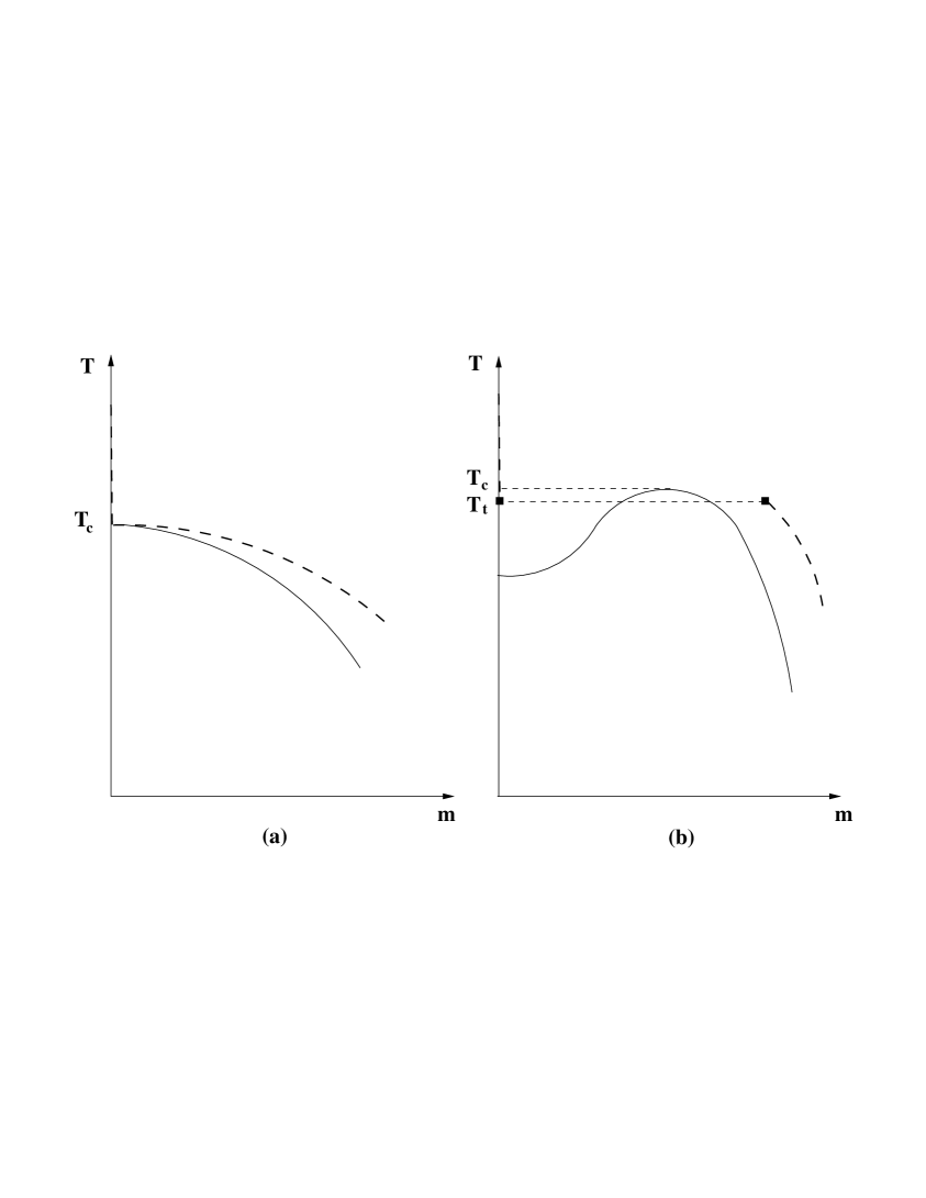
FIG. 1.: Schematic plot of the spinodal curve (solid line) and the spontaneous magnetization versus temperature (dashed line) for second-order (a) and first-order (b) transitions.

FIG. 2.: Spinodal curve (solid line) and spontaneous magnetization versus temperature (dashed line) for $q=3$ (a) and $q=4$ (b).

FIG. 3.: Latent heat $\Delta e$ on the sc, bcc, and fcc lattices for $2.4\leq q\leq 3$. The solid line is the algebraic fit, $\Delta e\sim 0.275\ (q-2.15)^{1.70}$, of the data for the sc lattice.

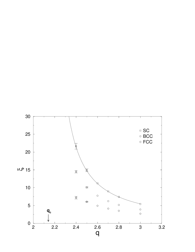
FIG. 4.: Second-moment correlation length on the sc, bcc, and fcc lattices for $2.4\leq q\leq 3$. The solid line is the algebraic fit, $\xi\sim 4.61\ (q-2.14)^{1.14}$, of the data for the sc lattice

FIG. 5.: Coordinates of the critical endpoint in the $T-h$ plane for $q=2.4,2.5,2.6,2.7,2.8,3$, and $3.2$ (from left to right). The corresponding log-log plot indicates that $h_{c}$ vanishes at $k_{B}T_{cc}/(Jc)=0.775\pm 0.003$.

FIG. 6.: Predicted phase diagram of the $q$-state Potts model on the sc lattice. The solid and dashed curves represent the second-order and first-order lines, respectively. The second-order transition occurs in zero field only for $q<q_{c}$. (Note that within numerical accuracy, our results cannot distinguish first from second-order for $2<q<2.4$.)

FIG. 7.: Spinodal curve (solid line) and spontaneous magnetization versus temperature (dashed line) for $q=2$ (a) and $q=1.8$ (b).

FIG. 8.: Log-log plot of the reduced zero-field susceptibility $\chi_{red}=k_{B}T\chi/(q-1)$ versus the reduced temperature $t=1-T_{c}/T$ for $q=2.07,2,1.9,1.8,1.7$ (solid lines from bottom to top) and $q=1.001$ (dashed line).

REFERENCES

- [1] The Laboratoire de Physique Théorique des Liquides is the UMR 7600 of the CNRS.
- [2] R. B. Potts, Proc. Camb. Phil. Soc. 48 (1952) 106.
- [3] F. Y. Wu, Rev. Mod. Phys. 54 (1982) 235; J. Appl. Phys. 55 (1984) 2421.
- [4] T. Kihara, Y. Midzuno, and J. Shizume, J. Phys. Soc. Jpn. 9 (1954) 681.
- [5] R. J Baxter, J. Phys. C. 6 (1973) L445.
- [6] W. Janke and R. Villanova, Nucl. Phys. B B489 (1997) 679 and references therein.
- [7] B. Nienhuis, E. K. Riedel, and M. Schick, Phys. Rev. B 23 (1981) 6055.
- [8] J. B. Kogut and D. K. Sinclair, Solid State Communications 41 (1982) 187.
- [9] J. Lee and J. M. Kosterlitz, Phys. Rev. B 43 (1991) 1268.
- [10] J. S. Hoye and G. Stell, J. Chem. Phys. 67 (1977) 439; Mol. Phys. 52 (1984) 1071; Int. J. Thermophys. 6 (1985) 561.
- [11] R. Dickman and G. Stell, Phys. Rev. Lett. 77 (1996) 996; D. Pini, G. Stell, and R. Dickman, Phys. Rev. E 57 (1998) 2862.
- [12] S. Grollau, E. Kierlik, M. L. Rosinberg, and G. Tarjus, Phys. Rev. E., (in press).
- [13] E. Kierlik, M. L. Rosinberg, and G. Tarjus, J. Stat. Phys. 89 (1997) 215; 94 (1999) 805; 100 (2000) 423.
- [14] J. P. Hansen and I. R. McDonald, Theory of Simple Liquids (Academic, New York, 1976).
- [15] G. S. Joyce, J. of Math. Phys. 12 (1971) 1390; J. Phys. C 4 (1971) L53; J. Phys. A. 5 (1972) L65.
- [16] P. Arnold and Y. Zhang, Nucl. Phys. B 501 (1997) 803.
- [17] N. A. Alves, B. A Berg, and R. Villanova, Phys. Rev. B 43 (1991) 5846.
- [18] A. J. Guttmann and G. Enting, J. Phys. A: Math. Gen. 27 (1994) 5801.
- [19] R. V. Gavai, F. Karsh, and B. Petersson, Nucl. Phys. B 322 (1989) 738.
- [20] R. J Baxter, J. Phys. A.: Math. Gen. 15 (1982) 3329.
- [21] F. Karsch and S. Stickan, Phys. Lett. B 488 (2000) 319.
- [22] I. D. Lawrie and S. Sarbach in: Phase transitions and Critical Phenomena, C. Domb and J. L. Lebowitz Eds. (Academic, London, 1984), Vol. 9.
- [23] P.W. Kasteleyn and E.M. Fortuin, J. Phys. Soc. Japn. Suppl. 26 (1969) 11; Physica 57 (1972) 536.
- [24] D. Stauffer and A. Aharony, Introduction to Percolation Theory (Taylor & Francis, London, 1994).