Acoustic radiation in randomly-layered structures

Abstract

Radiation from acoustic sources located inside randomly-layered structures is studied using the transfer matrix method. It is shown that in contrast to the periodically layered cases where the radiation can be either enhanced or inhibited depending on the frequency, and the characteristics and the material composition of the structures, in the random structures the radiation is always inhibited. The degree of inhibition depends on the acoustic frequency, number of random layers, and the randomness and acoustic parameters of the structures. Both spherically and cylindrically random structures are considered. The results point to the possibility of designing sonic waveguide devices which will not suffer from the energy loss caused by radiation, thus allowing effective energy confinement or long-range energy propagation.

PACS number: 43.20.Fn.

INTRODUCTION

When placed in spatially structured media, the radiation or transmission of optical or acoustic sources will be modulated, a fact of both fundamental importance and practical significance. The structure-modulated transmission, called waveguide propagation, is the backbone of modern opto-electronics and acousto-optics systems. Designing proper waveguide devices that can convey information without or with little energy loss thus has been and continues to be a prime motivation for theoretical studies of wave radiation and propagation in spatially structured media [1].

Much effort has been focused on effects of metal and dielectric interfaces, which can be constructed in either planar, cylindrical, or spherical forms, on optical transmission and radiation [2, 3, 4, 5, 6]. The optical transmission or radiation in periodic structures has attracted particular attention in different areas of applied physics, as in the periodic situations the interaction between propagating waves and structurally periodicity can be either constructive or destructive, leading to significant enhancement or inhibition respectively. In these situations, the waveguides act as a filter which selects particular frequencies for propagation. Understanding of optical propagation in periodicity has been vital to the design of optical devices including optical fibers, semiconductor lasers, hetero-junction bipolar transistors, quantum well lasers, filters, and resonators [1, 6, 7, 8, 9, 10, 11].

Propagation of acoustic waves in spatially structured media has also drawn attention recently [12, 13, 14, 15]. The investigation of acoustic counterparts not only paves the way for the possible design of new acoustic devices, but the acoustic models themselves are advantageous in a number of situations. First, as they are of scalar nature, the acoustic waves are relatively simple to handle yet not to compromise the generality, making them an ideal system for understanding more complicated situations with vector wave propagation. For instance, the recent results on acoustic propagation in water with parallelly placed air-cylinders make it possible to study the ubiquitous phenomenon of wave localization [16] in an unprecedented detailed and manageable manner [15, 17]; the localization of optical waves has posed a long standing problem and a subject of much debate [18]. Second, the research is motivated by potential applications in acousto-optic fiber devices[19]. Third, it is relatively easy to manufacture hetero-structures with large contrast in acoustic impedance. This allows not only the study of strong scattering, but the usage of the properties of the strong scattering in such situations as noise reduction[20].

In the previous paper [15], the acoustic radiation from a source located inside periodically layered spherical cavities has been considered. It is found that significant enhancement or inhibition on the radiation is possible by varying the acoustic parameters and the periodicity of the structures of the guides. The analysis predicts well-defined peaks and nodes in the cavities. The fact that wave transmission in the periodical situations is only possible for certain ranges of frequency is useful as it is of help for devising apparatuses such as filters. For such applications such as energy transport, however, it is desired that no or little energy be radiated for any frequencies. In other words, devices are designed so that energy are confined inside the devices. In this article, we consider acoustic radiation from acoustic sources located inside randomly layered structures. The structures can be of spherical and cylindrical geometries. We show that the radiation is inhibited for all frequencies for any given randomness, and waves are confined in the structures. The confinement or localization effect becomes increasingly significant as the randomness increases or the acoustic contrast increases for a given randomness. These features hold for both spherical or cylindrical structures. The results may be of help in the design of wave processing devices such as resonators or efficient energy guides.

I. FORMULATION OF THE PROBLEM

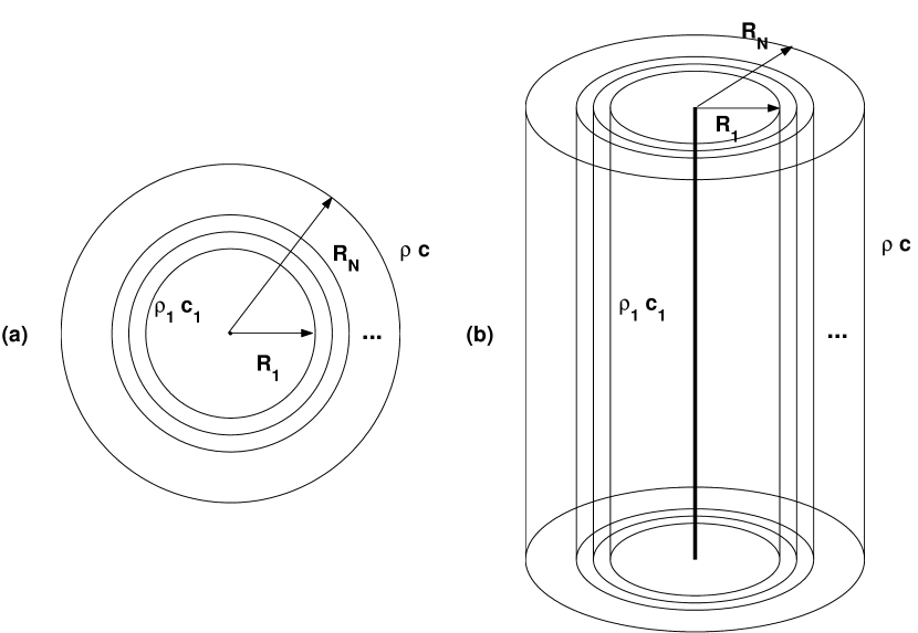
Figure 1: Conceptual layout for spherical and cylindrical cavities.

We consider a unit acoustic source located insider a layered structure, which can be either spherical or cylindrical geometry. The conceptual layout is sketched in Fig. 1. The most inner and outer radii of the structure is $R_{1}$ and $R_{N}$ respectively. Between $R_{1}$ and $R_{N}$, there are $N-1$ randomly placed interfaces. The boundary at $R_{1}$ ($i=1,2,\dots,N$) is denoted as the $i$th interface. These $N-1$ interfaces are randomly located between $R_{1}$ and $R_{N}$. The further parameters are as follows. The sound speed and the mass density inside $R_{1}$ are $c_{1}$ and $\rho 1$, while the sound speed and mass density of the surround medium, i. e. outside $R_{N}$, are denoted by $c$ and and $\rho$ respectively. The sound speed and mass density between the $i$th and the $(i+1)$th interfaces are $c_{i+1},\rho_{i+1}$. We define $g_{i}=\rho_{i}/\rho$ and $h_{i}=c_{i}/c$. The parameters $g_{i}$ and $c_{i}$ are called acoustic contrast parameters.

The Helmholtz wave equation inside the structure is

$$(\nabla^{2}+k_{1}^{2})p(\vec{r})=-4\pi\delta^{(d)}(\vec{r}),\ \ \mbox{for}\ r<R_{1},$$ (1)

where $\nabla^{2}$ is the usual Laplacian operator, $k_{1}$ is the wave number ($k_{1}=\omega/c_{1}$), and $\delta$ is the Dirac delta function representing the source. The superscript $d$ refers to the dimension. For spherical structures, $d=3$, while for cylindrical structures $d=2$. The wave equation outside the structure is

$$(\nabla^{2}+k^{2})p(\vec{r})=0,\ \ \mbox{for}\ r>R_{N},$$ (2)

with $k=\omega/c$. Similarly, the wave equations for the random media between $R_{1}$ and $R_{N}$ are

$$(\nabla^{2}+k_{i}^{2})p(\vec{r})=0,\ \mbox{for}\ i=1,2,3,\dots,N-1,\ \mbox{and}\ R_{i}<r<R_{i+1},$$ (3)

with $k_{i}=\omega/c_{i}$.

Before going into details of the problem we make a detour to consider a more general transmission through an arbitrary interface. The general solution to wave equation such as those in Eqs. (1), (2), and (3) can be written as

$$p_{i}(r)=A_{i}G^{(d)}(k_{i}r)+B_{i}{G^{(d)}}^{\dagger}(k_{i}r),\ (i=1,2,\dots),$$ (4)

where “$\dagger$” means taking the complex conjugate, $A_{i}$ and $B_{i}$ are coefficients to be determined by boundary conditions, and $G^{(d)}$ is the Green’s function in the $d$-th dimension and is written as

$$G^{(d)}(k_{i}r)=\left\{\begin{array}[]{ll}i\pi H_{0}^{(1)}(k_{i}r),&d=2\\ k_{i}\frac{e^{ik_{i}r}}{k_{i}r},&d=3.\end{array}\right.$$ (5)

Note that the Green’s function $G^{(d)}$ also represents the wave transmitted from the unit source without the presence of the layered structures; its complex conjugate represents the inward moving wave.

To solve for the unknown coefficients $A_{i}$ and $B_{i}$, we invoke the boundary conditions that require the pressure field and the radial displacement be continuous across the interfaces. Consider an arbitrary interface at $R$. The wave on the inner ($<$) and outer ($>$) sides of the interface are respectively denoted by

$$p_{<,>}(r)=A_{<,>}G^{(d)}(k_{<,>}r)+B_{<,>}{G^{(d)}}^{\dagger}(k_{<,>}r).$$ (6)

The coefficients $A$ and $B$ on the two sides of the interface can be related by the usual boundary conditions,

$$A_{<}G^{(d)}(k_{<}R)+B_{<}{G^{(d)}}^{\dagger}(k_{<}R)=A_{>}G^{(d)}(k_{>}R)+B_{>}{G^{(d)}}^{\dagger}(k_{>}R),$$ (7)

and

$$\frac{k_{<}}{\rho_{<}}\left[A_{<}{G^{(d)}}^{\prime}(k_{<}R)+B_{<}{G^{(d)}}^{\dagger,\prime}(k_{<}R)\right]=\frac{k_{>}}{\rho_{>}}\left[A_{>}{G^{(d)}(k_{>}R)}^{\prime}+B_{>}{G^{(d)}}^{\dagger,\prime}(k_{>}R)\right],$$ (8)

where “$\prime$” means the derivative, e. g. ${G^{(d)}}^{\prime}(x)=\frac{d}{dx}G^{(d)}(x).$ Eqs. (7) and (8) can be written in the matrix form

$$\left(\begin{array}[]{c}A_{<}\\ B_{<}\end{array}\right)=T(R)\left(\begin{array}[]{c}A_{>}\\ B_{>}\end{array}\right),$$ (9)

with

$$T(R)=\left(\begin{array}[]{cc}G^{(d)}(k_{<}R)&{G^{(d)}}^{\dagger}(k_{<}R)\\ \frac{k_{<}}{\rho_{<}}{G^{(d)}}^{\prime}(k_{<}R)&\frac{k_{<}}{\rho_{<}}{G^{(d)}}^{\dagger,\prime}(k_{<}R)\end{array}\right)^{-1}\left(\begin{array}[]{cc}G^{(d)}(k_{>}R)&{G^{(d)}}^{\dagger}(k_{>}R)\\ \frac{k_{>}}{\rho_{>}}{G^{(d)}}^{\prime}(k_{>}R)&\frac{k_{>}}{\rho_{>}}{G^{(d)}}^{\dagger,\prime}(k_{>}R)\end{array}\right).$$ (10)

The matrix $T$ is called the transfer matrix.

For a system consisting of multiple interfaces, the transmission and reflection coefficients can be related through a consecutive product of the transfer matrices at all the interfaces. We denote the resulting matrix by ${\bf M}$. Therefore, the waves inside and outside the layered structure are related through

$$\left(\begin{array}[]{c}A_{in}\\ B_{in}\end{array}\right)={\bf M}\left(\begin{array}[]{c}A_{out}\\ B_{out}\end{array}\right),$$ (11)

where

$${\bf M}=\prod_{i=1}^{N}T(R_{i})=\left(\begin{array}[]{cc}m_{11}&m_{12}\\ m_{21}&m_{22}\end{array}\right).$$

Now we come back to the problem. Inside the most inner interface, the transmitted wave from the source is subject to reflection from the interface at $R_{1}$. The total wave can be expressed as

$$p(r)=G^{(d)}(k_{1}r)+p_{R}(r),\ \ \mbox{for}\ 0<r<R_{1},$$ (12)

where the first term is the transmitted wave from the source, and the second term is the reflected wave. Since the reflected wave must be finite at the origin, it can be written as

$$p_{R}(r)=-QG^{(d)}(k_{1}r)+Q{G^{(d)}}^{\dagger}(k_{1}r).$$ (13)

The negative sign in front of the first term asserts that the reflected wave remains finite at the origin. Thus the total wave inside the layered structure is

$$p(r)=(1-Q)G^{(d)}(k_{1}r)+Q{G^{(d)}}^{\dagger}(k_{1}r),$$ (14)

which gives $A_{in}=1-Q$ and $B_{in}=Q$. Another observation is that there is no reflected wave outside the layered structure, i. e. beyond $R_{N}$, we have

$$B_{out}=0,\ \ \mbox{for}\ r>R_{N}.$$ (15)

Taking these into consideration, Eq. (11) becomes

$$\left(\begin{array}[]{c}1-Q\\ Q\end{array}\right)=\left(\begin{array}[]{cc}m_{11}&m_{12}\\ m_{21}&m_{22}\end{array}\right)\left(\begin{array}[]{c}A_{out}\\ 0\end{array}\right).$$ (16)

This equation yields the solutions

$$Q=\frac{m_{21}}{m_{11}+m_{21}},\ \ \ A_{out}=\frac{1}{m_{11}+m_{21}}.$$ (17)

¿From these solutions, the radiated acoustic intensity can be computed from

$$I_{out}(r)=\frac{1}{2\rho c}\left(\frac{2\pi}{k}\right)^{3-d}\frac{|A_{out}|^{2}}{r^{d-1}}.$$ (18)

The reflected intensity is

$$I_{R}(r)=\frac{1}{2\rho_{1}c_{1}}\left(\frac{2\pi}{k_{1}}\right)^{3-d}\frac{|Q|^{2}}{r^{d-1}}.$$ (19)

¿From Eq. (14) states that the effective source transmission intensity is

$$I_{s}(r)=\frac{1}{2\rho_{1}c_{1}}\left(\frac{2\pi}{k_{1}}\right)^{3-d}\frac{|1-Q|^{2}}{r^{d-1}}.$$ (20)

Energy conservation states

$$\left(\frac{2\pi}{k_{1}}\right)^{3-d}\frac{1}{\rho_{1}c_{1}}|1-Q|^{2}=\left(\frac{2\pi}{k}\right)^{3-d}\frac{1}{\rho c}|A_{out}|^{2}+\left(\frac{2\pi}{k_{1}}\right)^{3-d}\frac{1}{\rho_{1}c_{1}}|Q|^{2}.$$ (21)

We note some typographical errors about Eqs. (21), (22) and (23) in [14].

We define the transmission (TR) and reflected (RF) coefficients as follows

$$\mbox{TR}=|A_{out}|,\ \ \mbox{RF}=|Q|.$$ (22)

It will become clear that when randomness is added, the transmission will be inhibited for all frequencies. The energy will be confined inside the layered structure. With the random layers, the energy flow in the radial direction decreases as the randomness or the number of layers increases, a useful property for random layered cavities to transport energies.

II. NUMERICAL RESULTS

The situation that the coating layers are periodically placed for spherical cavities has been considered in [14]. For the reader’s convenience, we re-plot the results in Fig. 2. In the computation, the layered structure is constructed as ${\bf A-M-W-M-W-\cdots-W}$, where ${\bf A}$ represents the air inside the cavity, i. e. the air fills the space $r<R_{1}$, ${\bf M}$ refers to the coating material whose acoustic impedance is $\rho_{m}c_{m}$, and $W$ refers to another coating material and we assume it to be similar to that of the surrounding medium, i. e. the water. We define $g=g_{2}=\rho_{m}/\rho$ and $h=h_{2}=c_{m}/c$. Here we take the acoustic contrasts as $\rho_{m}/\rho=2,c_{m}/c=2$. The parameters for air are $\rho_{1}/\rho=0.00129,\ c_{1}/c=0.23$. The horizontal bars represent the interfaces. There are 30 interfaces. The thickness of each layer is set to be identical and equals $0.2R_{1}$; thus the total thickness of the layered materials is $29\times 0.2R_{1}$.

Figure 2 indicates the following. (1) Periodically layered structures selects particular frequencies for transmission, i. e. at these frequencies, the transmission is greatly enhanced. (2) The spectral valleys in which transmission is greatly inhibited are equivalent to the forbidden bands observed in regular lattice solids. These valleys are called forbidden frequency bands. It is known from the previous results that these forbidden bands are caused by Bragg reflection for a periodic structure[14]. (3) The reflection is also significantly enhanced at certain frequencies, and the separation of the reflection peaks is almost constant. (4) It is interesting to see that the results for both spherical and cylindrical geometries are qualitatively similar. The transmission and reflection peaks are only shifted slightly. In the later discussion, we will focus on the results for the cylindrical geometry while the relevant results for the spherical structure will be added only when needed.

Now we consider the randomly layered cases. In the simulation, the layered structures are constructed in the similar way as in the periodical structures, except that the interfaces are randomly placed. To be explicit, the layered structure is ${\bf A-M-W-M-W-\cdots-W}$. There are $N$ interfaces, i. e. there are $N$ horizontal bars. When there is no randomness, the interfaces are equally spaced along the radial direction; the distance between the interfaces is $D=0.2R_{1}$. In this way, the $i$-th interface is located at $r_{i}=R_{1}+(i-1)D$ with $i$ ranging from 1 to $N$. The level of randomness is controlled by the degree of allowing the interfaces to shift from their locations for underlying periodically structures. We define the randomness as $\Delta=\frac{|\delta|}{D}$, where $\delta$ is the range within which the interfaces are allowed to shift from their locations when there are no disorders. For example, the location of the $i$-th interface can be randomly varied with the range between $R_{1}+(i-1)D-\delta$ and $R_{1}+(i-1)D+\delta$. Clearly, the total random is the case that $\Delta=1$.

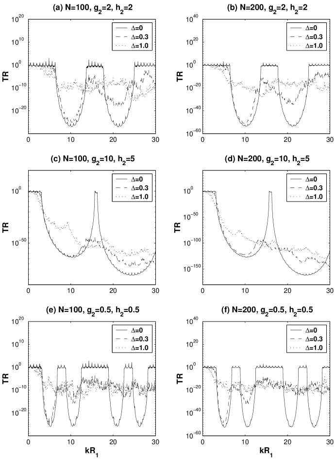
Figure 3: Transmission as a function of frequency in terms of $kR_{1}$ for randomly layered cylindrical structures for various disorders, acoustic contrasts, and numbers of random layers.The results shown are for an arbitrary random configuration.

The effects of the level of randomness, numbers of random layers, and acoustic contrast on the radial transmission are shown in Fig. 3. As both spherical and cylindrical geometries have the similar features, we only plot the results for the cylindrical structures here. The important message from the figure is that when the randomness is added, the transmission is repressed for all frequencies. In other words, no energy can escaped and all energies are confined inside the structure. In particular, Fig. 3 shows the following. (1) When the randomness is introduced, the transmission becomes subdued; when the randomness is small, the band effects from the underlying periodic structures are still noticeable for low frequency bands. This is shown by the case of $\Delta=0.3$. (2) The inhibition is more significant for high frequencies. For the low frequencies, the inhibition seems still possible. This is due to the finiteness in the number of layers. With increasing number of layers, the inhibition will be extended to low frequencies. (3) Fixing the number of layers and when the randomness is greater than a certain value, the effect of the variation in randomness becomes not prominent for high frequencies. This is shown by the tendency that the curves for $\Delta=0.3$ and $1$ merge at high frequencies, referring to the case in, for example, (c) and (e). (4) Increasing the number of random layers, the transmission will be reduced further. In fact, the transmission will decay exponentially with the number of the random layers, as will be shown later. (5) The above features hold when the acoustic parameters vary. (6) For the spherical geometry, we obtain the similar results as in Fig. 3, and because of this we do not show the results here.

With increasing the number of the random layers, the transmission will decrease exponentially. This is illustrated by Fig. 4 for the case $g=h=2$. Here the results are averaged over 200 random configurations. Here is shown the transmission versus the number of random layers for four frequencies and four randomness levels. Out of the four frequencies, two are located at where the transmission is possible when no randomness is introduced, and one is within and one is within but close to the edge of the forbidden band of the underlying periodic structure. It is clear that the increasing randomness decreases gradually the transmission in the regimes in which the transmission is possible when there is no disorder. These regimes may be called the passing bands for the underlying periodical structures. This property is also true for frequencies with but in the vicinity of the forbidden band. Inside the forbidden bands, however, though inhibited the transmission is increased with the added disorder as compared to the case without disorders. This property has also been observed in one-dimensional random liquid media[21, 22]. This indicates that the inhibition due to randomness and the inhibition due to Bragg reflection may have different causes, and the two effects compete. For all frequencies, be within the passing or forbidden bands, the transmission decreases exponentially with increasing numbers of random layers, implying that the most energy is localized near the transmitting source.

The relation between the transmission and the number of layers can be approximately described as

$$I=\frac{I_{0}}{r^{d-1}}e^{-2N/N_{0}}.$$ (23)

The parameter $N_{0}$ represents the effective number of random interfaces to localize the energy, and is named the localization length in terms of the number of interfaces. The localization lengths for the cases in Fig. 4 are summarized in Table 1. It is clear from the table that within the passing bands of the underlying period structure the localization length decreases with increasing frequency and disorders, while well within the forbidden bands the localization length decreases with increasing disorders. This table also shows that the localization lengths are almost identical for the spherical and cylindrical geometries. Moreover, we also see that for the totally random configurations, the energy confinements can be achieved by just a few random interfaces. Further simulation indicates that the localization length decreases with increasing the acoustic contrast.

Table 1: Localization length vs $kR_{1}$ for various randomness $\Delta.$

Spherical Shell                 Cylindrical Shell

$kR_{1}\backslash\Delta$	0.1	0.3	0.5	1.0		0.1	0.3	0.5	1.0
5.5	355.7	42.9	18.0	7.7		390.3	44.2	17.9	7.7
6.0	145.2	20.8	11.0	6.2		143.7	20.4	11.1	6.3
6.5	12.4	8.8	6.9	5.5		12.4	8.8	7.0	5.4
8.0	2.0	2.1	2.7	4.5		2.0	2.1	2.7	4.5

We also examine the reflection behavior. The conservation law in Eq. (21) is rewritten as

$$\left(\frac{2\pi}{k_{1}}\right)^{3-d}\frac{1}{\rho_{1}c_{1}}\left(|1-Q|^{2}-|Q|^{2}\right)=\left(\frac{2\pi}{k}\right)^{3-d}\frac{1}{\rho c}|A_{out}|^{2}.$$ (24)

When the radiation is stopped, i. e. $|A_{out}|\rightarrow 0$, we are thus led to the relation

$$|1-Q|^{2}\approx|Q|^{2}.$$ (25)

The numerical confirmation is shown in Fig. 5, in which the ratio $|1-Q|/|Q|$ is plotted as a function of frequency in terms of $kR_{1}$. With reference to Fig. 2, we see that the ratio deviates from one only for frequencies within the passing bands for the regular structures. With added disorders, this ratio is virtually one for all frequencies. Note that the reason why the ratio is close to one even for the periodic structures is that we take out a term associated with the acoustic impedance.

Finally we note that the results in this papers bear some similarities to the Anderson localization in one dimensional random systems in that no waves can propagate in such a system[21]. The most significant difference is that in the present case, the waves are localized near the transmitting site. In the 1D cases, however, the energy needs not be confined near the source, and there is a stochastic resonance behavior which is absent from the present situations.

III. SUMMARY

In this paper, we consider acoustic radiation from randomly layered cavities. The results in the present paper convey the information that when a cavity is coated by random layers, virtually no energy can be radiated in the radial direction. The waves are mainly localized inside the cavity, and its decay along the radial direction follows an exponential law. The results presented here may be useful for designing acoustic ‘lasers’, resonators, or energy transport. For example, suppose there is a cylindrical wave guide. The propagating wave can be generically written as $e^{ik_{z}z}f(r)$ in the cylindrical coordinates. When the guide is coated by random materials, according to the results, no energy can be radiated into the transverse directions, all energies will be confined inside the guide and can only propagate in the longitudinal direction, i. e. $f(r)$ decreases with $r$. By adjusting the coating materials, the energy transport along the longitudinal axis may be tuned to fit the applications. The results may also be useful for designing possible ‘sonic fibers’ in analogy with the recent all-dielectric optical fibers [6]. For the spherical waveguides, various energies can be stored inside the guides by adjusting the coating materials.

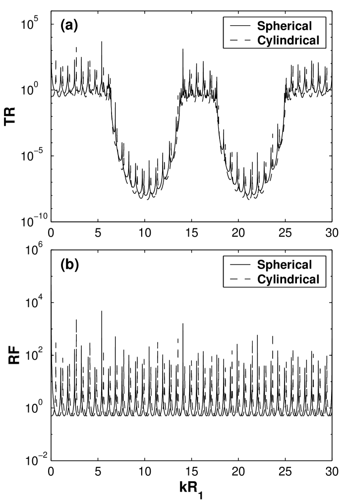
Figure 2: Transmission and reflection coefficients as a function of frequency in terms of $kR_{1}$ for periodically layered cavities: (a) Transmission; (b) Reflection.

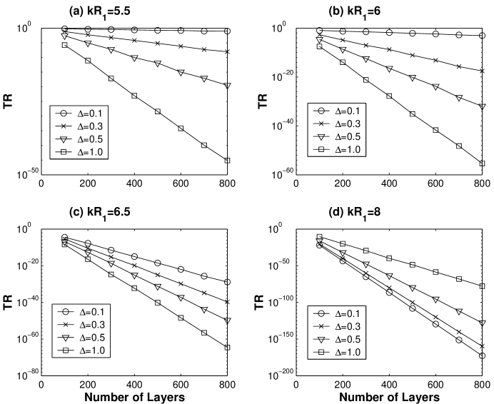
Figure 4: Transmission as a function of the number of random layers for various frequencies and different randomness

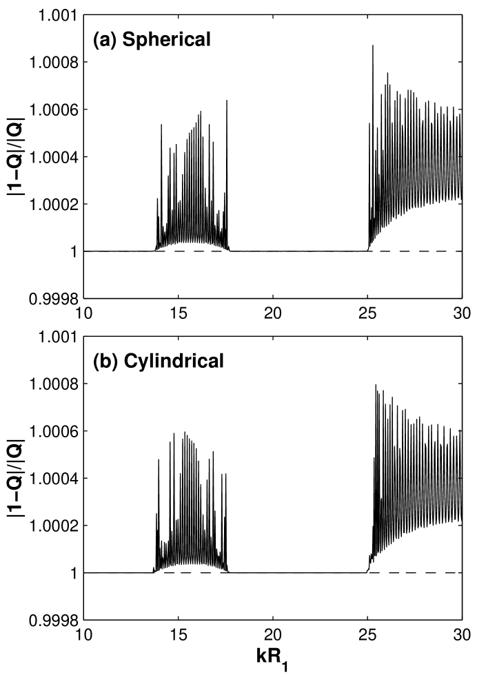
Figure 5: The ratio $|1-Q|/|Q|$ versus $kR_{1}$. The solid and dashed lines are for the periodic and random structures respectively. Here $g=h=2$ and $N=100$

References

- [1] S. E. Miller and A. G. Chynoweth, Eds., Optical Fiber Telecommunications (Academic Press, New York, 1979).
- [2] D. Kleppner, Phys. Rev. Lett. 47, 233 (1981).
- [3] T. Erdogan and D. G. Hall, J. Appl. Phys. 68, 1435 (1990).
- [4] Z. Ye and E. Ping, Solid State Commun. 100, 351 (1996).
- [5] C. C. Wang and Z. Ye, Phys. Status Solidi A 174, 527 (1999).
- [6] M. Ibanescu, Y. Fink, S. Fan, E. L. Thomas, and J. D. Joannopoulos, Science 289, 415 (2000).
- [7] A. Yariv and P. Yeh, Optical Waves in Crystals (John Wiley & Sons, Inc., New York, 1984).
- [8] B. E. A. Saleh and M. C. Teich, Fundamentals of Photonics (Wiley, New York, 1991).
- [9] E. Yablonovitch, Phys. Rev. Lett. 58, 2059 (1987)
- [10] E. Ping and V. Dalal, J. Appl. Phys. 76, 7188 (1994).
- [11] Y. Matsuura and J. Harrington, J. Opt. Soc. Am. 14, 6 (1997), and references therein.
- [12] M. S. Kushwaha, P. Halevi, L. Dovrzynski, and B. Djafari-Rouhani, Phys. Rev. Lett. 71, 2022 (1993).
- [13] M. A. Hawwa, J. Acoust. Soc. Am. 102, 137 (1998).
- [14] Z. Ye, J. Acoust. Soc. Am. 107, 1846 (2000).
- [15] Z. Ye and E. Hoskinson, Appl. Phys. Lett. (in press); cond-mat/0005183.
- [16] e. g. Oxford Consice Dictionary of Science (Oxford Press, New York, 1996).
- [17] E. Hoskinson and Z. Ye, Phys. Rev. Lett. 83, 2734 (1999).
- [18] e. g. F. Scheffold, R. Lenke, R. Tweer, and G. Maret, Nature 398, 206 (1999); D. S. Wiersma, J. G. Rivas, P. Bartolini, A. Lagendijk, and R. Righini, Nature 398, 207 (1999); A. A. Chabanov, M. Stoytchev, and A. Z. Genack, Nature 404, 850 (2000).
- [19] e. g. B. Y. Kim, J. N. Blake, H. E. Engan, and H. J. Shaw, Opt. Lett. 11, 389 (1986); A. Diez, G. Kakarantzas, T. A. Birks, and P. St. J. Russell, Appl. Phys. Lett. 76, 3481 (2000).
- [20] M. S. Kushawha and P. Halevi, Jpn. J. Appl. Phys. 36, L1043 (1997);
- [21] P. G. Luan and Z. Ye, cond-mat/0006006.
- [22] V. D. Frelikher, B. A. Liansky, I. V. Yurkevich, A. A. Maradudin, and A. R. McGurn, Phys. Rev. E 51, 6301 (1995).