Branching and annihilating Lévy flights

Abstract

We consider a system of particles undergoing the branching and annihilating reactions $A\to(m+1)A$ and $A+A\to\emptyset$, with $m$ even. The particles move via long–range Lévy flights, where the probability of moving a distance $r$ decays as $r^{-d-\sigma}$. We analyze this system of branching and annihilating Lévy flights (BALF) using field theoretic renormalization group techniques close to the upper critical dimension $d_{c}=\sigma$, with $\sigma<2$. These results are then compared with Monte–Carlo simulations in $d=1$. For $\sigma$ close to unity in $d=1$, the critical point for the transition from an absorbing to an active phase occurs at zero branching. However, for $\sigma$ bigger than about $3/2$ in $d=1$, the critical branching rate moves smoothly away from zero with increasing $\sigma$, and the transition lies in a different universality class, inaccessible to controlled perturbative expansions. We measure the exponents in both universality classes and examine their behavior as a function of $\sigma$.

I Introduction

Systems possessing a continuous nonequilibrium phase transition from an active into an empty, absorbing state have been intensively studied in the past few years. Despite the wide variety of processes that have been investigated, it has proved possible to classify the critical properties of these transitions into a small number of universality classes. Although the well known case of directed percolation (DP) [1, 2, 3] has turned out to be the most common universality class, many investigations have examined systems with quite different critical properties. For instance, the model of branching and annihilating random walks with an even number of offspring (BARW) defines a separate universality class [3, 4, 5, 6]. This reaction–diffusion system consists of random walkers able to undergo the branching and annihilating reactions $A\to(m+1)A$ and $A+A\to\emptyset$, with $m$ even. Other models in this class (at least in $d=1$) include certain probabilistic cellular automata [7], monomer–dimer models [8, 9, 10], nonequilibrium kinetic Ising models [11], and generalized DP with two absorbing states [12]. These models escape from the DP universality class by possessing an extra conservation law or symmetry. The BARW model respects an additional “parity” conservation of the total number of particles modulo $2$. On the other hand, branching and annihilating random walks with an odd number of offspring possess no such “parity” conservation, and hence belong to the DP universality class[6]. For the other models mentioned above [7, 8, 9, 10, 11, 12], the DP class is escaped via an underlying symmetry between the absorbing states.

Both the DP and BARW classes do, however, share one important feature: the dynamical processes involved are short–ranged. One would expect that the addition of long–ranged processes would significantly alter the properties of the active/absorbing transitions. Recently this expectation was confirmed by investigations of Lévy DP (LDP). This modification, originally proposed by Mollison [13] in the context of epidemic spreading, is a generalization of DP where the distribution of spreading distances $r$ is given by

$$P(r)\sim 1/r^{d+\sigma},\qquad(\sigma>0),$$ (1)

where $d$ is the spatial dimension of the system, and $\sigma$ is a free parameter (the Lévy index) that controls the characteristic shape of the distribution. This distribution is asymptotically (as $r\to\infty$) equal to a Lévy distribution, and we will loosely refer to it as such. It was first suggested that the critical exponents describing the LDP transition should vary continuously with $\sigma$ [14]. This expectation was backed up by field theoretic renormalization group calculations in Ref. [15], and confirmed numerically in Refs. [16, 17]. Note that other numerical work [18, 19] introduced an upper cut off for the flight distance $r$. This resulted in effective short–range behavior, meaning that the LDP regime was not properly accessed. The results of Ref. [19] also appear to be adversely affected by strong finite size effects.

The purpose of the present paper is to further investigate the impact of Lévy flights in models with nonequilibrium phase transitions. We will analyze in detail a model of branching and annihilating Lévy flights with an even number of offspring (BALF), a straightforward generalization of the BARW model, where the random walkers are replaced by particles performing Lévy flights. The BALF model possesses an upper critical dimension $d_{c}$ which varies continuously with the Lévy index $\sigma$. For $d<d_{c}$, the model contains two new universality classes resulting from the long–range nature of the Lévy flights. The exponents in both of these classes also vary continuously with $\sigma$. We will investigate these new universality classes using field theoretic methods, some exact results for the pure annihilation model (where the branching parameter is set equal to zero), and Monte–Carlo simulations in $d=1$.

A further attractive feature of the BALF model is that it casts some additional light on the properties of the ordinary short–ranged BARW model. We will see that changing the Lévy index from $\sigma=1$ to $\sigma=2$ for the BALF model in fixed dimension $d=1$ is in many ways similar to changing the physical dimension from $d=2$ to $d=1$ in the short–ranged BARW model. Although this correspondence is certainly not rigorous, we can nevertheless use simulations of the BALF model in the physical dimension $d=1$ to better understand properties of the BARW model which lie in the inaccessible dimensions between $d=1$ and $d=2$. This will allow us to probe numerically some important features of the BARW field theory developed by Cardy and Täuber in Ref.[6].

We now give a brief summary of the layout of the paper. In the next section we briefly review the relevant properties of the short–ranged BARW model. In Section III we then introduce the BALF model and present its mean field behavior. After these preliminaries we then present the field theoretic action for BALF, which we analyze using diagrammatic and renormalization group methods. These results are then compared with Monte–Carlo simulations in Section IV. Finally, our conclusions appear in Section V.

II Branching and annihilating random walks

The BARW model is defined by the following reaction processes:

$$A\to(m+1)A,\qquad {\rm rate}~{}\mu_{m},$$ (2)

$$A+A\to\emptyset, {\rm rate}~{}\lambda,$$ (3)

where the identical particles $A$ otherwise perform simple random walks with diffusion constant $D$. As the reaction rate parameters are varied, one finds a continuous phase transition from a region controlled by the pure annihilation process to an active region characterized by a nonzero particle density in the steady–state. The growth of BARW clusters close to the critical point can be summarized by a set of independent exponents. A natural choice is to consider $\nu_{\perp}$ and $\nu_{\parallel}$, which describe the divergence of the correlation lengths in space, $\xi_{\perp}\sim|\Delta|^{-\nu_{\perp}}$, and time, $\xi_{\parallel}\sim|\Delta|^{-\nu_{\parallel}}$, close to criticality. Here the parameter $\Delta$ describes the deviation from the critical point at the active/absorbing transition. We also need the order parameter exponent $\beta$, which can be defined in two a priori different ways: it is either governed by the probability that a cluster grown from a finite seed never dies,

$$P(t\to\infty,\Delta)\sim\Delta^{\beta_{\rm seed}},\qquad\Delta>0,$$ (4)

or by the coarse-grained density of active sites in the steady state,

$$n(\Delta)\sim\Delta^{\beta_{\rm dens}},\qquad\Delta>0.$$ (5)

These exponents can be simply calculated in mean field theory, valid for $d>d_{c}=2$. The appropriate mean field rate equation for the coarse–grained density $n({\bf x},t)$ is given by

$$\partial_{t}n=D\nabla^{2}n+m\mu_{m}n-2\lambda n^{2}.$$ (6)

For $\mu_{m}=0$ no branching is present, and we are reduced to the well known annihilation reaction $A+A\to\emptyset$, which asymptotically exhibits a power law mean field density decay $n\sim t^{-1}$. However, for nonzero $\mu_{m}$, we have the homogeneous steady–state solution $n_{s}=m\mu_{m}/2\lambda$. Hence the critical value of $\mu_{m}$ clearly lies at zero, and we identify $\Delta=m\mu_{m}$. The density thus behaves as $n_{s}\propto\Delta$, and we immediately see that $\beta^{MF}_{\rm dens}=1$. The alternative order parameter exponent $\beta_{\rm seed}^{MF}$ can also be simply calculated: for $d>d_{c}=2$, the survival probability (4) of a particle cluster will be finite for any value of the branching rate, implying that $\beta^{MF}_{\rm seed}=0$. This result follows from the non–recurrence of random walks in $d>2$. The correlation length exponents can also be simply derived from Eq. (6), yielding $\nu_{\perp}^{MF}=1/2$, $\nu_{\parallel}^{MF}=1$. Hence the dynamic exponent $z$, defined by $\xi_{\perp}\sim\xi_{\parallel}^{1/z}$, is given by $z^{MF}=\nu_{\parallel}^{MF}/\nu_{\perp}^{MF}=2$.

Below the upper critical dimension the above mean field analysis breaks down due to the presence of fluctuations. Recently, methods have been developed to systematically include these fluctuation effects. Firstly, the appropriate master equation, which provides a complete description of the microscopic dynamics of the system, is transformed into a second–quantized Hamiltonian. This representation is then mapped onto a coarse–grained field theoretic action [20, 21, 22]. From this point the standard tools of renormalized perturbation expansions can be employed, and the effects of fluctuations systematically computed. For the case of BARW, this analysis was performed in Ref. [6]. In the following we summarize the main results of that analysis. The field theoretic action for BARW, written in terms of the response field $\hat{\psi}({\bf x},t)$ and the “density” field $\psi({\bf x},t)$, is given by [6]

$$S_{0}[\psi,\hat{\psi};\tau]=\int d^{d}x\bigg{[}\int_{0}^{\tau}dt\Big{[}\hat{\psi}({\bf x},t)[\partial_{t}-D{\bf\nabla}^{2}]\psi({\bf x},t)$$ (7)

$$\qquad\qquad\qquad\qquad\qquad\quad-\lambda[1-\hat{\psi}({\bf x},t)^{2}]\psi({\bf x},t)^{2}$$ (8)

$$\qquad\qquad\qquad\qquad\quad+\mu_{m}[1-\hat{\psi}({\bf x},t)^{m}]\hat{\psi}({\bf x},t)\psi({\bf x},t)\Big{]}$$ (9)

$$\qquad\qquad\qquad\qquad\qquad\quad-\psi({\bf x},\tau)-n_{0}\hat{\psi}({\bf x},0)\bigg{]}.$$ (10)

Here the terms on the first line of (8) represent diffusion of the particles (with continuum diffusion constant $D$). The second line describes the annihilation reaction (with continuum rate $\lambda$), while the terms on the third line represent the branching process (with continuum rate $\mu_{m}$). The final two terms represent, respectively, a contribution due to the projection state (see Ref. [20]), and the initial condition (an uncorrelated Poisson distribution with mean $n_{0}$). In the following we will restrict ourselves to the case of even $m$, since it is known that the odd $m$ case belongs to the DP universality class [6].

The action given in (8) is a bare action. In order to properly include fluctuation effects one must be careful to include processes generated by a combination of branching and annihilation. In other words in addition to the process $A\to(m+1)A$, the reactions $A\to(m-1)A$, …, $A\to 3A$ need to be included. These considerations lead to the full action

$$S[\psi,\hat{\psi};\tau]=\int d^{d}x\bigg{[}\int_{0}^{\tau}dt\Big{[}\hat{\psi}({\bf x},t)[\partial_{t}-D{\bf\nabla}^{2}]\psi({\bf x},t)$$ (11)

$$\qquad\qquad\qquad+\sum_{l=1}^{m/2}\mu_{2l}[1-\hat{\psi}({\bf x},t)^{2l}]\hat{\psi}({\bf x},t)\psi({\bf x},t)$$ (12)

$$\qquad\quad-\lambda[1-\hat{\psi}({\bf x},t)^{2}]\psi({\bf x},t)^{2}\Big{]}-\psi({\bf x},\tau)-n_{0}\hat{\psi}({\bf x},0)\bigg{]}.$$ (13)

Notice also that (for even $m$) the action (12) is invariant under the “parity” transformation

$$\hat{\psi}({\bf x},t)\to-\hat{\psi}({\bf x},t),\qquad\psi({\bf x},t)\to-\psi({\bf x},t).$$ (14)

This symmetry corresponds physically to particle conservation modulo $2$. The presence of this extra symmetry now takes the system away from the DP universality class, and into a new class: that of branching and annihilating random walks with an even number of offspring.

Simple power counting on the action in Eq. (12) reveals that the upper critical dimension is $d_{c}=2$. Close to $d_{c}$, the renormalization of the above action is quite straightforward (here we again quote the results from Ref. [6]). At the annihilation fixed point the RG eigenvalue of the branching parameter can easily be computed. To one loop order one finds $y_{\mu_{m}}=2-m(m+1)\epsilon/2+O(\epsilon^{2})$, where $\epsilon=2-d$. Hence we see that the lowest branching process is actually the most relevant. Therefore, close to $2$ dimensions where the branching remains relevant, we expect to find an active state for all nonzero values of the branching (in agreement with the mean field theory presented above). Furthermore, in this regime, we can exploit the fact that the critical point, which remains at zero branching, is described by the pure annihilation theory. Matching the exactly known density decay [21] and survival probability exponents in the annihilation theory with their counterparts in the critical BARW theory yields the exact exponent relations $\beta_{\rm dens}=d\nu_{\parallel}/2$, $\beta_{\rm seed}=\nu_{\parallel}(2-d)/2$, and $z=2$ [6]. To the best of our knowledge, the result for $\beta_{\rm seed}$, although simple to derive, has not previously been given in the literature.

Inspection of the one loop result for the most relevant RG eigenvalue $y_{\mu_{2}}$ shows that it eventually becomes negative. This occurs at a second critical dimension $d_{c}^{\prime}$, where $d_{c}^{\prime}=4/3$ to one loop order. For $d<d_{c}^{\prime}$ we expect a major change in the behavior of the system, since the branching process will no longer be relevant at the annihilation fixed point. The critical transition point is then shifted with the active state only being present for values of the branching greater than some positive critical value. For branching parameter values smaller than this value, the branching will be asymptotically irrelevant. This region of parameter space will thus be controlled by the annihilation fixed point of the $A+A\to\emptyset$ process, where the density decays away as a power law. Hence this region of parameter space should be considered a critical inactive (or absorbing) phase. The presence of a second critical dimension $d_{c}^{\prime}\approx 4/3$ immediately rules out any possibility of using perturbative $\epsilon$ expansions to access the non–trivial active/absorbing transition expected in the physical dimension $d=1$. Instead cruder techniques (such as the loop expansion in fixed dimension) must be employed [6]. We will not discuss this part of the analysis of Ref. [6] in much detail. However we do wish to point out that the truncated loop expansion at one loop does predict a jump in the critical point at around $d_{c}^{\prime}\approx 4/3$, from zero branching to some finite value. We will have more to say about his observation in Section IV, after we have presented our analytical and numerical study of the BALF model.

It is also possible to analyze the BARW model in $d=1$ using exact methods. In Ref. [6] it was demonstrated that, at the annihilation fixed point, the one loop RG eigenvalue $y_{\mu_{2}}$ is actually exact in $d=1$. However, the reason for the cancellation of the contributions from higher loop orders in the field theory remains unclear. Other work [23, 24], using quantum spin Hamiltonians, has indicated that the exponents $\beta_{\rm dens}$ and $\beta_{\rm seed}$ are exactly equal at the active/absorbing transition in $d=1$. This conclusion is also supported by numerical simulations [25].

III Branching and annihilating Levy flights

We now turn to the main object of this paper: a systematic investigation of the BALF model. To begin with, we consider the model at the mean field level. The appropriate mean field equation is given by

$$\partial_{t}n=(D_{N}\nabla^{2}+D_{A}\nabla^{\sigma})n+m\mu_{m}n-2\lambda n^{2},$$ (15)

where $D_{N}$ and $D_{A}$ are the rates for normal and anomalous (Lévy) diffusion, respectively. The anomalous diffusion operator $\nabla^{\sigma}$ describes moves over long distances and is defined by its action in momentum space

$$\nabla^{\sigma}e^{i{\bf k}\cdot{\bf x}}=-k^{\sigma}e^{i{\bf k}\cdot{\bf x}},$$ (16)

where $k=|{\bf k}|$. The standard diffusion term $D_{N}\nabla^{2}$ takes into account the short–range component of the Lévy distribution. A more detailed derivation and justification for the Lévy term can be found in Ref. [17]. The mean field exponents can now easily be extracted. The critical point remains at zero branching, and, for $\sigma<2$, we identify $\beta_{\rm dens}^{MF}=1$, $\beta_{\rm seed}^{MF}=0$, $\nu_{\parallel}^{MF}=1$, and $\nu_{\perp}^{MF}=1/\sigma$. Note that, for $\sigma>2$, these exponents cross over smoothly to the ordinary mean field BARW exponents. Even at the mean field level, we can see that the exponent $\nu_{\perp}$ varies continuously with the Lévy index $\sigma$.

The above mean field description will only be quantitatively valid above the upper critical dimension. For $d\leq d_{c}$, we must again take fluctuation effects into account. This can be done using the same methods as were used for the short–ranged BARW model [6]. We emphasize that the inclusion of the long–ranged Lévy processes does not introduce any particular difficulties for the field theory mapping (see Ref. [17] for further details). Specializing immediately to the case with $m=2$, and defining $\mu\equiv\mu_{2}$, we find that the field theoretic action is given by

$$\qquad\qquad\qquad\qquad\qquad S[\psi,\hat{\psi};\tau]=$$ (17)

$$\quad\int d^{d}x\bigg{[}\int_{0}^{\tau}dt\Big{[}\hat{\psi}({\bf x},t)[\partial_{t}-D_{N}{\bf\nabla}^{2}-D_{A}{\bf\nabla}^{\sigma}]\psi({\bf x},t)$$ (18)

$$\qquad\qquad\qquad\qquad\quad-\lambda[1-\hat{\psi}({\bf x},t)^{2}]\psi({\bf x},t)^{2}$$ (19)

$$\qquad\qquad\qquad\quad+\mu[1-\hat{\psi}({\bf x},t)^{2}]\hat{\psi}({\bf x},t)\psi({\bf x},t)\Big{]}$$ (20)

$$\qquad\qquad\qquad\qquad\quad-\psi({\bf x},\tau)-n_{0}\hat{\psi}({\bf x},0)\bigg{]}.$$ (21)

This action describes both normal and anomalous diffusion. The naive scaling dimensions of the fields are

$$[{\hat{\psi}}({\bf x},t)]=\kappa^{0}\,,\quad[\psi({\bf x},t)]=\kappa^{d}\ .$$ (22)

With $[x]=\kappa^{-1}$ and $[t]=\kappa^{-\sigma}$, we see that the naive scaling dimensions of the couplings are

$$[D_{N}]=\kappa^{\sigma-2}\,,\quad[D_{A}]=\kappa^{0}\,,\quad[\lambda]=\kappa^{\sigma-d}\,,\quad[\mu]=\kappa^{\sigma}\ .$$ (23)

Hence, power counting reveals that the upper critical dimension, at which the fluctuations become important, is $d_{c}=\sigma$, for $\sigma<2$.

We have calculated the renormalization group flow functions and eigenvalues, so as to determine the long distance and late time behavior of this field theory. The one loop contribution to the renormalized annihilation vertex is given by the diagram in Fig. 1a. For the case where $\mu=0$, the propagator is $(s+D_{N}k^{2}+D_{A}k^{\sigma})^{-1}$ in $({\bf k},s)$ space ($s$ is the Laplace transformed time variable), or $e^{-(D_{A}k^{\sigma}+D_{N}k^{2})t}$ in $({\bf k},t)$ space. It turns out to be easiest to calculate an extended–time vertex function in $({\bf k},t)$ space, and then determine the renormalized coupling in $({\bf k},s)$ space by performing a Laplace transform and evaluating at the normalization point $({\bf k},s)=({\bf 0},2D_{A}\kappa^{\sigma})$.

FIG. 1.: One loop contribution to (a) the renormalized annihilation vertex and (b) the renormalized branching vertex.

The first step is to drop the normal diffusion term, as it is less relevant for $\sigma<2$. The dimensionless renormalized annihilation coupling is defined by

$$\ell=Z_{\lambda}\lambda C_{d}\kappa^{-\epsilon}/D_{A},$$ (24)

with $\epsilon=d_{c}-d=\sigma-d$, and

$$C_{d}={{\Gamma(d/\sigma)}\over{\Gamma(d/2)}}{{\Gamma(2-d/\sigma)}\over{2^{d-1}\pi^{d/2}}}.$$ (25)

The one loop renormalization factor $Z_{\lambda}$ is then

$$Z_{\lambda}=1-{\lambda\over D_{A}}\frac{C_{d}\kappa^{-\epsilon}}{\epsilon}.$$ (26)

Hence the $\beta$ function is given by

$$\beta_{\ell}(\ell)\equiv\kappa{{\partial\ell}\over{\partial\kappa}}=\ell(d-\sigma+\ell),$$ (27)

with fixed points at $\ell=0$ and $\ell=\ell^{*}=\epsilon=\sigma-d$. The result (27) is actually exact to all orders in perturbation theory [21]. For $d>\sigma$, the Gaussian fixed point at $\ell=0$ is stable, while for $d<\sigma$, the non–trivial $O(\epsilon)$ fixed point at $\ell=\ell^{*}$ is stable.

To investigate the relevance of the branching process, we now calculate the one loop RG eigenvalue for the branching process at the annihilation fixed point. Defining the dimensionless renormalized branching rate as

$$s=Z_{\mu}\mu\kappa^{-\sigma}/D_{A},$$ (28)

then, from the diagram in Fig. 1b, we can compute the one loop renormalization factor

$$Z_{\mu}=1-3{{\lambda}\over{D_{A}}}{{C_{d}\kappa^{-\epsilon}}\over{\epsilon}}.$$ (29)

Hence the $\zeta$ function is

$$\zeta_{\mu}\equiv\kappa{{\partial}\over{\partial\kappa}}\ln{{s}\over{\mu}}=-\sigma+3\ell+{\mathcal{O}}(\ell^{2}).$$ (30)

Thus the one loop RG eigenvalue for the branching process at the annihilation fixed point is

$$y_{\mu}=-\zeta_{\mu}(\ell^{*})=\sigma-3\epsilon=3d-2\sigma.$$ (31)

Consequently, according to the one loop theory, the branching process is relevant at the annihilation fixed point for

$$\sigma<\sigma_{c}^{\prime}(d)=3d/2,$$ (32)

or, in $d=1$, for $\sigma<\sigma_{c}^{\prime}(d=1)=3/2$. Hence, as in the mean field case, we expect an active phase for all nonzero values of the branching rate $\mu$, for sufficiently small $\sigma$ (see also the phase diagram in section IV). In this regime, we can again exploit the fact that criticality lies at zero branching, and hence that the critical behavior of the BALF model coincides with that for the simple Lévy annihilation model $A+A\to\emptyset$ [17]. For the Lévy annihilation model, several exact results can be derived: the density decays as $t^{-d/\sigma}$ (for $d<\sigma<2$) [17]; the survival probability decays as $t^{d/\sigma-1}$ (also for $d<\sigma<2$); and the dynamic exponent is just $z=\sigma$ (for $\sigma<2$). The second of these results follows in a simple way from the analysis of Ref. [26], but is nevertheless, to the best of our knowledge, a new result. On the other hand in the BALF model it is straightforward to show that, at criticality, the density should decay as $t^{-\beta_{\rm dens}/\nu_{\parallel}}$, and the survival probability as $t^{-\beta_{\rm seed}/\nu_{\parallel}}$, and where again we have $z=\sigma$ at the Lévy annihilation fixed point [17]. Matching these results to the Lévy annihilation case, we have $\beta_{\rm dens}=d\nu_{\parallel}/\sigma$ and $\beta_{\rm seed}=\nu_{\parallel}(\sigma-d)/\sigma$.

Hence, in the regime $\sigma<\sigma_{c}^{\prime}(d)$, there is just one independent exponent which must be calculated perturbatively. Following a similar analysis to that in Ref. [6], this exponent can be taken to be $\nu_{\perp}$, which in terms of the RG eigenvalue for the branching is given by $\nu_{\perp}=1/y_{\mu}$. Ideally, at the annihilation fixed point in $d=1$, one would like to be able to calculate the RG eigenvalue $y_{\mu}$ exactly, as was done in the short–ranged BARW model [6]. Remarkably in that case it was found that the one loop result was exact. Unfortunately, generalizing the methods of Ref. [6] to the Lévy case does not seem to be straightforward. However there is some numerical evidence (to be presented in the next section) to suggest that the one loop result for $y_{\mu}$ in the Lévy case is again exact.

We also note that, in the above regime, if $\sigma=2<\sigma_{c}^{\prime}$ then, to one loop order, we expect a smooth crossover to the short–ranged BARW model. Hence, at least at the one loop level, the model in this regime is more straightforward than the LDP case, where there are additional complications (see Refs. [15, 17] for more details).

We now discuss the case where, for $\sigma>\sigma_{c}^{\prime}(d)$, the branching becomes irrelevant at the Lévy annihilation fixed point. For this regime to be present at all, then from Eq. (32), we require $d<4/3$ to one loop order. In this regime we expect the critical branching rate $\mu_{c}(\sigma,d)$ to become nonzero. For $0<\mu<\mu_{c}(\sigma,d)$, the branching will be asymptotically irrelevant, and this phase will again be governed by the exponents of the pure Lévy annihilation universality class [17]. At $\mu=\mu_{c}(\sigma,d)$ we then expect a non–trivial transition to an active phase. As was the case for the short–ranged BARW model we expect this transition to be inaccessible to controlled perturbative expansions, and in a different universality class to that discussed above. This follows from the fact that this transition only appears below a second critical dimension $d<d_{c}^{\prime}(\sigma)=2\sigma/3$ to one loop order. Hence, as was the case for the short–ranged BARW model, $\epsilon=d_{c}-d$ expansions down from the upper critical dimension $d_{c}=\sigma$ will not be able to access this transition.

We note that a “precursor” of the critical inactive phase present for $\sigma>\sigma_{c}^{\prime}(d)$ is already evident in the $\sigma<\sigma_{c}^{\prime}(d)$ regime. Using the above analysis we see that $\beta_{\rm dens}=d/y_{\mu}=d/(3d-2\sigma)$ for $\sigma<\sigma_{c}^{\prime}(d)$ (to one loop). Hence, to this order, as $\sigma\to\sigma_{c}^{\prime}(d)=3d/2$ from below, $\beta_{\rm dens}$ diverges. This implies that for a fixed small value of the branching, the active phase has a decreasing density as a function of $\sigma$, as $\sigma$ is increased towards $\sigma_{c}^{\prime}(d)$. Finally at $\sigma=3d/2$ (to one loop order) an entire critical inactive phase opens up.

We can now see the similarities between properties of the short–ranged BARW model as dimension is lowered from $d=2$ to $d=1$, and the BALF model in $d=1$, as the Lévy index is raised from $\sigma=1$ to $\sigma=2$. In particular, to one loop order, the region $1<\sigma<\sigma_{c}^{\prime}(d=1)=3/2$ for the $d=1$ BALF model contains the direct analog of the inaccessible universality class present in BARW for $d_{c}^{\prime}\approx 4/3<d<2$.

IV Simulation results

In order to further investigate the BALF universality class, we have performed extensive numerical simulations of a lattice BALF model in $d=1$. At each time step, a randomly chosen particle was allowed either to branch, with probability $1-p$, or to move, via a long–range jump, with probability $p$; $p$ was the only parameter in the simulations. The number of particles at each lattice site was restricted to zero or one: thus, when a particle moved to an occupied site, both particles were annihilated. At each branching step, a particle produced two offspring, which occupied the two sites to the immediate left or right of the original particle, with the side chosen randomly. As pointed out in Ref. [27], this method of choosing occupied sites is necessary since if the newly occupied sites are chosen symmetrically about the original site, then the short–ranged BARW model turns out to be in its inactive state for all $0<p\leq 1$.

The distribution of hop lengths was chosen to follow Eq. (1), for $r\geq 1$. This distribution is implemented by choosing a random number $x$ from a uniform distribution on the interval $[0,1)$, and then calculating a new random variable $r=(1-x)^{-1/\sigma}$. It is easy to see that this produces a sequence of numbers whose distribution follows Eq. (1).

Two different initial conditions were used to calculate the different exponents. In the first case, the initial condition was a “seed” of two particles at lattice sites $\pm 1$. See Fig. 2 for some sample runs with this initial condition, run for $500$ time steps. The long–range hops at small $\sigma$ result in a very rapid and wide–ranging dispersal of the particles.

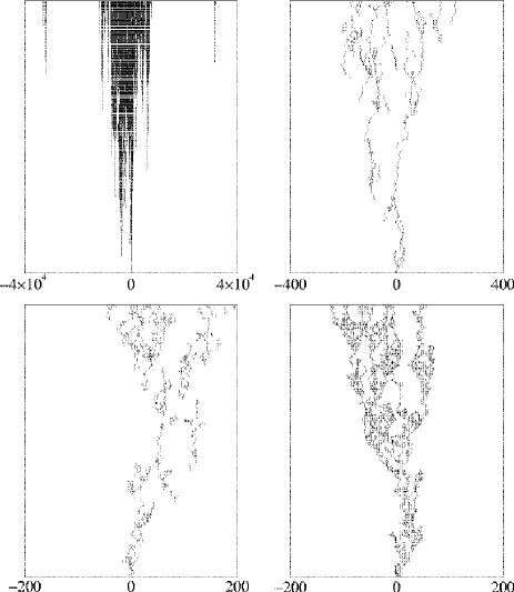
FIG. 2.: Sample runs at various values of $\sigma$, with time evolution running up the page. All runs are for $500$ time steps, and are at values of $p$ about $10\%$ away from the critical point into the active phase. The top two frames show $p=0.9$, at $\sigma=1.0$ and $\sigma=1.5$, from left to right. The lower left frame shows $\sigma=1.9$, $p=0.77$, and the lower right frame shows the ordinary short–ranged BARW model at $p=0.46$. Notice the large change in scale between the first and last frame.

These simulations were averaged over many runs from the same initial condition but for different sequences of random numbers. The number of runs, $P(t)$, surviving to time $t$, the number of particles in the system averaged over the total number of runs, $N(t)$, and a mean square spreading distance, $R^{2}(t)$, were all measured. The mean spreading distance is defined by a geometric mean in the Lévy case (see Ref.[17] for more details). At the critical point, these quantities should all follow power law behavior with

$$P(t)\sim t^{-\delta},$$ (33)

$$N(t)\sim t^{\theta},$$ (34)

$$R^{2}(t)\sim t^{2/z}.$$ (35)

The critical point is determined by plotting a local exponent against $1/t$, and estimating the value of $p$ which produces a straight line as $1/t\rightarrow 0$. For the survival probability, the local exponent is defined by

$$-\delta(t)={{\ln{{P(t)}\over{P({{t}\over{b}})}}}\over{\ln b}},$$ (36)

and similarly for the other quantities. We have used $b=5$ in our data analysis. The extrapolation of the exponent to $1/t\to 0$ is the estimate of its long time value. A sample analysis, for $\sigma=1.6$, is shown in Fig. 3.

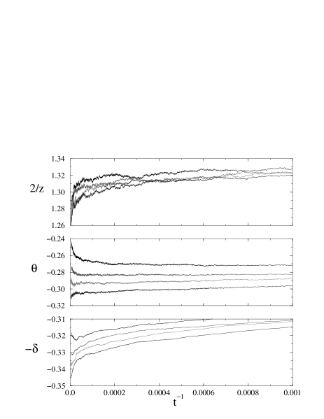
FIG. 3.: The effective local exponents, as in Eqs. (33)-(35), for $\sigma=1.6$. The exponents are plotted against $1/t$ to extract the $t\rightarrow\infty$ limit. The curves correspond to values of $p$, from top to bottom, of $0.985$, $0.988$, $0.99$, and $0.992$.

We focus first on the perturbatively inaccessible transition found for larger values of $\sigma>\sigma_{c}^{\prime}(d=1)$. In this regime we performed simulations at criticality and measured the exponents defined in Eqs. (33)-(35). To reduce finite size effects, we implemented periodic boundary conditions and used a very large lattice. Rather than store the occupation numbers of each lattice site, only the positions of the particles were stored. This meant that the system size was limited only by the number of integers, i.e. a system size of $2^{64}\approx 1.8\times 10^{19}$ on the $64$–bit computer used. The simulations ran for times of between $2\times 10^{4}$ and $2\times 10^{5}$ time steps per particle, and were averaged over at least $2\times 10^{6}$ runs.

We encountered several obstacles in accurately determining the values of these exponents. First, the quantities measured were also expected to behave as power laws on the (critical) inactive side of the transition. The difference between the equivalent exponents on the critical line and in the critical phase were sometimes small, particularly near $\sigma=\sigma_{c}^{\prime}(d=1)$, where the fixed point we investigated merges with the pure Lévy annihilation fixed point. Consequently measurements close to this point required the longest runs. Also, corrections to scaling meant that the effective local exponents did, in fact, vary with $t$. The impact of these corrections to scaling was sometimes difficult to interpret accurately. Finally, the various exponents measured yielded slightly different estimates for $p_{c}$, making it difficult to determine the critical point more accurately than done here. This may be due to the corrections to scaling being of different sizes for each of the exponents measured.

The results of these simulations are shown in Table I. The $\sigma=\infty$ values shown are for simulations with normal diffusion, where the exponents measured are consistent with those of other simulations [5, 27]. Fig. 4 shows the phase diagram as determined by the simulations.

We now discuss some features of the numerical data in Table I:

$\bullet$ The data presented in Table I is consistent with a value very close to $\sigma=\sigma_{c}^{\prime}(d=1)=3/2$ for the emergence of the critical Lévy annihilation phase at nonzero branching. This is in good agreement with the one loop result for $y_{\mu}$ in Eq. (31), and provides some evidence that this one loop result may in fact be exact, as it was for the short–ranged Lévy case.

$\bullet$ The measured exponents changed by rather small amounts over the range of $\sigma$ studied. As discussed in section III, the exponents at $\sigma=\sigma_{c}^{\prime}(d=1)$, $p=1$, can be calculated for the pure Lévy annihilation model, and, assuming $\sigma_{c}^{\prime}(d=1)=3/2$, are given by $\delta=-\theta=1/3$, $z=3/2$. If the exponents are to change monotonically as $\sigma$ is varied, then they are trapped in a relatively small range of values between the BARW and Lévy annihilation exponents.

$\bullet$ The numerical evidence also strongly favors a smooth movement of the critical value $p_{c}$ away from unity as $\sigma$ is increased above $3/2$, as shown in Fig. 4. This finding has consequences for the analogous short–ranged BARW model. In that case the analog of the point at $\sigma=\sigma_{c}^{\prime}(d=1)\approx 3/2$ is the second critical dimension found at $d_{c}^{\prime}\approx 4/3$. The uncontrolled truncated loop expansion used to analyze this point in Ref. [6] predicted a discontinuous jump of the critical point as dimension $d$ is lowered through $d_{c}^{\prime}$. The above numerical evidence argues against this scenario and would rather predict a smooth movement of the critical point. Given the uncontrolled nature of the truncated loop expansion, any failure to accurately capture the behavior close to $d_{c}^{\prime}$ would not, perhaps, be very surprising. Nevertheless, our results have, for the first time, provided numerical evidence for one of the main conclusions of Ref. [6], namely the presence of a second critical dimension $d_{c}^{\prime}$.

$\bullet$ Despite considerable effort, the data reported in Table I are unfortunately not precise enough to answer the question: at what value of $\sigma$ do the Lévy results cross over to those of the short–ranged BARW model? Regrettably, the situation from a theoretical perspective is no clearer, due to the absence of any controlled field theoretic methods in this regime.

We now turn our attention to the second regime for $d=1$ BALF, that for $\sigma<\sigma_{c}^{\prime}(d=1)\approx 3/2$. In this case, it is not appropriate to perform simulations at criticality, since in that case we would only be measuring the exponents of the pure Lévy annihilation model. Hence we have performed off–critical simulations in an effort to measure $\beta_{\rm dens}$ as a function of $\sigma$. In this case, we used a second initial condition, a fully occupied lattice of size $L=10^{7}$. We then allowed the number of particles to decay away until a steady–state was reached. The steady–state density depends on the deviation from the critical point, as described by Eq. (5), and thus $\beta_{\rm dens}$ may be directly measured.

FIG. 4.: Phase diagram for the BALF model in $d=1$. The inset shows a blowup of the region near $\sigma_{c}^{\prime}(d=1)$.

$\sigma$	$p_{c}$	$\delta$	$\theta$	$z$
1.525	0.997(2)	0.32(1)	-0.30(1)	1.53(2)
1.55	0.992(4)	0.32(2)	-0.30(2)	1.53(2)
1.6	0.990(2)	0.33(2)	-0.30(2)	1.56(2)
1.65	0.974(2)	0.32(2)	-0.26(2)	1.55(2)
1.7	0.955(2)	0.32(2)	-0.24(2)	1.59(2)
1.8	0.918(2)	0.32(2)	-0.18(2)	1.59(2)
1.9	0.863(2)	0.32(2)	-0.14(1)	1.63(2)
2.0	0.804(1)	0.305(5)	-0.085(5)	1.68(2)
2.5	0.6185(2)	0.285(5)	-0.005(5)	1.72(1)
$\infty$	0.5104(2)	0.287(3)	0.001(3)	1.74(1)

TABLE I.: The measured critical probabilities and exponents for various values of $\sigma$. The number in brackets is an estimate of the error in the last figure.

The values of $\beta_{\rm dens}$ measured in these steady–state simulations are given in Table II. For $\sigma<1$ the mean field result should hold, since $d=1$ then lies above the upper critical dimension $d_{c}=\sigma$. For $\sigma$ slightly bigger than unity, the upper critical dimension will lie just above $d=1$, and hence one might hope to directly observe the $\epsilon$ expansion results (see also Ref. [17] for a similar case). Unfortunately, the values measured in the simulations deviate by around $5-25\%$ from the mean field or one loop $\epsilon$ expansion exponents calculated in section III. We believe there are two reasons for this discrepancy. Firstly, for small $\sigma$, finite size effects become important, as the long–ranged hops allow a single particle to wrap all the way around the system in a short time. Secondly, as $\sigma\rightarrow\sigma_{c}^{\prime}(d=1)\approx 3/2$, $\beta_{\rm dens}$ becomes rather large, and hence large systems and long runs were necessary to probe the very small steady–state densities which occur near $p_{c}$. Although we used as large a system as practicable, we were not able to entirely eliminate the discrepancy between theory and simulations.

In summary, despite the difficulties encountered for $\sigma<\sigma_{c}^{\prime}(d=1)$, the overall picture that emerges from the numerics agrees well with the theory presented in the last section. As we have discussed earlier, this, in turn, provides additional support for the analysis of the short–ranged BARW model presented in Ref. [6].

$\sigma$	$\beta_{\rm dens}$ (measured)	$\beta_{\rm dens}$ (theory)
0.7	1.0	1 (mean field)
0.9	1.1	1 (mean field)
1.1	1.3	5/4 (one loop)
1.3	1.8	5/2 (one loop)

TABLE II.: The exponent $\beta_{\rm dens}$ determined in simulations of the steady–state density of a system of size $10^{7}$.

V Conclusions

In this paper we have presented an analytic and numerical study of the BALF model. Using field theoretic techniques we have obtained a good analytic understanding of the model in the physical dimension $d=1$ for the regime $\sigma$ less than about $3/2$. For values of $\sigma$ larger than this, we have had to rely solely on numerical simulations. In both regimes the critical exponents of the active/absorbing transition are found to vary continuously with the Lévy index $\sigma$. Numerically, we find that the transition between the two regimes in $d=1$ occurs at $\sigma=\sigma_{c}^{\prime}(d=1)\approx 3/2$, in agreement with the one loop result from the field theory. Unfortunately our numerics for the small $\sigma$ regime were not good enough to confirm the accuracy of our $\epsilon$ expansion calculations. Nevertheless this is the first time this universality class has been accessed, since its equivalent in the original BARW model lies in the inaccessible dimensions $d_{c}^{\prime}<d<2$.

Finally, we would like to emphasize that Lévy flights are a powerful way of probing the higher dimensional behavior of nonequilibrium models while performing simulations only in $d=1$. The disadvantage of this approach is that it necessitates the use of extremely large system sizes if finite size effects are to be avoided. However, we have shown that in large regions of parameter space these problems can be overcome, and reasonable estimates obtained for the exponents.

REFERENCES

- [1] W. Kinzel, in Percolation Structures and Processes, edited by G. Deutscher, R. Zallen, and J. Adler, Annals of the Israel Physical Society, Vol. 5 (Adam Hilger, Bristol, 1983).
- [2] P. Grassberger and K. Sundermeyer, Phys. Lett. B 77, 220 (1978); P. Grassberger and A. de la Torre, Ann. Phys. (N.Y.) 122, 373 (1979); J.L. Cardy and R. L. Sugar, J. Phys. A 13, L423 (1980); H.K. Janssen, Z. Phys. B 42, 151 (1981).
- [3] H. Hinrichsen, Adv. Phys. 49, 815 (2000).
- [4] H. Takayasu and A.Yu. Tretyakov, Phys. Rev. Lett. 68, 3060 (1992).
- [5] I. Jensen, Phys. Rev. E 50, 3623 (1994).
- [6] J. Cardy and U.C. Täuber, Phys. Rev. Lett. 77, 4780 (1996); J. Stat. Phys. 90, 1 (1998).
- [7] P. Grassberger, F. Krause, and T. von der Twer, J. Phys. A: Math. Gen. 17, L105 (1984); P. Grassberger, J. Phys. A: Math. Gen. 22, L1103 (1989).
- [8] M.H. Kim and H. Park, Phys. Rev. Lett. 73, 2579 (1994); H. Park, M.H. Kim, and H. Park, Phys. Rev. E 52, 5664 (1995).
- [9] W. Hwang, S. Kwon, H. Park, and H. Park, Phys. Rev. E 57, 6438 (1998).
- [10] W. Hwang and H. Park, Phys. Rev. E 59, 4683 (1999).
- [11] N. Menyhárd and G. Ódor, J. Phys. A 29, 7739 (1996).
- [12] H. Hinrichsen, Phys. Rev. E 55, 219 (1997).
- [13] D. Mollison, J. R. Stat. Soc. B 39, 283 (1977).
- [14] P. Grassberger, in Fractals in physics, eds. L. Pietronero and E. Tosatti (Elsevier, Amsterdam, 1986).
- [15] H.K. Janssen, K. Oerding, F. van Wijland, and H.J. Hilhorst, Eur. Phys. J. B 7, 137 (1999).
- [16] M.C. Marques and A.L. Ferreira, J. Phys. A 27, 3389 (1994).
- [17] H. Hinrichsen and M. Howard, Eur. Phys. J. B 7, 635 (1999).
- [18] E.V. Albano, Europhys. Lett. 34, 97 (1996).
- [19] S.A. Cannas, Physica A 258, 32 (1998).
- [20] L. Peliti, J. Physique 46, 1469 (1985).
- [21] B. Lee, J. Phys. A 27, 2633 (1994).
- [22] J.L. Cardy, in The Mathematical Beauty of Physics, edited by J.-B. Zuber, Advanced Series in Mathematical Physics Vol. 24 (World Scientific, River Edge, NJ, 1997), p.113.
- [23] K. Mussawisade, J.E. Santos, and G.M. Schütz, J. Phys. A 31, 4381 (1998).
- [24] M. Howard, P. Fröjdh, and K. Lauritsen, Phys. Rev. E 61, 167 (2000).
- [25] I. Jensen, J. Phys. A 30, 8471 (1997).
- [26] B.D. Hughes, Physica A 134, 443 (1986).
- [27] S. Kwon and H. Park, Phys. Rev. E 52, 5955 (1995).