Bent surface free energy differences from simulation

Abstract

KEYWORDS: Molecular dynamics, Bending of surfaces, Surface thermodynamics, Gold, Curved Surfaces.

^a SISSA, Trieste, Italy
^b Unitá INFM/SISSA
^c ICTP, Trieste, Italy
^d Max-Planck-Institut f. Festkoerperforschung, Stuttgart, Germany
^† Corresponding author. Address: SISSA, Via Beirut 2, I-34014 Trieste, Italy. FAX: +39-040-3787528. E-mail: tartagli@sissa.it

ECOSS 19 – Abstract number: 00456

KEYWORDS: Molecular dynamics, Bending of surfaces, Surface thermodynamics, Gold, Curved Surfaces.

1 Introduction

The surface free energy of a solid, defined as the excess free energy of the semi-infinite solid relative to an infinite solid with equal number of particles[1], is a very important but also a very elusive quantity. It is important because its minimum determines the surface equilibrium state and its properties. However, while in the liquid it coincides with the ordinary surface tension, in the solid it becomes elusive because there it can neither be easily measured nor calculated. The quantity which is easy to access is instead the surface stress (generally a rank 2 tensor) defined as the change of the surface free energy with respect to a unitary increase of surface area upon stretching, which combines surface specific free energy $\gamma$ and its first derivative:

$$\sigma^{\textrm{\scriptsize(s)}}=\gamma+A\frac{d\gamma}{dA}$$

While $\gamma$ is of course positive for a substance below its critical point, the magnitude of the second term (arising from the rigidity of the solid) is generally comparable, but can have either sign. Therefore, while surface stress is becoming increasingly available through measurement[2], simulation[3], and microscopic calculation[4], the surface free energy remains generally unknown. At $T=0$, where surface free energy and surface energy coincide, there are of course a large number of calculations, as quoted e.g. in Ref. [2]. However, finite temperature free energy calculations, including the entropy term, seem totally missing. This is particularly frustrating in view of the desire to characterize and possibly predict surface phase transitions as a function of parameters, such as temperature, coverage, external stresses, crystal bending, etc. In systems where interatomic forces are well understood, an alternative methods to predict such phase transition is simulation, particularly Molecular Dynamics (MD) simulation. However, besides being somewhat less fundamental, the simulation approach usually suffers from practical problems, such as size and time limitations, which greatly restrict the variety of transitions that can be directly described.

In the present paper we present a route to calculate directly the surface free energy change with respect to one specific external parameter, the curvature of the underlying solid. The method is again based on Molecular Dynamics (MD) simulations, and uses the framework for variable curvature MD developed by Passerone et al.[5]. The surface phases to be compared can be either simulated separately, or realized on the two opposite faces of the same simulation slab. Since free energies are calculated separately, the actual phase transformation is not required to take place spontaneously in the simulation – in fact, it must be avoided. Curvature of a crystal plate is a standard tool for observing surface stress difference of the two opposite faces of the plate[6, 2]. Conversely, inducing curvature of the plate by an external bending force will cause the two opposite faces to depart from their original state, and their free energies will generally evolve in opposite directions.

We have chosen metallic surfaces as our test case, for a variety of reasons. The surfaces of metals are readily accessible to a variety of surface techniques. Especially noble and some transition metals show a variety of surface reconstructions where the surface stress plays an important role[2]. If a metal slab is bent the surfaces are strained and work is exerted onto them. It is plausible that bending could eventually drive phase transitions, including changes or removal of the reconstruction. Preliminary results on reconstructed Au(111) indicate that the surface reconstruction, or at least some features of it, can in fact be removed by curvature[7]

2 Method

Although MD is a very useful technique to study the time evolution of energies, temperature, pressure, stress, …  of a system with well defined forces, other thermodynamic quantities, like the free energy and entropy, are not obtained. The reason is that such quantities are not an average of some mechanical entity over the ensemble of the states: they contain information on the whole ensemble of states which cannot be directly extracted from the time evolution of a sample[8]. Nonetheless in some specific cases the free energy variation along a reversible, isothermal path can be determined from mechanical quantities by integrating the work done onto the system.

In the particular case of the slab, where curvature is forced externally through bending, the work is given by the integral of the stress tensor with respect to the strain and the volume of the slab. This integral contains contributions both from the surfaces and from the bulk of the slab. For our purposes, the former must be separated from the latter[9]. The first step is to extract the total stress field $\sigma_{\alpha\beta}$ in the simulation of a curved slab. The only relevant component is $\sigma_{yy}$, where the $y$-axis is parallel to the surface and is oriented in the direction that is stretched during bending (the other axes are chosen with $z$ normal to the slab). The average force exchanged across the $xy$-plane is[3]

$$T_{yy}\equiv\sigma_{yy}\cdot L_{x}L_{z}=-\frac{1}{L_{y}}\left\langle\sum_{i}\frac{p_{iy}^{2}}{m_{i}}\right\rangle-\frac{1}{2L_{y}}\left\langle\sum_{i,j\>(i\neq j)}\frac{\partial U}{\partial r_{ij}}\frac{(x_{i}-x_{j})^{2}}{r_{ij}}\right\rangle~{},$$ (1)

where the indexes $i$ and $j$ runs over the particles, $U$ is the potential energy as a function of the interatomic distances $r_{ij}\equiv|\vec{r}_{i}-\vec{r}_{j}|$ and $L_{x}$, $L_{y}$, $L_{z}$ indicate the lengths of the slab along the three axes (the latter being the slab thickness). Note that this formula does not require pairwise potentials as it might seem. It applies for arbitrary many body potentials (including EAM, glue models, etc) such that total energy depends only on pair distances. In the following for convenience we shall write $F_{ij}$ in place of $\partial U/\partial r_{ij}$. Note that this is generally not the force acting between particles $i$ and $j$, but it becomes that in the specific case of pairwise additive interactions. The first term in the RHS is the kinetic energy contribution to stress, which in the classical case is just $(Nk_{B}T/V)\cdot L_{x}L_{y}$, being $N$ the number of atoms and $V\equiv L_{x}L_{y}L_{z}$ the volume of the cell. The second term arises from interparticle interactions: it is the derivative of the potential energy with respect to a uniform stretching along the $y$-axis, averaged over the system configurations.

We cut a slab in slices along the $z$ direction, each slice corresponding to one layer (the depth coordinate $z$ is orthogonal to the bending axis $x$, and to the bending direction $y$). By restricting the sum to particles located in each slice we calculate the stress along the bending direction, resolved layer by layer. For a bent slab, equation (1) must be generalized to compute the average stress per layer in the direction which locally follows the profile of the surface. This is done by computing the potential energy derivative for a uniform strain of the slab along y. In order to better deal with the symmetry of the bent slab, we introduce a system of scaled, curved coordinates $(q_{1},q_{2},q_{3})$; indicating with $k$ the slab curvature in the neutral cylinder (i.e.  in the middle of the slab):

$$\left\{\begin{array}[]{l}x=L_{x}q_{1}\\ y=(1/k+L_{z}q_{3})\sin(kL_{y}q_{2})\\ z=(1/k+L_{z}q_{3})\cos(kL_{y}q_{2})-1/k\end{array}\right.$$ (2)

The variable $q_{2}$ is proportional to the polar angle $\theta$ through $\theta=kL_{y}q_{2}$; thus $q_{2}$ moves along the bending direction. The “radial” coordinate $q_{3}$ is measured along the direction normal to the surface and is zero in the middle layer. Each of these coordinates ranges between $-1/2$ and $1/2$. In the limit of zero curvature they are proportional to $x$, $y$ and $z$ respectively and correspond to the scaled coordinates introduced by Andersen[11] and by Parrinello and Rahman[12]. We note that this system of coordinates is slightly different from the one introduce in ref. [5]: the present choice is more convenient in order to compute the stress field. Omitting the details of the calculation, the final formula for the derivative of the potential energy keeping all the scaled coordinates fixed is

$$\frac{\partial U}{\partial L_{Y}}=\frac{1}{2}\sum_{i,j\>(i\neq j)}\left[\frac{F_{ij}}{r_{ij}}(1+q_{3i}kL_{z})(1+q_{3j}kL_{z})\frac{\theta_{ij}\sin(\theta_{ij})}{k^{2}L_{y}}\right]$$ (3)

Since periodic boundary conditions are used, both the distances $r_{ij}$ and the differences $\theta_{ij}\equiv\theta_{i}-\theta_{j}=kL_{y}(q_{2i}-q_{2j})$ must be computed with the minimum image convention. The contribution of particle $i$ to the force $\int\!\!\int\!dxdz\,\sigma_{22}$ is

$$-\frac{k_{B}T}{L_{y}}-\frac{1}{2}\sum_{j\>(j\neq i)}\left[\frac{F_{ij}}{r_{ij}}(1+q_{3i}kL_{z})(1+q_{3j}kL_{z})\frac{\theta_{ij}\sin(\theta_{ij})}{k^{2}L_{y}}\right]$$

The average force any layer exerts in the $q_{2}$ direction is obtained as:

$$T_{22} = -\left\langle N_{\mbox{\scriptsize layer}}\right\rangle\frac{k_{B}T}{L_{y}}-\Bigg{\langle}\sum_{i\in\mbox{\scriptsize layer}}\Bigg{\{}\frac{1}{2}\sum_{j\in\mbox{\scriptsize slab}\>(j\neq i)}\bigg{[}$$ (4)

$$\frac{F_{ij}}{r_{ij}}\,(1+q_{3i}kL_{z})\,(1+q_{3j}kL_{z})\,\frac{\theta_{ij}\sin(\theta_{ij})}{k^{2}L_{y}}\,\bigg{]}\Bigg{\}}\Bigg{\rangle}$$

In the zero curvature limit , $k\to 0$, this formula reduces to (1).

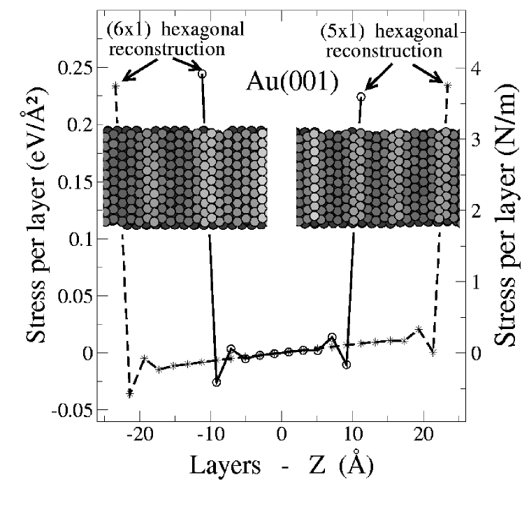
Figure 1: The linear stress (force/length) associated to every layer of two samples with different thicknesses. In the insets the reconstructions of the two surfaces are shown. Surface atoms with the largest $|z|$ are shown as lighter, and identify the reconstruction solitons. Note the bulk linear $z$ dependence, and the large surface contribution.

To exemplify, we apply this scheme to the Au(001) surface, modeled by means of the “glue” many body potential[13]. It is well known that this surface reconstructs with a denser triangular top layer[14, 15], increasing its lateral density by about 24% relative to an unreconstructed layer. One could expect that the tensile stress typical of the unreconstructed surface should have decreased, maybe even disappeared, or reversed. Moreover, different reconstruction periodicities with different lateral densities and different surface stresses might come in competition with one another for the lowest free energy, as curvature is cranked up. Figure 1 shows the stress $T_{22}/L_{x}$ in each slice of a (001) gold slab. The two slab surfaces are given two slightly different reconstructions, namely $1\times 5$ (close to the experimental one) and $1\times 6$ (with slightly lower surface density). Two slab samples are considered: one made by 12 layers and a thicker one made by 24 layers. Both samples have sizes $L_{x}=28.8$Å and $L_{y}=172.9$Å. The bending direction is [110]. The stress is computed through (4) taking the averages during a 36 $p$sec evolution time at $T=100$ Kelvin. The bending curvature in the middle plane $z=0$ where strain vanishes, is $k=4.49\cdot 10^{-4}\textrm{\AA}^{-1}$. The strain of such a curved slab is linear with $z$ by construction and is determined by the curvature $k$ through the simple relation $\varepsilon_{22}=kz$. The z-resolved stress distribution is instructive. The stress profile deep in the slab is, as expected, again linear with $z$, and proportional to the strain. Close to the surfaces, however, the stress differs from its bulk-like extrapolation, and oscillates. Both surface top layers show a positive (tensile) stress, that is the surfaces further tend to reduce their area. This is rather the rule on metal surfaces[2], but it is interesting to note that even the more close-packed $1\times 5$ reconstruction has not quite eliminated the tensile stress. The oscillations, in turn, reflect the composite layer-dependent response to the main tensile force exerted by the top layer. In order to calculate the total surface stress, we must subtract from the actual stress distribution the corresponding extrapolated bulk linear stress, and integrate. The final result must be independent of the slab thickness. Comparison of the slab-resolved stress of the thin slab with that of the thicker one, as in Figure 1, shows that this is indeed the case, and that the procedure works even in the thinner one. In the following we will write $T_{22}^{\textrm{\scriptsize(s)}}(l)$ for the surface contribution to the force associated to layer $l$. The surface stress is

$$\sigma_{22}^{\textrm{\scriptsize(s)}}=\frac{1}{L_{x}}\sum_{l}T_{22}^{\textrm{\scriptsize(s)}}(l)~{},$$

where the sum extends over the layer close to the interface with not negligibly small $T_{22}^{\textrm{\scriptsize(s)}}$. The value obtained for Au(100) is of $4.0$ N/m in excellent agreement with the experimental value of $4.4$ N/m [16].

3 Curvature-Dependent Free Energy

Now we are ready for the next step in the free energy difference calculation. As the curvature is varied in an isothermal environment the reversible work done against the surface contribution should equal the surface free energy variation. Since both strain and stress depend on the layer depth ($\varepsilon_{22}(l)=kz_{l}$), the sum must be done layer by layer

$$dF^{\textrm{\scriptsize(s)}}=L_{y}\sum_{l}T_{22}^{\textrm{\scriptsize(s)}}(l)\,d\varepsilon_{22}(l)$$

Replacing the strain $\varepsilon_{22}(l)$ with $z_{l}k$ and integrating over the curvature $k$:

$$\Delta F^{\textrm{\scriptsize(s)}}=L_{y}\int dk\,\sum_{l}T_{22}^{\textrm{\scriptsize(s)}}(l)\,z_{l}$$

In conclusion the surface free energy per unit area is linked to its value $f_{0}^{\textrm{\scriptsize(s)}}$ for the flat slab through the relation

$$f^{\textrm{\scriptsize(s)}}=f_{0}^{\textrm{\scriptsize(s)}}+\frac{1}{L_{x}}\int_{0}^{k}dk\,\sum_{l}T_{22}^{\textrm{\scriptsize(s)}}(l)\,z_{l}$$ (5)

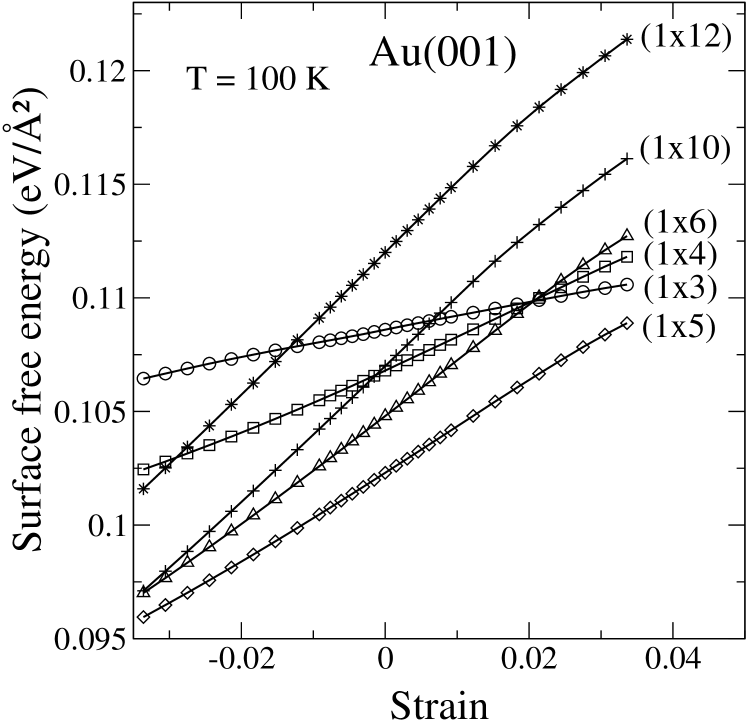
Figure 2: The free energy per unit area for some reconstructed Au(001) surfaces. In abscissa the strain at the surface due to bending is reported.

We continue our exemplification of the method to the (001) surface of gold, where we wish to calculate curvature-dependent free energies. We prepared different (001) slab samples, where the surfaces differ by a different reconstruction periodicity, in turn related to a different density of added atom rows perpendicular to the bending direction, that is parallel to the $x$-axis. In particular, in a $(1\times n)$ reconstruction one extra row is added every $n$ existing rows. After the usual equilibration steps the surfaces relax and equally spaced solitons appear, corresponding to misfit dislocations between first and second layer. The slabs are gradually bent and for each curvature the overall layer-resolved stress is computed through (4), the averages taken during a 36 $p$sec evolution time in a canonical simulation at $T=100K$. From the forces $T_{22}$ the surface contributions are extracted, as explained above. We plot the results in Fig. 2, where we have for convenience assumed arbitrarily the unknown zero-curvature free energy to be equal to the zero-temperature energy, calculated previously through MD by F. Ercolessi et al.[17]. At our working temperature of 100 K, this is likely a not unreasonable approximation.

All the surface free energies decrease with curvature on the concave side, where the compressive subsurface strain acts to reduce the need for a tensile surface stress. The decrease is more pronounced, as it should be, for the less dense higher reconstruction, whose tensile stress is higher. Although there are crossings, no other reconstruction crosses the $(1\times 5)$ surface free energy, which is therefore predicted to be stable against curvatures leading to surface strains up to the percent range.

Preliminary as these results are, they seem encouraging, although we do not yet have an alternative route to check them. It will be interesting in the future to carry out tests aimed among other things at separating the internal energy from the entropy part.

In conclusion, we have presented a calculation of surface free energy variation with curvature, realized by direct integration of surface stress, obtained through realistic molecular dynamics simulation. A specific application to (001) reconstructed gold surfaces shows a good feasibility of the method, and foreshadows future applications to study surface phase transitions under curvature.

Acknowledgments

We acknowledge support from MURST COFIN99, and from INFM/F. Research of D. P. in Stuttgart is supported by the Alexander Von Humboldt foundation.

References

- [1] L. D. Landau and E. M. Lifshitz, Statistical Physics, New York: Pergamon Press, 1980, chap. XV
- [2] H. Ibach, Surf. Sci. Rep. 29, 193 (1997)
- [3] M. W. Ribarsky and Uzi Landman, Phys. Rev. B 38, 9522 (1988)
- [4] O. H. Nielsen and R. M. Martin, Phys. Rev. B 32, 3780 (1985)
- [5] D. Passerone, E. Tosatti, G. L. Chiarotti and F. Ercolessi, Phys. Rev. B 59, 7687 (1999)
- [6] R. Koch and R. Abermann, Thin Solid Films 129, 63 (1985)
- [7] L. Huang, P. Zeppenfeld and G. Comsa, to be published and private communication
- [8] D. Frenkel, in Molecular Dynamics Simulations of Statistical Mechanics Systems, edited by G. Ciccotti and W. G. Hoover, Proceedings of the 97th Int. Enrico Fermi School of Physics, 1986
- [9] We observe that the curvature involves a non-uniform anisotropic strain, whence the system as a whole is out of equilibrium: thermodynamic arguments are only meaningful for the interface.
- [10] D. Passerone, U. Tartaglino, F. Ercolessi and E. Tosatti, accepted for publication in Surf. Sci.
- [11] H. C. Andersen, J. Chem. Phys. 72, 2384 (1980)
- [12] M. Parrinello and A. Rahman, J. Appl. Phys. 52, 7182 (1981)
- [13] F. Ercolessi, M. Parrinello and E. Tosatti, Phil. Mag. A 58, 213 (1988)
- [14] E. Tosatti and F. Ercolessi, Int. J. Mod. Phys. B 5, 413 (1991).
- [15] K. Yamazaki, K. Takayanagi, Y. Tanishiro and K. Yagi, Surf. Science 199, 595 (1988) and references therein.
- [16] C. E. Bach, M. Giesen and H. Ibach, Phys. Rev. Lett. 78, 4225 (1997)
- [17] F. Ercolessi, E. Tosatti and M. Parrinello, Phys. Rev. Lett. 57, 719 (1986); Surf. Science 177, 314 (1986)