Dirac quasiparticles in the mixed state
Abstract
Energies and wave functions are calculated for -wave quasiparticles in the mixed state using the formalism of Franz and Tes̆anović for the low-lying energy levels. The accuracy of the plane-wave expansion is explored by comparing approximate to exact results for a simplified one-dimensional problem, and the convergence of the plane wave expansion to the two-dimensional case is studied. The results are used to calculate the low-energy tunneling density of states and the low-temperature specific heat, and these theoretical results are compared to semiclassical treatments and to the available data. Implications for the muon spin resonance measurements of vortex core size are also discussed.
I Introduction
The nature of the low-lying excitations in the mixed state of a -wave superconductor is both an interesting quantum mechanics problem and important for understanding the behavior of high temperature superconductors in a magnetic field[1, 2, 3, 4, 5]. Volovik[1] first studied this problem in the semiclassical limit, where the -wave quasiparticles are Doppler shifted by the local superfluid density. The shifting of quasiparticle energies results in a non-zero density of states at zero energy proportional to the square root of the magnetic field. Volovik’s solution has been applied to calculations of the specific heat[6, 7, 8] thermal conductivity[9, 10], and nuclear magnetic relaxation rates[11, 12]. It has motivated useful discussions of the scaling behavior of the specific heat by Simon and Lee[13], Kopnin and Volovik[14], and others.
The presence of a magnetic field and its associated vortex lattice affects the motion of quasiparticles in four distinct ways. First, the quasiparticles, which carry current, move in the magnetic field which is approximately uniform for an extreme type-II superconductor. Second, although the field is approximately uniform, it is not exactly so, and therefore the quasiparticles experience magnetic field gradients. However the direct effect of these gradients is rather small. Third, there are supercurrents associated with the curl of the field, and the quasiparticle energies are affected by the corresponding superfluid velocity through which they move. For a uniform superfluid velocity field, the effect would be a simple Doppler shift of the energies. However, for inhomogeneous superfluid velocities the problem is more complicated. Fourth and finally, the magnitude of the superconducting order parameter is inhomogeneous in the mixed state, although this is mainly apparent within a coherence length of each vortex core where this magnitude falls to zero. For an extreme type-II superconductor, this represents a very small fraction of the sample for fields well below .
Volovik’s approach neglects the magnetic field and its gradients as well as the inhomogeneous order parameter amplitude and focuses only on the local supercurrent velocity. It assumes that the quasiparticle wave function can be thought of as a wave packet which is localized in a region over which the magnitude and direction of the superfluid velocity are relatively uniform. The energy of a low-lying, -wave quasiparticle depends linearly on , where is the wave vector of the nearest node. If a quasiparticle is localized in a region of size smaller than , then the spread in its energy will be larger than its average energy and the wavepacket picture does not work. For the superfluid velocity to be relatively uniform in a region, the size of the region must be smaller than the distance to the nearest vortex core and certainly smaller than, , the distance between vortices. Let us apply the above considerations to the lowest energy quasiparticle band. This corresponds to a quasiparticle, near node , with wave vector perpendicular to localized in a region of size . For the wavepacket picture to apply, the energy, , of the quasiparticle must be greater than , where is the quasiparticle velocity along . However for the superfluid velocity to be uniform in the region of size it is necessary that . Combining these two conditions we obtain the requirement that . For energies less than this the wavepacket picture breaks down and a full quantum mechanical picture is needed. This energy range is readily accessible via specific heat measurements below K in fields of one to several Tesla. It is this energy region that is the main focus of this paper.
Recently, Franz and Tes̆anović[4] (FT) have derived a quantum mechanical theory of the mixed state of a -wave superconductor, which involves a singular gauge transformation that maps the original problem of superconducting quasiparticles in a magnetic field onto an equivalent one of quasiparticles in a periodic potential. The latter problem may be solved using conventional band-structure methods.
In this paper, we investigate the low-energy properties of a -wave superconductor in the mixed state using the theory derived by Franz and Tes̆anović[4]. The most direct experimental probes of these properties are the low-energy tunneling density of states and the low temperature specific heat. In order to calculate these quantities reliably, we have investigated the numerical problem of Dirac quasiparticles in the periodic potential of the vortex lattice, focusing on the simplifications that result from the fact that the anisotropy of the Dirac cones, . As discussed by Mel’nikov[15], such large anisotropy makes the problem approximately one-dimensional. Mel’nikov described how to obtain solutions to the one-dimensional problem, but he then confined his analysis to the semiclassical versions of these solutions. We have explicitly evaluated the quantum mechanical solutions in this one-dimensional limit and used them as a test of the accuracy of approximate plane-wave solutions. We then show how to improve on the one-dimensional solutions by including a small number of plane wave basis states for the transverse direction, and we study the convergence of this approach.
The remainder of this paper is organized as follows. Section II addresses the computational problem of calculating quasiparticle energies in the lowest bands in the magnetic Brillouin zone, comparing exact and plane-wave-expansion solutions for the simplified one-dimensional problem and then comparing 1-D and 2-D plane-wave expansion solutions for various choices of plane-waves. Section III presents results for the local tunneling density of states, Sec. IV re-interprets recent muon spin resonance measurements of the vortex core size in terms of a scaling picture, and Sec. V presents calculations of the low temperature specific heat, comparing them to predictions based on Volovik’s approach and to experimental data.
II The Computational Problem: calculating the energies in the lowest bands in the magnetic Brillouin zone
The quasiparticle wavefunctions are described by the BdG equations, where , and
| (1) |
with . The gauge invariant form of the gap operator, , for a -wave superconductor can be written as (see Ref. [16] for the details)
| (2) |
where, for notational convenience, we have chosen to orient our axes along the directions of the gap nodes, at an angle of with respect to the orientation of the CuO2 planes. is the Fermi momentum, and is the Ginzburg-Landau order parameter. Since we are working in the intermediate field regime () of an extreme type II superconductor, we can assume that the magnitude of the gap is constant everywhere, except at the vortex cores, and that the magnetic field distribution and local superfluid velocity can be described by the London model[17].
In order to diagonalize the Hamiltonian in Eq. (1) one would like to remove the order parameter phase from the off-diagonal components of . It is desirable to choose a transformation which is both single-valued and treats the particles and holes on an equal footing. This is accomplished by the bipartite, singular gauge transformation of FT:[4]
| (3) |
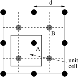
where , and and are the contributions to the order parameter phase from the and sublattices of the vortex lattice. The sublattices are chosen so that there are equal numbers of and vortices, with two vortices per magnetic unit cell of the vortex lattice. The vortex lattice configuration analyzed in this paper is shown in Fig. 1. Note that the fact that the - and -axes of the and sublattice unit cells are oriented along nodal directions means that nearest-neighbor lines of vortices are oriented along the - and -axes of the underlying crystal lattice.
Under this transformation becomes
| (4) |
where
| (5) |
with the superfluid velocities
| (6) |
Note that . Since the vortex lattice is periodic, the superfluid velocities can be written as Fourier sums
| (7) |
where , is the size of the magnetic unit cell, and is the displacement of or vortices from the center of the unit cell (see Fig. 1).
Linearizing the Hamiltonian in Eq. (4) at the node we find that with
| (8) |
and
| (9) |
where is the Fermi velocity, and is the slope of the gap at the node.
At the node the free Dirac Hamiltonian has the familiar Dirac cone spectrum
| (10) |
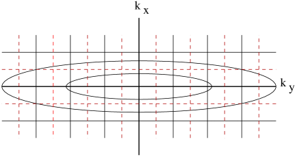
where at the node. The quasiparticle momentum along the nodal direction is with a corresponding wavelength of . If the energy is low enough (), will be confined to the first magnetic Brillouin zone (see Fig. 2) and the wavelength will exceed the intervortex distance , crossing the boundaries of several unit cells of the vortex lattice. For large values of the anisotropy the momentum parallel to the Fermi surface will be much larger than that along the nodal direction. The quasiparticle wavefunction will thus be localized in the direction parallel to the Fermi surface, but will be extended and will feel the average effect of the superfluid velocity fields of several vortices along the nodal direction.
Since the potential is periodic we can expand the quasiparticle wavefunction in the plane-wave basis:
| (11) |
The periodic potential of the vortex lattice will be responsible for the interaction of the Fourier components and . If we are interested only in energies below a cutoff energy, , for which the momentum lies well within the first MBZ we can make the approximation that the quasiparticle wavefunction is one-dimensional and ignore the interaction of those Fourier components that are at different values of . We therefore write
| (12) |
If, however, is high enough that exceeds the boundaries of the first MBZ (see Fig. 2) we can make the assumption–since the Fourier sum is dominated by components whose values of are bounded by the constant energy contour at –that
| (13) |
where is the cutoff wave vector along the y direction.
Such plane-wave expansions can be computed numerically to obtain the excitation spectrum for the quasiparticles in a periodic vortex lattice. The solution to the problem using Eq. (11) has been studied in detail by FT[4], whereas Marinelli, Halperin and Simon (MHS) [18] studied solutions to defined in Eqs. (8) and (9) in position space. Both groups found that the convergence of the plane-wave expansions was slow. Since we are specifically interested in the low energy and low temperature properties which are largely determined by the lowest band of the excitation spectrum, we will focus next on obtaining an analytical solution to the linearized Hamiltonian with the approximation that, for large , the quasiparticle wavefunctions are approximately one-dimensional. Having obtained both analytical and numerical solutions to this one-dimensional problem, we will then examine how adding more transverse wave vectors , as in Eq. (13), allows us to approach the exact numerical two-dimensional result, using Eq. (11).
A The 1-D analytical solution
At low energies and for large values of the wavefunctions are localized in the y direction and extended along the x direction.[15] This suggests the following basis as a useful starting point:
| (14) |
As we shall see, the Fourier components , for different , are spatially well separated in the y direction. Their interaction is consequently negligible, and we can assume that the Hamiltonian is diagonal in the quantum number . This allows us to replace the periodic potential in Eq. (9), which in principle scatters quasiparticles between states with different values of , with its effective potential averaged in the x direction which is diagonal in . The result is
| (15) |
where , where , , and where . Note that in these units , where . The potential along the y direction consists of two periodic sawtooth functions with discontinuities lying along the averaged vortex lines of the and sublattices. At sufficiently low energies the quasiparticles will be bound in the y direction by the potential barriers which lie at the discontinuities in . Our picture is thus one of quasiparticles that travel as plane-waves along the nodal direction but are bound within potential wells–created by the averaged vortex lattice–in the direction parallel to the Fermi surface. Note that, at low energies, the Fourier components and have negligible overlap, as they lie in separate potential wells along the y direction.
By making the substitution
Eq. 15 can be rewritten as
| (16) |
where and are the Pauli matrices. The function
is a sawtooth with a slope of and a period of , and the function
is a step function which oscillates between and with a period of . Since the potential is periodic we can solve Eq. (16) within a unit cell and use Bloch’s theorem to extend the solution over all of . The solution within a unit cell (see Appendix A for the details) is given in terms of the parabolic cylinder functions :[19]
| (17) |
for and
| (18) |
for , with and .
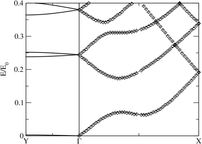
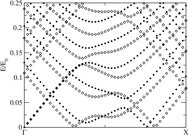
These solutions can be matched at the boundaries of the unit cell (see Appendix B) to obtain an exact excitation spectrum for the one-dimensional, averaged Hamiltonian. The resulting spectrum for anisotropy is shown in Fig. 3. It is useful to note that the energy scale is approximately given by .
B Comparison of 1-D analytical and plane-wave expansion results
Using the plane-wave expansion of Eq. (12) we can numerically diagonalize the Hamiltonian to obtain an excitation spectrum that can be compared with the analytical results. To the numerical accuracy of the diagonalization, these two methods yield identical results for the dispersion along as shown in Fig. 3, where 61 reciprocal lattice vectors (RLVs) have been kept in the plane-wave expansion.[20] The dispersion along calculated from the 1-D plane-wave expansion is also shown in Fig. 3. As discussed by MHS, [18] the dispersion away from the point along is more strongly renormalized by the supercurrents, leading to an enhanced effective . For there is essentially no discernable dispersion along for the lowest bands (as calculated in either the 1-D or full 2-D plane-wave expansions), further suggesting the validity of a one-dimensional approximation.
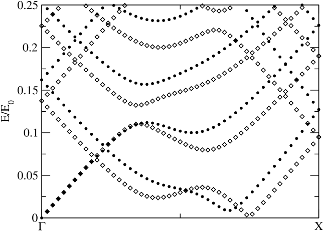
Since both the energy and momentum axes scale as these spectra apply to all values of the magnetic field within . As the anisotropy increases, the gap between the lowest band of the spectrum and the axis quickly narrows. At (Fig. 4) the spectrum is close to forming a line quasinode, in agreement with the results of FT[4], and of MHS [18], which suggest that a line quasinode first appears at .
C Comparison of 1-D and approximate 2-D plane-wave calculations
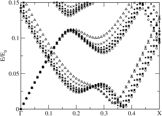
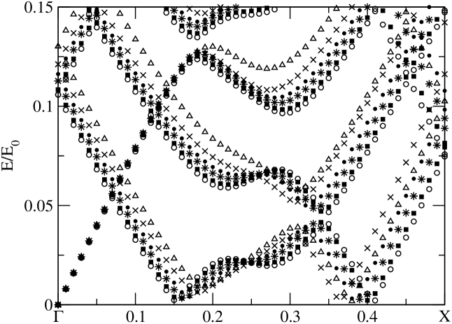
The results of numerical diagonalization calculations of the excitation spectrum of the quasiparticles in the 1-D averaged potential and the exact 2-D potential at different values of the anisotropy are shown in Figs. 4 and 5. The 1-D spectra show good qualitative agreement with the 2-D spectra, capturing the major features of the lowest bands, including the line quasinodes that form at large values of . However, the 1-D treatment is unable to accurately represent, quantitatively, the behavior of the full 2-D spectrum. In particular, as can be seen from Figs. 4 and 5, the 1-D approximation cannot be used to quantitatively determine the size of the minigaps which lie along the line quasinodes. An analysis of the 1-D spectra for several values of shows that the size of the smallest minigap at fixed is where . Unfortunately, the slow convergence of the 2-D reciprocal lattice sums–due to the divergence of the superfluid velocity at the vortex cores (discussed in more detail by Vafek et al.[16])–makes it very difficult to accurately determine the size of these minigaps in the full 2-D calculation.
Nonetheless, we believe that the 1-D treatment (which is far less computationally intensive than the 2-D problem) captures and elucidates the important physics of the lowest bands of the quasiparticle excitation spectrum and is therefore a useful tool that helps us understand the physical behavior of the quasiparticles in the mixed state. In particular we will use the 1-D energies and wave functions to calculate the local tunneling density of states and the specific heat.
Next we compare the results of the 1-D calculations to finite 2-D plane wave expansions using a grid of reciprocal lattice vectors. For example, in Fig. 6 results are shown for , comparing the 1-D case, , to 5, 9, 13, 21, and 29, . Similar results are shown in Fig. 7 for and . One of the most striking features of both figures is the complete insensitivity of the linear branch near the point to the number of plane-waves in the calculation. For this branch, it appears that the 1-D energies are essentially exact. For other low-energy branches and general points in the Brillouin zone, the plane-wave expansion seems to converge smoothly. The only pathological behavior occurs near the quasinodes, where both the positions and the values of the minima converge slowly.
III Local Tunneling Density Of States
In this section we show results of calculations of the local tunneling density of states (TDOS) of the quasiparticles in the lowest band of the energy spectrum using the one-dimensional plane-wave expansion of Eq. (12). The TDOS is:[21, 22]
| (19) | |||||
| (20) |
where is the derivative of the Fermi function, is the set of wave vectors in the magnetic Brillouin zone, is the set of energy bands (restricted in this case to the lowest positive and negative energy bands) and is the set of four Dirac nodes. The normalization factor is equal to the number of spins divided by the number of wave vectors in the magnetic Brillouin zone. The extra factor of 2 is an artifact of the normalization in the diagonalization routine used.
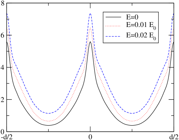
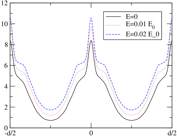
The plane-wave expansion was done at the node . It is easy to show that by taking in Eq. (19) one obtains the contribution from the opposite node at . Within the 1-D approximation, these two nodes give the y dependence of the TDOS, and the other two nodes at give the x dependence. The y (or x) dependence of the TDOS at 1 Kelvin and at a field of 1 Tesla, for two different values of the anisotropy , and at three different energies is shown in Figs. 8 and 9.
One can see that the TDOS has the periodicity of, and is sharply peaked at, the vortex lines. The TDOS falls to a broad minimum in the regions between the vortices. The shoulders on either side of the peaks come from the states within the lines of quasinodes that form at large values of . At , the size of the gap in the line quasinode has decreased and a second line quasinode has started to appear (see Fig. 5). Both these features contribute to the very distinct shoulders on either side of the peak in the TDOS in Fig. 9.
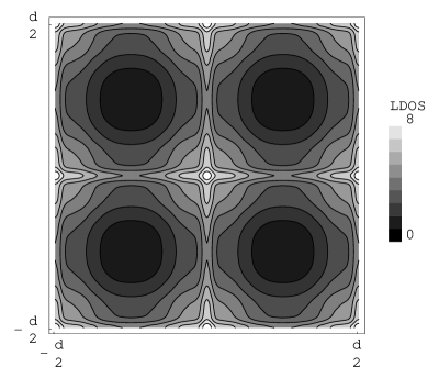
Figure 10 shows the zero-bias two-dimensional TDOS as a sum over the four nodes. This result is in qualitative agreement with the semiclassical calculation of the TDOS by Mel’nikov [23]. The vortex lattice geometry of our paper is, in Mel’nikov’s notation, a Type II lattice with . This gives a TDOS that is proportional to
| (21) |
where . The semiclassical TDOS of Mel’nikov thus has the profile of a triangle wave along the x and y directions. The fully quantum mechanical results shown here follow this profile, but exhibit additional structure that arises from the quasiparticle states near the quasinodes.
We note that only half of the bright spots in Fig. 10 lies at vortex positions while the other half lies halfway between vortices. For example, in Fig. 10 the bright spots at the corners and at the center of the figure might correspond to vortex sites. The other bright spots are then the result of the overlap of the sharply peaked tunneling density of states which extends from each vortex, parallel to the four node directions. It is an artifact of the 1-D model that, for the case of a square lattice, these overlaps have a peak tunneling density of states equal to that of a vortex core. This artifact is less evident in more general, centered rectangular lattices or, in particular, for the hexagonal lattice.[15, 23]
IV Muon Spin Resonance
Two important simplifying assumptions in this model are that the superconducting coherence length is negligible and that the penetration depth is large compared to the distance between vortices. As a consequence of these assumptions, the intervortex spacing is the only length scale in the problem. This allows us to present results scaled to this length as is done above for the tunneling density of states.
In addition to the tunneling density of states, one could also use the wave functions generated by these calculations to compute the pattern of the two-dimensional supercurrent density. This would, of course, not be a self-consistent result, but it would be an improvement over the initial form for the supercurrent density corresponding to Eq. (7). Without actually doing this calculation, we know that the resulting pattern would be a function of and hence that all lengths would scale as .
This picture, in which the vortex lattice constant provides the only length scale, is supported by the self-consistent calculations of Franz and Tesanovic for a single -wave vortex. [24] In Fig. 1 of Ref. [24] and the accompanying discussion, it is shown that, for systems with very short coherence lengths, the spatial dependence of the gap function outside the core has a scale-independent power-law dependence, approaching its asymptotic value roughly as .
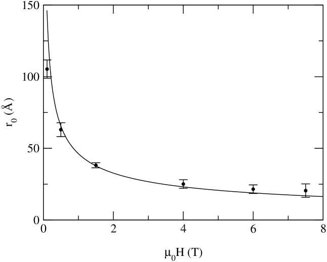
The above discussion provides a natural explanation of the muon spin resonance results of Sonier and co-workers[25] who found that the vortex core radius, defined as the radius at which the supercurrent density has its maximum, grows large at low field. In fact, an excellent fit to their data can be obtained by assuming that the vortex core radius scales as , as is shown in Fig. 11. The coefficient of from the fit is . Since the vortex lattice constant for the or sublattices is , this maximum occurs at about 7% of or equivalently at about 10% of the intervortex spacing. It would be interesting to test this result at higher fields to see if this scaling breaks down and if saturates at a constant value limited by the coherence length as one might expect.
V The Density of States and the Specific heat
A Semiclassical DOS
We start by calculating the density of states for the semiclassical (SC) approximation, in which the energy is Doppler shifted by the local superfluid velocity :
| (22) |
where the spectrum has been linearized around the node .
The local superfluid velocity far from the vortex is . In the commonly employed “single-vortex approximation,” the associated density of states is
| (24) | |||||
where the factor of accounts for spin degeneracy. is the total area of the CuO planes in the sample, where is the volume of the sample and is the average separation between the planes, and is the area of one unit cell of the vortex lattice. The integral is over .
In the absence of a magnetic field, with no Doppler shift,
| (25) |
Putting the magnetic field back in, the density of states has the intercept
| (26) |
where is the zero-field density of states. For nonzero we find that
| (27) |
for , where , and
| (28) |
for . Note that this is the contribution to the total density of states for 2 spin states from one of the four nodes.
A more realistic calculation of the semiclassical DOS can be made for a square vortex lattice if we write the superfluid velocity as the Fourier sum
| (29) |
where and . Note that we are now orienting the x and y axes along the nearest-neighbor directions of the square vortex lattice. The corresponding density of states,
| (30) |
can then be calculated numerically using this more accurate expression for . The semiclassical density of states, as calculated for both the single-vortex approximation and the square vortex lattice, is shown in Figs. 12 and 13. One can see that the square-lattice DOS is about 30% lower at zero energy than that calculated using the single-vortex approximation. This lowering is caused by the disappearance of at high symmetry points on the vortex-lattice unit-cell boundary.[26]
B Quantum DOS
The quantum density of states is calculated from the quasiparticle energy spectrum at the node :
| (31) |
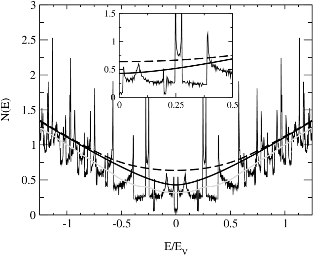
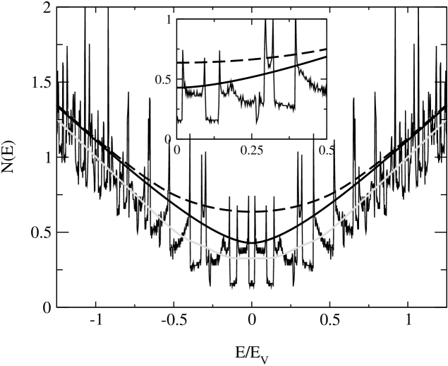
where n labels the energy bands and is a wave vector in the magnetic Brillouin zone. The factor of accounts for spin degeneracy. In order to clarify the dimensional analysis, we have multiplied the usual expression by , where is the number of wave vectors in the MBZ, and is the total area of the CuO planes in the sample. The energy in this expression is in units of . In order to compare this result with the semiclassical result we simply write in units of [see Eq. 25], noting that . Results are shown in Figs. 12 and 13, where comparison is made to both the SC single-vortex approximation and to the SC square-lattice DOS. Note that both axes scale as . The dotted line shows the commonly employed single vortex SC DOS to be roughly twice as large as the quantum 1-D DOS in the low-energy region. The quantum DOS rises more quickly with energy and the SC and quantum DOS match up at higher energy andare indistinquishable for energies above 3. The discrepancy between the SC square-lattice calculation and the quantum DOS at low energies is due to quantum effects that average over the rapid variations in the direction of near the vortex cores as well as near the high symmetry points on the unit-cell boundary. Of course, disorder effects on the vortex lattice and the quasiparticle energies will also affect the average magnitude of the low-energy DOS in both the SC and quantum cases.[8, 26]
The 1-D calculation of for (Fig. 13) is in good agreement with the corresponding 2-D calculation of FT[4], reproducing all of the major features at low energies. The overall magnitude of the 1-D DOS is slightly reduced from the full 2-D calculation. The 1-D calculation, by essentially averaging in one direction, underestimates the effect of the supercurrents, which push states to lower energies, as can be seen from the bandstructures shown in Figs. 4 and 5. The full 2-D quantum DOS in Ref. [4], is about 10% higher in magnitude than the 1-D approximation, but is still noticeably lower in magnitude than the SC square-vortex-lattice result.
C Scaled
The heat capacity of a fermion gas is
| (32) | |||||
| (33) |
This is the expression used to calculate the specific heat () from the total density of states . The total density of states in Eq. (33) is a sum over the density of states for one spin at each of the four nodes. Thus, where is the semiclassical [Eqs. 27 & 28] or quantum mechanical [Eq. 31] density of states calculated in the previous section. Therefore, the specific heat at constant volume is
| (34) |
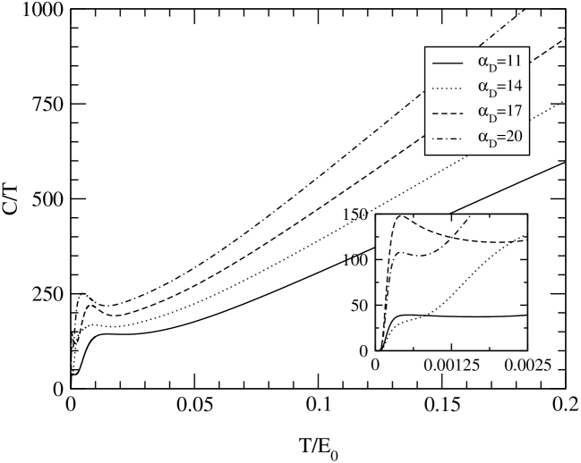
The specific heat for the 1-D calculation is shown for various values of in Fig. 14. Again, both the axis and the axis scale as , in agreement with the general scaling predictions of Volovik[1], and Simon and Lee[13]. The is linear at higher temperatures, flattens out as the temperature is decreased, and then increases to a peak at even lower before rapidly falling, with a tiny shoulder on the way down (see inset of Fig. 14), to zero at . The large peak both sharpens and moves closer to the axis as the anisotropy is increased. The behavior of this peak suggests that its presence is due to the low energy peaks in the DOS, particularly the van Hove singularities that occur just above for as these contribute significant weight to the DOS. A narrow peak at in the DOS will typically show up as a peak in the specific heat near .[29] Comparing the 1-D and 2-D dispersions and DOS, we expect this peak to shift to slightly lower energy and to sharpen in the full 2-D calculation of the specific heat.
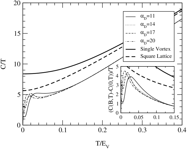
The SC specific heat, for the square lattice and for the single-vortex approximation, is shown in Fig. 15, along with the 1-D specific heat. The temperature is in units of and is in units of
| (35) |
Again, the main difference between the SC and quantum specific heat is that the SC specific heat larger in magnitude. Both exhibit the same scaling with magnetic field and with . The quantum specific heat exhibits structure at the lowest temperatures which is a reflection of the structure in the low-energy DOS.
In order to make comparisons with experimental results, we use the numbers in Chiao et al.[27] for YBCO: , , and Å. The molar volume of YBCO is .[28] With these numbers we obtain an intercept for the SC single vortex calculation of in seemingly excellent agreement with the experimental coefficient of of Moler et al.[6]. However, since this approximation overestimates the zero energy specific heat by roughly a factor of 2, this agreement is fortuitous. The quantum specific heat for flattens out at approximately .
The Geneva group of Junod and co-workers has reported a number of results[7, 30] for the specific heat of very high quality YBCO crystals, grown in crucibles and doped to so as to minimize the effects of oxygen chain vacancies. In the earlier of these, Revaz et al.,[7] the vortex contribution to the specific heat was obtained by subtracting from , the idea being that both lattice and magnetic impurity effects would cancel out in this subtraction and that the vortex contribution to the spceific heat for is small. In the more recent preprint by Wang et al.[30], results are presented for for . For our purposes, these data are more directly useful since they involve only the single field direction that we have studied. Furthermore, the results should be reliable, since the samples show very little sign of point magnetic impurities. Wang et al.[30] find a intercept for of (mJ mol-1)K-2T-1/2.
In order to compare our theoretical results to the and dependence found by Wang et al.,[30] we need to subtract the specific heat in zero field from that in a field. The result is shown in the inset of Fig. 15. It is interesting that the structure that we find at the lowest temperatures could easily be attributed to Schottky-type anomalies in the data. In fact Wang et al. [30] show figures with and without subtraction of an assumed Schottky anomoly, and the latter better resembles our theoretical results. It is tempting to suggest that the experimentally observed low temperature structure in samples with the least magnetic impurities is actually due to the structure in the quasiparticle density of states. However, since the magnitude of the observed field-dependent specific heat is more than twice as large as the calculated value, such detailed comparisons between theory and experiment are probably premature. The effect of disorder on the quasiparticles would likely increase the low energy specific heat, since it increases the low energy DOS. On the other hand, disorder in the vortex lattice may equally well decrease the low-energy specific heat by reducing the local supercurrent velocity. Therefore, it is not obvious that disorder, in itself, can account for the differences between theory and experiment.
VI Conclusions
By making the approximation, in the mixed state, that the low-energy quasiparticle states in the Dirac nodes are essentially one-dimensional, we have been able to obtain analytical results for the quasiparticle wave functions and energy spectra. The 1-D approximation to the FT Hamiltonian[4] elucidates the physics of the interaction of the quasiparticles in the lowest-energy bands with the vortex lattice: the quasiparticles travel as plane-waves along the directions of the gap nodes, and are confined by the periodic potential of the vortex lattice in the direction of the Fermi surface. Using these exact analytical results, we were able to show that the approximate plane-wave solution for the same problem converges rapidly. The 1-D approximation is able to reproduce the important features of the 2-D plane-wave expansion in the lowest bands.
We have presented calculations of the tunneling density of states, which are in qualitative agreement with the semiclassical results of Mel’nikov[23] but which also show spatial structure due to the energy dispersion of the low-lying states. The density of states at zero energy for the quantum problem is significantly lower (by a factor of 2) than the commonly-employed semiclassical result for a single circular vortex, although this simple approximation overestimates the semiclassical density of states for a square vortex lattice configuration by roughly 30% at zero energy. Thus this reduction arises from two sources: the larger area of low superfluid velocity in the Abrikosov lattice, compared to the case of a single vortex in a circular unit cell of radius , and quantum averaging of the superfluid velocity for quasiparticles in the first magnetic Brillouin zone.
The specific heat has been calculated from the DOS of the 1-D plane-wave expansion and found to exhibit structure at low temperatures that is not present in the semiclassical approximation. In addition, the magnitude of the low- temperature specific heat is reduced by quantum effects. Since the values of the specific heat measured experimentally,[6, 7, 30] for parameters and taken from other experiments, are already larger than the semiclassical results, the disagreement in magnitude with the quantum results are even larger. One possibility is that the discrepancy is due to the effects of disorder which, to date, have not been included in any quantum treatment of the specific heat. Other possibilities are that the parameters are such that is substantially larger than is currently believed, or that there are additional low-energy states not accounted for in the disordered -wave model but which exhibit similar magnetic-field dependence.
ACKNOWLEDGMENTS
We would like to thank Marcel Franz, Peter Hirschfeld, Elisabeth Nicol, Zlatko Tesanovic, Ilya Vekhter and Rachel Wortis for useful discussions and correspondence and Jeff Sonier for discussing and sharing his MuSR results with us. We thank the Institute for Theoretical Physics, where this work was completed, for their hospitality. This research was supported in part by the Natural Sciences and Engineering Research Council (Canada) and by the National Science Foundation under Grant No. PHY94-07194.
A Analytical solution of the 1-D problem
With the approximation that the potential is one-dimensional the quasiparticle Hamiltonian is
| (A1) |
The Hamiltonian can be rewritten as
| (A2) |
where , and . Borrowing a trick from Mel’nikov [15], one can insert between and and then multiply Eq. (A2) on the left by . This transformation takes and vice versa. We then write
so that
| (A3) | |||
| (A4) |
where . Writing we obtain the following coupled first-order differential equations:
From these coupled equations we can derive a second order differential equation for :
| (A5) | |||||
| (A6) | |||||
| (A7) |
with delta functions at the boundaries and at the center of the unit cell. In the regions and , the second order differential equation for is
| (A8) | |||||
| (A9) |
Since this differential equation is periodic in , we can solve it within a unit cell and use Bloch’s theorem to extend the solution over all of . Since has a period of and has a period of , we divide the unit cell into two regions (taking for simplicity): and . In these two regions
and
Taking region 1 as and region 2 as we can write
| (A10) |
where and , , and . If we let then
| (A11) |
This equation is solved by the parabolic cylinder functions (see Gradshteyn and Ryzhik [19])
| (A12) |
where . The corresponding solution for is easily obtained. We thus obtain the full solution for shown in Eqs. (17) and (18).
B Solution of the boundary conditions to obtain an excitation spectrum
Acceptable solutions must be continuous at the interior point, , and at the boundaries of the unit cell, . At the boundary condition is
which can be rewritten as
| (B5) |
At the boundary condition is
or
| (B8) |
where we have used the periodicity of on the right hand side of the above equation. From Eqs. (B5) and (B8) we can write
| (B9) |
where
| (B10) |
Since the Hamiltonian is periodic the eigenvalues of , an operator which induces a translation of one period, must satisfy the Bloch condition:
| (B11) |
where . The eigenvalues of are the roots of the characteristic equation
| (B12) |
Clearly
| (B13) |
which implies that
| (B14) |
Since is real
| (B15) |
and
| (B16) |
The energy spectrum can now be directly calculated using this expression.
REFERENCES
- [1] G. E. Volovik, JETP Lett. 58, 469 (1993).
- [2] L. P. Gor’kov and J. R. Schrieffer, Phys. Rev. Lett. 80, 3360 (1998).
- [3] P.W. Anderson, cond-mat/9812063.
- [4] M. Franz and Z. Tes̆anović, Phys. Rev. Lett. 84, 554 (2000).
- [5] B. Jankó, Phys. Rev. Lett. 82, 4703 (1999).
- [6] K. A. Moler, D. L. Sisson, J. S. Urbach, M. R. Beasley, A. Kapitulnik, D. J. Baar, R. Liang and W. N. Hardy, Phys. Rev. B 55, 3954 (1997).
- [7] B. Revaz, J. Y. Genoud, A. Junod, K. Neumaier, A. Erb, and E. Walker, Phys. Rev. Lett. 80, 3364 (1998).
- [8] C. Kubert and P.J. Hirschfeld, Sol. St. Comm. 105, 459 (1998).
- [9] J. Franz, Phys. Rev. Lett. 82, 1760 (1999).
- [10] C. Kubert and P.J. Hirschfeld, Phys. Rev. Lett. 80, 4963 (1998).
- [11] R. Wortis, A. J. Berlinsky, and C. Kallin, Phys. Rev. B 61, 12342 (2000).
- [12] D. K. Morr and R. Wortis, Phys. Rev. B 61, R882 (2000).
- [13] S. H. Simon and P. A. Lee, Phys. Rev. Lett. 78, 1548 (1997).
- [14] N. B. Kopnin and G. E. Volovik, JETP Lett. 64, 690 (1996).
- [15] A. S. Mel’nikov, J. Phys. Condens. Matter 11, 4219 (1999).
- [16] O. Vafek, A. Melikyan, M. Franz, and Z. Tes̆anović, cond-mat/0007296 v2.
- [17] F. and H. London, Proc. Roy. Soc. London, Sr. A 149, 71 (1935).
- [18] L. Marinelli, B. I. Halperin and S. H. Simon, cond-mat/0001406.
- [19] I. S. Gradshteyn and I. M. Ryzhik, Table of Integrals, Series and Products. Academic Press: New York (1980).
- [20] In the 1-D plane-wave expansions, convergence is achieved by keeping 41 RLVs for and 61 RLVs for .
- [21] F. Gygi and M. Schluter, Phys. Rev. B 41, 822 (1990).
- [22] Y. Wang and A. H. MacDonald, Phys. Rev. B 52, R3876 (1995).
- [23] A. S. Mel’nikov, cond-mat/9912455.
- [24] M. Franz and Z. Tesanovic, Phys. Rev. Lett. 80, 4763 (1998).
- [25] J.E. Sonier et al. Phys. Rev. Lett. 83, 4156 (1999).
- [26] I. Vekhter, P.J. Hirschfeld and E.J. Nicol, cond-mat/0011091.
- [27] M. Chiao, R. Hill, C. Lupien, L. Taillefer, P. Lamber, R. Gagnon, and P. Fournier, Phys. Rev. B 62, 3554 (2000).
- [28] A. Simon, J. Solid State Chem. 77, 200 (1998).
- [29] See, for example, the discussion on Schottky anomalies in C. Kittel, Thermal Physics, John Wiley & Sons, New York, 1969.
- [30] Y. Wang et al., cond-mat/0009194.