Magnetization Plateau of an $S=1$ Frustrated Spin Ladder

The magnetization plateaux of low dimensional spin systems have been attracting much attention because of its full quantum nature. Very recently, a new organic tetraradical, 3,3’,5,5’-tetrakis(N-tert-butylaminoxyl)biphenyl, abbreviated as BIP-TENO, has been synthesized.${}^{\hbox{\immediate{\bf{?}})}}$ This material can be regarded as an $S=1$ antiferromagnetic two-leg spin ladder, as explained later. Goto et al.${}^{\hbox{\immediate{\bf{?}})}}$ measured the magnetization curve of BIP-TENO at low temperatures in pulsed high magnetic fields up to about 50 T. They found $M\simeq 0$ up to about $H_{\rm c1}\simeq 10\,{\rm T}$, suggesting the non-magnetic ground state, which was consistent with the result of susceptibility measurement. Another remarkable nature of their magnetization curve is the plateau at $M=M_{\rm s}/4$ above $H_{\rm c2}\simeq 45\,{\rm T}$, where $M_{\rm s}$ is the saturation magnetization. Unfortunately the end of the $M_{\rm s}/4$ plateau is unknown because of the limitation of the strength of their magnetic field.

Considering the structure of BIP-TENO, Katoh et al.${}^{\hbox{\immediate{?})}}$ proposed its model of Fig.1. Since the ferromagnetic coupling $J_{\rm F}$ is thought to be much larger than other antiferromagnetic couplings $J^{\prime}_{\rm AF}$ and $J_{\rm AF1}$, two spins coupled by $J_{\rm F}$ effectively form an $S=1$ spin. Thus the model of Fig.1(b) is reduced to an $S=1$ antiferromagnetic two-leg ladder, as shown in Fig.1(c). The relation between the coupling constants of these two models are

$$J_{\perp}=J_{\rm AF1},~{}~{}~{}~{}~{}J_{1}=(1/4)J^{\prime}_{\rm AF}.$$ (1)

In the following, we consider the model of Fig.1(c) to investigate the $M_{\rm s}/4$ magnetization plateau of this model at zero temperature.

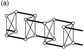
Fig.  1: (a) Schematic illustration of BIP-TENO. Open circles represent $S=1/2$ spins. (b) Plane type illustration of BIP-TENO. (c) Effective model of BIP-TENO in case of $J_{\rm F}\to\infty$. Open ellipses represent $S=1$ spins.

The plateau at $M=0$ is interpreted as the manifestation of the Haldane state. On the other hand, the $M_{\rm s}/4$ plateau is not easily understood. The necessary condition for the quantized magnetization plateau by Oshikawa, Yamanaka and Affleck${}^{\hbox{\immediate{\bf{?}})}}$ is

$$Q(S_{\rm unit}-\langle m\rangle)={\rm integer},$$ (2)

where $Q$ is the spatial period of the wave function of the state measured by the unit cell, $S_{\rm unit}$ and $\langle m\rangle$ are the total spin and the magnetization per unit cell, respectively. Applying the theorem to our model, $S_{\rm unit}=2$ and $m=1/2$, this condition is not satisfied if $Q=1$. Thus, $Q=2$ is required at least, which means the occurrence of the spontaneous symmetry breaking in the $M_{\rm s}/4$ plateau state. The magnetization plateaux caused by the spontaneous symmetry breaking were discussed for the $M_{\rm s}/2$ plateau of the $S=1/2$ zig-zag ladder${}^{\hbox{\immediate{\bf{?}},\penalty 1000\hskip 0.91003pt plus 0.70004pt minus 0.70004pt{\bf{?}},\penalty 1000\hskip 0.91003pt plus 0.70004pt minus 0.70004pt{\bf{?}})}}$ (equivalent to the bond-alternating chain with next-nearest-neighbor interactions), the $M_{\rm s}/2$ plateau of the $S=1/2$ ladder,${}^{\hbox{\immediate{\bf{?}},\penalty 1000\hskip 0.91003pt plus 0.70004pt minus 0.70004pt{\bf{?}},\penalty 1000\hskip 0.91003pt plus 0.70004pt minus 0.70004pt{\bf{?}},\penalty 1000\hskip 0.91003pt plus 0.70004pt minus 0.70004pt{\bf{?}})}}$ and also the $(2/3)M_{\rm s}$ plateau of the $S=1/2$ distorted diamond chain,${}^{\hbox{\immediate{\bf{?}},\penalty 1000\hskip 0.91003pt plus 0.70004pt minus 0.70004pt{\bf{?}})}}$ and so on.

The Hamiltonian of the model of Fig.1(c) is

$$\hat{H} = J_{1}\sum_{l=1,2}\sum_{j=1}^{L}{\mbox{\boldmath$S$}}_{l,j}\cdot{\mbox{\boldmath$S$}}_{l,j+1}+J_{\perp}\sum_{j=1}^{L}{\mbox{\boldmath$S$}}_{1,j}\cdot{\mbox{\boldmath$S$}}_{2,j}$$ (3)

$$~{}~{}~{}~{}~{}+H\sum_{l=1,2}\sum_{j=1}^{L}S^{z}_{l,j}$$

where $S$ denotes the spin-1 operator, $j$ the rung number and $l=1,2$ the leg number. The last term is the Zeeman energy in the magnetic field $H$. When $J_{\perp}=0$, our model is reduced to that of two independent usual $S=1$ chains, in which no plateau is expected in the magnetization curve except at $M=0$.

Let us consider the opposite limit $J_{\perp}\gg J_{1}$ by use of the degenerate perturbation theory. When $J_{1}=0$, all the rung spin pairs are mutually independent. In this case, at $M_{\rm s}/4$, half of the rung spin pairs are in the state

$$\psi(0,0)=(1/\sqrt{3})(|\uparrow\downarrow\rangle+|\downarrow\uparrow\rangle-|00\rangle)$$ (4)

and the remaining half pairs are in the state

$$\psi(1,1)=(1/\sqrt{2})(|\uparrow 0\rangle+|0\uparrow\rangle)$$ (5)

where $\psi(S_{\rm tot},S_{\rm tot}^{z})$ is the wave function of two $S=1$ spins coupled by antiferromagnetic interaction $J_{\perp}$ with the quantum numbers $S_{\rm tot}$ and $S_{\rm tot}^{z}$. These wave functions have lowest energies in the subspace of $S_{\rm tot}^{z}=0$ and $S_{\rm tot}^{z}=1$, respectively. Other possible selections have higher energies. The $M_{\rm s}/4$ state is highly degenerate as far as $J_{1}=0$, because there is no restriction for the configurations of these two states. This degeneracy is lifted up by the introduction of $J_{1}$. To investigate the effect of $J_{1}$, we introduce the pseudo-spin $T$ with $T=1/2$. The $|\Uparrow\rangle$ and $|\Downarrow\rangle$ states of the $T$ spin correspond to $\psi(1,1)$ and $\psi(0,0)$, respectively. Neglecting other seven states for the rung spin pairs, the effective Hamiltonian can be written as

$$\hat{H}_{\rm eff}=\sum_{j}\left\{J_{\rm eff}^{xy}(T_{j}^{x}T_{j+1}^{x}+T_{j}^{y}T_{j+1}^{y})+J_{\rm eff}^{z}T_{j}^{z}T_{j+1}^{z}\right\}$$ (6)

in the lowest order of $J_{1}$, where

$$J_{\rm eff}^{xy}=(8/3)J_{1},~{}~{}~{}~{}~{}J_{\rm eff}^{z}=(1/2)J_{1}$$ (7)

Thus the $M_{\rm s}/4$ plateau problem of the original model is mapped onto the $M=0$ problem of the usual $T=1/2$ antiferromagnetic $XXZ$ spin chain with the nearest-neighbor (NN) interaction. As is well known, depending on whether $\Delta_{\rm eff}\equiv J_{\rm eff}^{z}/J_{\rm eff}^{xy}\leq 1$ or $\Delta_{\rm eff}>1$, the ground state of eq.(6) is either the spin-fluid state (gapless) or the Néel state (gapful), which correspond to the no-plateau state or the plateau state of the original model, respectively.

We see $\Delta_{\rm eff}=3/16$ from eq.(7), which means no $M_{\rm s}/4$ plateau in the model of Fig.1(c), at least when $J_{\perp}\gg J_{1}$. As already stated, there is no $M_{\rm s}/4$ plateau also when $J_{\perp}=0$. Thus the $M_{\rm s}/4$ plateau will not appear in the whole region of $J_{1}/J_{\perp}$ for the model of Fig.1(c), although we cannot completely exclude the possibility of the $M_{\rm s}/4$ plateau at the intermediate region. We note that the absence of the $M_{\rm s}/4$ plateau is also established by numerical method, as shown later in Fig.4.

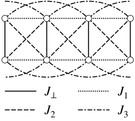
Fig.  2: $S=1$ ladder model with second and third neighbor interactions.

In previous works for the $M_{\rm s}$/2 plateau of the $S=1/2$ spin ladder,${}^{\hbox{\immediate{?},\penalty 1000\hskip 0.91003pt plus 0.70004pt minus 0.70004pt{?},\penalty 1000\hskip 0.91003pt plus 0.70004pt minus 0.70004pt{?},\penalty 1000\hskip 0.91003pt plus 0.70004pt minus 0.70004pt{?})}}$ it has shown that the second and/or third neighbor interactions bring about the plateau. Considering this fact, let us introduce the second ($J_{2}$) and third ($J_{3}$) neighbor interactions to our model, as shown in Fig.2. Including these interactions, the effective Hamiltonian (6) is modified to the generalized version of the $T=1/2$ $XXZ$ Hamiltonian with the NN and the next-nearest-neighbor (NNN) interactions:

$$\hat{H}_{\rm eff}=\sum_{j}\left\{J_{\rm eff}^{xy}(T_{j}^{x}T_{j+1}^{x}+T_{j}^{y}T_{j+1}^{y})+J_{\rm eff}^{z}T_{j}^{z}T_{j+1}^{z}\right\}$$

$$+\sum_{j}\left\{J_{\rm eff}^{xy(2)}(T_{j}^{x}T_{j+2}^{x}+T_{j}^{y}T_{j+2}^{y})+J_{\rm eff}^{z(2)}T_{j}^{z}T_{j+2}^{z}\right\}$$ (8)

where

$$J_{\rm eff}^{xy}=(8/3)(J_{1}-J_{2}),~{}~{}~{}~{}~{}J_{\rm eff}^{z}=(1/2)(J_{1}+J_{2})$$ (9)

$$J_{\rm eff}^{xy(2)}=(8/3)J_{3},~{}~{}~{}~{}~{}~{}~{}~{}~{}~{}~{}J_{\rm eff}^{z(2)}=(1/2)J_{4}$$ (10)

Note that the $XXZ$ anisotropy parameters of the NN and NNN interactions are different with each other in general. In this model, three phases are expected:${}^{\hbox{\immediate{\bf{?}},\penalty 1000\hskip 0.91003pt plus 0.70004pt minus 0.70004pt{\bf{?}})}}$ these are the spin-fluid state (gapless), the Néel state (gapful) and the dimer state (gapful).

For simplicity, first we consider the $J_{2}>0,J_{3}=0$ case. In this case, the NNN interaction in eq.(8) vanishes and the anisotropy parameter is

$$\Delta_{\rm eff}={3\over 16}\,{J_{1}+J_{2}\over J_{1}-J_{2}}$$ (11)

Therefore the Néel condition $\Delta_{\rm eff}>1$ is satisfied when $J_{2}/J_{1}>13/19$. This type of $M_{\rm s}/4$ plateau is due to the Néel mechanism and called plateau A from now on.

Next we consider the $J_{2}=0,J_{3}>0$ case. In this case, the anisotropy parameters of the NN and NNN interactions have the same value $\Delta_{\rm eff}=3/16$ and $J_{\rm eff}^{xy(2)}/J_{\rm eff}^{xy}=J_{\rm eff}^{z(2)}/J_{\rm eff}^{z}=J_{3}/J_{1}$. From the phase diagram of $S=1/2$ $XXZ$ chain with the NN and NNN interactions,${}^{\hbox{\immediate{?},\penalty 1000\hskip 0.91003pt plus 0.70004pt minus 0.70004pt{?})}}$ the ground state of (8) at $\Delta_{\rm eff}=3/16$ is either the spin-fluid state or the dimer state depending on whether $J_{3}/J_{1}<0.31$ or $J_{3}/J_{1}>0.31$. This type of $M_{\rm s}/4$ plateau, which is brought about by the dimer mechanism, is called plateau B.

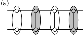
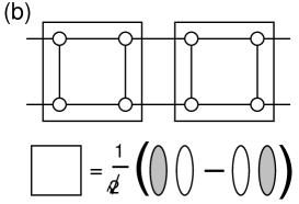
Fig.  3: (a) Physical picture of the plateau A (Néel mechanism). Open and shaded ellipses represent $\psi(0,0)$ and $\psi(1,1)$ states of the rung pairs ($|\Downarrow\rangle$ and $|\Uparrow\rangle$ in the $T$ picture), respectively. (b) Physical picture of the plateau B (dimer mechanism).

The physical pictures of these two plateau states are shown in Fig.3. As is clear from Fig.3, both plateau states are doubly degenerate due to the spontaneous symmetry breaking. Then the period of the state is $Q=2$ in both plateau states, from which we see the realization of the necessary condition eq.(2). The transition from the no-plateau state to the plateau A or B state (in the language of $T$, from the spin-fluid state to the Néel or dimer state) is of the Berezinskii-Kosterlitz-Thouless${}^{\hbox{\immediate{\bf{?}},\penalty 1000\hskip 0.91003pt plus 0.70004pt minus 0.70004pt{\bf{?}})}}$ (BKT) type.${}^{\hbox{\immediate{?},\penalty 1000\hskip 0.91003pt plus 0.70004pt minus 0.70004pt{?})}}$ In general case $J_{2},J_{3}>0$, the transition from the plateau A state to the plateau B state may occur, which has the Gaussian universality.${}^{\hbox{\immediate{?},\penalty 1000\hskip 0.91003pt plus 0.70004pt minus 0.70004pt{?})}}$

We have performed numerical diagonalization by Lanczos method up to 16 spins for the $S=1$ model with $J_{2}$ and/or $J_{3}$ to confirm to existence of two plateaux, predicted by use of the degenerate perturbation theory. As already stated, the transition from the no-plateau state to the plateau A or B state is of the BKT type, of which boundary is very difficult to determine from the numerical data when the conventional methods are used. This is mainly due to the logarithmic size corrections associated with the BKT transition. We have used the level spectroscopy method,${}^{\hbox{\immediate{?},\penalty 1000\hskip 0.91003pt plus 0.70004pt minus 0.70004pt{?},\penalty 1000\hskip 0.91003pt plus 0.70004pt minus 0.70004pt{?},\penalty 1000\hskip 0.91003pt plus 0.70004pt minus 0.70004pt{\bf{?}},\penalty 1000\hskip 0.91003pt plus 0.70004pt minus 0.70004pt{?},\penalty 1000\hskip 0.91003pt plus 0.70004pt minus 0.70004pt{\bf{?}})}}$ by use of which the BKT phase boundary can be determined free from the most dominant logarithmic size corrections. In the level spectroscopy method, we use three excitations defined by (for simplicity we are writing the $L=4n$ case, $n$ being an integer)

$$\Delta_{1} \equiv \frac{1}{2}\left\{E_{0}\left(L,{\frac{L}{2}}+1,\pi\right)+E_{0}\left(L,{\frac{L}{2}}-1,\pi\right)\right\}$$ (12)

$$-E_{0}\left(L,{\frac{L}{2}},0\right),$$

$$\Delta_{0\rm A} \equiv E_{\rm A}\left(L,{\frac{L}{2}},\pi\right)-E_{0}\left(L,{\frac{L}{2}},0\right)$$ (13)

$$\Delta_{0\rm B} \equiv E_{\rm B}\left(L,{\frac{L}{2}},\pi\right)-E_{0}\left(L,{\frac{L}{2}},0\right)$$ (14)

where $E_{0}(L,M,k)$ means the lowest eigenvalue of the $S=1$ ladder Hamiltonian in the subspace where the eigenvalue of the operator $S_{\rm tot}^{z}\equiv\sum_{l}\sum_{j}S^{z}_{l,j}$ is $M$ with the momentum $k$ and system size $L=4n$ under the periodic boundary condition. $E_{0}(L,L/2,0)$ is nothing but the ground state energy. $E_{0\rm A}$ is the lowest energy with $M=L/2,\,k=\pi$ subspace having the eigenvalue $P=-1$ for the space inversion operation of the rung number $i\to L-i+1$. This excitation is called Néel excitation. We have $P=-1$ for $E_{0\rm B}$, which is named dimer excitation. In the no-plateau state, plateau A state and plateau B state, the lowest excitations should be $\Delta_{1}$, $\Delta{0\rm A}$ and $\Delta_{0\rm B}$, respectively. Thus the boundaries between these three phases can be determined from the crossing points among these three excitations with sweeping the coupling constants.${}^{\hbox{\immediate{?})}}$

Fig.  4: The $M_{\rm s}/4$ plateau phase diagram (a) on the $\tilde{J}_{1}-\tilde{J}_{2}$ plane when $J_{3}=0$, and (b) on the $\tilde{J}_{1}-\tilde{J}_{3}$ plane when $J_{2}=0$. Here $\tilde{J}_{i}\equiv J_{i}/J_{\perp}$ for $i=1,2,3$. The closed diamonds represent the BKT phase boundaries and open circles the first order phase boundaries.

Fig.  5: (a) Classical picture of (a) the no-plateau 1 state, and (b) no plateau 2 state.

By use of the level spectroscopy, we obtain the $M_{\rm s}/4$ plateau phase diagrams in Fig.4. The estimated error bars of the boundary points are much smaller than the size of marks. The line symmetry with respect to the line $\tilde{J}_{2}=\tilde{J}_{1}$ in Fig.4(a) is due to the equivalence of the model for interchanging $J_{1}\leftrightarrow J_{2}$ when $J_{3}=0$. The slope of the BKT lines near the origin are very close to the predicted values, $13/19$ in Fig.4(a) and $0.31$ in Fig.4(b), which confirms the high reliability of our analysis of the numerical data by use of the level spectroscopy method. In Fig.4(a), there are two no-plateau phases,${}^{\hbox{\immediate{?},\penalty 1000\hskip 0.91003pt plus 0.70004pt minus 0.70004pt{?},\penalty 1000\hskip 0.91003pt plus 0.70004pt minus 0.70004pt{\bf{?}})}}$ of which classical pictures are shown in Fig.5. Note that the long range order is destroyed by quantum fluctuations in no-plateau states. The boundaries between two no-plateau states are determined by the crossing of the ground state.

Following the present study, the critical value of $J_{3}$ for the realization of the plateau when $J_{2}=0$ is smaller than that of $J_{2}$ when $J_{3}=0$, irrespective of the value of $J_{1}$. Furthermore the plateau B phase can appear for any value of $\tilde{J}_{1}$, although the plateau A cannot be realized for larger values of $\tilde{J}_{1}$. Thus the plateau B is easier to be realized than the plateau A.

One may think that there should exist dashed-line interactions in Fig.6(a). The model of Fig.6(a) has four bond-alternating $S=1/2$ chains. At a glance, the unit cell seems to consist of eight $S=1/2$ spins, which may brings about the $M_{\rm s}/4$ plateau without any spontaneous symmetry breaking. However, the model of Fig.6(a) can be re-drawn in the plane form of Fig.6(b), indicating that the unit cell is still composed of four $S=1/2$ spins. Thus this new interaction cannot be the direct reason for the $M_{\rm s}/4$ plateau. In fact, in the degenerate perturbation theory used in this letter, this new interaction only modifies $J_{\rm eff}^{xy}$ and $J_{\rm eff}^{z}$ in eq.(7) without changing their ratio $\Delta_{\rm eff}=J_{\rm eff}^{xy}/J_{\rm eff}^{z}$. A similar situation can be found in two-leg bond-alternating ladder investigated by Cabra and Grynberg.${}^{\hbox{\immediate{\bf{?}})}}$

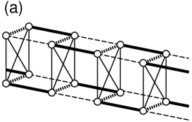
Fig.  6: (a) Picture of four bond-alternating $S=1/2$ chains. (b) Plane type illustration of (a). The unit cell consists of four $S=1/2$ spins.

In conclusion, we have investigated the $M_{\rm s}/4$ plateau of the $S=1$ spin ladder, proposing two mechanisms for the plateau. We have also clarified the plateau-no plateau phase diagram by use of the degenerate perturbation theory, and the level spectroscopy analysis of the numerical diagonalization data. The full study of the magnetization process of the present model will be published elsewhere.

References

• [1] K. Katoh, Y. Hosokoshi, K. Inoue and T. Goto: J. Phys. Soc. Jpn. 69 (2000) 1008.
• [2] T. Goto, M. I. Bartashevich, Y. Hosokoshi, K. Kato, and K. Inoue: to appear in Physica B.
• [3] M. Oshikawa, M. Yamanaka, and I. Affleck: Phys. Rev. Lett. 78 (1997) 1984.
• [4] T. Tonegawa, T. Nishida and M. Kaburagi: Physica B 246-247 (1998) 368.
• [5] K. Totsuka: Phys. Rev. B57 (1998) 3435.
• [6] T. Tonegawa, K. Okamoto and M. Kaburagi; to appear in Physica B.
• [7] F. Mila: Eur. Phys. J. B6 (1998) 201.
• [8] N. Okazaki, J. Miyoshi and T. Sakai: J. Phys. Soc. Jpn. 69 (2000) 37.
• [9] N. Okazaki, K. Okamoto and T. Sakai: J. Phys. Soc. Jpn. 69 (2000) 2419.
• [10] K. Okamoto: in preparation.
• [11] T. Tonegawa, K. Okamoto, T. Hikihara, Y. Takahashi and M. Kaburagi: to appear in J. Phys. Chem. Solids.
• [12] A. Honecker and A. LΓ€uchli: cond-mat/0005398
• [13] K. Nomura and K. Okamoto: J. Phys. Soc. Jpn. 62 (1993) 1123.
• [14] K. Nomura and K. Okamoto: J. Phys. A: Math. Gen. 27 (1994) 5773.
• [15] V. L. Berezinski, Zh. Eksp. Teor. Fiz. 59 (1970) 907; Sov. Phys. JETP 32 (1971) 493.
• [16] J. M. Kosterlitz and D. J. Thouless: J. Phys. C 6 (1973) 1181.
• [17] K. Okamoto and K. Nomura: Phys. Lett. A 162 (1992) 433.
• [18] K. Nomura: J. Phys. A: Math. Gen. 28 (1995) 5451.
• [19] T. Sakai and N. Okazaki: J. Appl. Phys. 87 (2000) 5893.
• [20] D. C. Cabra and M. D. Grynberg: Phys. Rev. Lett. 82 (1999) 1768.