[

Effective Lorentz Force due to Small-angle Impurity Scattering: Magnetotransport in High-$T_{c}$ Superconductors

Abstract

We show that a scattering rate which varies with angle around the Fermi surface has the same effect as a periodic Lorentz force on magnetotransport coefficients. This effect, together with the marginal Fermi liquid inelastic scattering rate gives a quantitative explanation of the temperature dependence and the magnitude of the observed Hall effect and magnetoresistance with just the measured zero-field resistivity as input.

]

The temperature dependence of the transport properties in the normal state of high-temperature superconductors [1] are unlike Landau Fermi liquids. Most of the observed anomalies near the composition for the highest $T_{c}$ follow from the hypothesis of a scale-invariant fluctuation spectrum [2], characteristic of a quantum critical point, which is a function of $\omega/T$ and which has negligible momentum dependence over most of the Brillouin zone. One of the principal predictions of this hypothesis is that at low energies the inelastic part of the single-particle relaxation rate has the marginal Fermi liquid (MFL) form $\lambda T$ with coefficient $\lambda$ having negligible momentum dependence either along or perpendicular to the Fermi surface. This prediction has been verified in detail in recent angle-resolved photoemission (ARPES) measurements [3].

However, the observed anomalies in the magnetotransport [4, 5, 6] do not follow from the MFL hypothesis. Various explanations [7, 8] have been advanced for these anomalies, none of which are independently supported by other experiments, and in some cases are in conflict with photoemission experiments.

The ARPES experiments [3] have revealed, besides the inelastic contribution to the single-particle self energy, an elastic contribution (independent of temperature or frequency) which is angle-dependent around the Fermi surface, increasing by about a factor of 4 from the $(\pi,\pi)$ to the $(\pi,0)$ directions. Thus the total self energy at low frequency has an imaginary part of the form

$${\rm Im}\>\Sigma({\vec{k}},T)\ =\ \Gamma_{0}(\hat{k})+\lambda T,$$ (1)

The anisotropic elastic part, $\Gamma_{0}(\hat{k})$, has been ascribed to small-angle scattering from dopant impurities lying between the Cu-O planes [9]. If $d$ is the characteristic distance of such impurities from a Cu-O plane the electron scattering at a point $\hat{k}$ on the Fermi-surface is confined to small momentum transfers $\delta k\leq d^{-1}$. Then, on the Fermi surface, the scattering rate at a point $\hat{k}$ is proportional to $\delta k$, to the local density of states and to the forward scattering matrix element at $\hat{k}$. The latter two quantities can be anisotropic especially near a crossover or a transition to an anisotropic pseudogap state. We do not address the sources of anisotropy here and simply take $\Gamma_{0}(\hat{k})$ from experiment and follow the consequences.

In a planar lattice of square symmetry, the anisotropic scattering rate $\Gamma_{0}(\hat{k})$, has a four-fold symmetry as one goes around the Fermi surface. Since it is largest in the $(\pi,0)$ directions [9], a non-equilibrium particle distribution is skewed away from the region of the Fermi surface near the $(\pi,0)$ directions toward the $(\pi,\pi)$ directions. We show that this acts as an effective magnetic field, perpendicular to the planes which changes sign at every multiple of $\pi/4$ in going around the Fermi surface. Together with the MFL scattering rate, such a skewed distribution gives an anomalous contribution to the magnetotransport properties with the experimentally observed temperature dependences. Using just the measured dc resistance, we can explain the observations quantitatively. We also explain the observed variation in the anomalous magnetotransport properties due to impurities like Zn which replace Cu in the plane and cause angle-independent ($s$-wave) scattering.

The skewed non-equilibrium distribution is apparent from the (formal) solution of the linearized Boltzmann equation. Let $g({\bf k})$ be the deviation from the equilibrium distribution $f_{0}({\bf k})$ due to the applied uniform steady state electric and magnetic fields ${\bf E}$ and ${\bf B}$. It is formally given by [8]

$$g({\bf k})=e\sum_{\bf k^{\prime}}\ A^{-1}_{{\bf k},{\bf k}^{\prime}}\left[{\bf E}\cdot{\bf v}_{{\bf k}^{\prime}}\left(-\frac{\partial f_{0}}{\partial\epsilon_{{\bf k}^{\prime}}}\right)\right],$$ (2)

where

$$A_{{\bf k},{\bf k}^{\prime}}=\left[{1\over\tau({\bf k})}\ +{e\over\hbar c}\>{\bf v}_{\bf k}\times{\bf B}\cdot\nabla_{\bf k}\right]\delta_{{\bf k},{\bf k}^{\prime}}-C_{{\bf k},{\bf k}^{\prime}}.$$ (3)

Here $C_{{\bf k},{\bf k}^{\prime}}$ is the “scattering-in” term in the collision operator for the Boltzmann equation and $1/\tau({\bf k})=\sum_{{\bf k}^{\prime}}C_{{\bf k},{\bf k}^{\prime}}$, is the “scattering-out” term equal to the single-particle relaxation rate. From Eqs. (3,4) It is evident that the distribution $g({\bf k})$ is not merely determined by the energy of the state ${\bf k}$ but also by the anisotropy of the scattering. The distribution is depleted in directions of large net scattering and augmented in directions of small net scattering.

We shall calculate the conductivities for $\omega\ll T$ using the single-particle scattering rate of Eq. (1). The conductivity tensor is

$$\sigma^{\mu\nu}=e^{2}\sum_{{\bf k},{\bf k}^{\prime}}\>v_{\mu,{\bf k}}\ A_{\bf k,\bf k^{\prime}}^{-1}\>v_{\nu,{\bf k}}\left(-{\partial f_{0}\over\partial\epsilon_{\bf k^{\prime}}}\right).$$ (4)

We expand $A^{-1}$ from Eq. (3) in powers of $\bf B$ [8]:

$$A^{-1}={\cal T} - {\cal T}({\bf v}\times{\bf B\cdot\nabla})\,{\cal T}$$ (5)

$$+ {\cal T}({\bf v\times B\cdot\nabla})\,{\cal T}\,({\bf v\times B\cdot\nabla})\,{\cal T},$$ (6)

where, from Eq. (2.12) of Ref. [8], it follows that

$${\cal T}({\bf k},{\bf k}^{\prime})=\tau(\bf k)\delta_{{\bf k},{\bf k}^{\prime}}+\sum_{{\bf k}^{\prime\prime}}\tau(\bf k)C_{{\bf k},{\bf k}^{\prime\prime}}{\cal T}({\bf k}^{\prime\prime},{\bf k}^{\prime}).$$ (7)

The first term in $A^{-1}$ gives the dc conductivity, $\sigma^{xx}$ etc., the second the Hall conductivity $\sigma^{xy}$ and the magnetoconductivity may be calculated from the third term.

Let $\theta,\,\theta^{\prime}$ be the angles of ${\bf k,\,k}^{\prime}$ with respect to the $k_{x}$ axis in reciprocal space. The use of the Boltzmann formulation and the presence of $-\partial f_{0}/\partial\epsilon$ in Eq. (2) essentially restricts all variables to the Fermi surface; it implies that all the scattering is quasielastic. We take $C_{{\bf k},{\bf k}^{\prime}}$ to be composed of three parts:

$$C_{{\bf k},{\bf k}^{\prime}}=2\pi\delta(\epsilon_{\bf k}-\epsilon_{{\bf k}^{\prime}})\left(|U_{M}|^{2}+|u_{i}(\theta,\theta^{\prime})|^{2}+|U_{i}|^{2}\right).$$ (8)

The first contribution, due to MFL, is parameterized by an angle independent quasielastic scattering proportional to $T$. The second and the third terms are due to small angle and large angle elastic impurity scattering respectively. The effect of $U_{i}$ is simply to add a temperature independent scattering rate to the MFL scattering rate. $u_{i}(\theta,\theta^{\prime})$ is a symmetric function of $\theta$ and $\theta^{\prime}$ sharply peaked at $\theta^{\prime}=\theta$ with a small characteristic width $\theta_{c}(\theta)$. Then to order $\theta_{c}^{3}$ the single particle scattering rate is

$$\tau^{-1}(\theta) = \tau_{M}^{-1}+\tau_{i}^{-1}(\theta)$$ (9)

$$\tau_{i}^{-1}(\theta) = \theta_{c}|u_{i}(\theta,\theta)|^{2}N(\theta)$$ (11)

$$+\left(\frac{\theta_{c}^{3}}{24}\right){\partial^{2}\over\partial\theta^{\prime 2}}\left[|u_{i}(\theta,\theta^{\prime})|^{2}N(\theta^{\prime})\right]_{\theta^{\prime}=\theta},$$

where $N(\theta)$ is the density of states per radian at the Fermi surface at angle $\theta$ and $\tau_{M}^{-1}$ is the sum of the MFL scattering rate proportional to $T$ and the large angle impurity scattering rate.

Given the quasielastic $C_{{\bf k},{\bf k}^{\prime}}$, one may integrate over the energy variable $\epsilon_{\bf k^{\prime}}$ (i.e. perpendicular to the Fermi surface) in Eq. (4). To evaluate the conductivities, it is convenient to define the operator $\hat{\tau}$ by

$$\hat{\tau}(\theta)v_{\alpha}(\theta)(-\partial f_{0}/\partial\epsilon_{{\bf k}}) \equiv \sum_{{\bf k}^{\prime}}{\cal T}_{{\bf k,k}^{\prime}}v_{\alpha,{\bf k}^{\prime}}(-\partial f_{0}/\partial\epsilon_{{\bf k}^{\prime}})$$ (12)

$$= {1\over 2\pi}\int d\theta^{\prime}N(\theta^{\prime}){\cal T}(\theta,\theta^{\prime})v_{\alpha}(\theta^{\prime}),$$ (13)

where the $v_{\alpha}$ are the Fermi surface velocity components.

From Eqs. (6,7) it follows that

$$\hat{\tau}(\theta)v_{\mu}(\theta)\ =\ \tau(\theta)v_{\mu}(\theta)+{\hat{\rm t}}v_{\mu}(\theta)$$ (14)

where

$${\hat{\rm t}}v_{\mu}(\theta)\equiv{\tau(\theta)\over 2\pi}\int d\theta^{\prime}N(\theta^{\prime})\ C(\theta,\theta^{\prime})\hat{\tau}(\theta^{\prime})v_{\mu}(\theta^{\prime}),$$ (15)

where $C(\theta,\theta^{\prime})$ is Eq. (7) without the energy $\delta$-function.

Now ${\hat{\rm t}}v_{\mu}(\theta)=0$ for momentum-independent scattering. This is simply the traditional result of no vertex corrections for such scattering. Therefore, in Eq. (12) we use only the small-angle scattering part in $C$ and find

$$\frac{{\hat{\rm t}}v_{\mu}(\theta)}{\tau(\theta)} = \left[{1\over\tau_{i}(\theta)}\hat{\tau}(\theta)v_{\mu}(\theta)\right]$$ (16)

$$- \left({\theta_{c}^{3}\over 24}\right){\partial^{2}\over\partial\theta^{\prime 2}}\left[N(\theta^{\prime})~{}|u_{i}(\theta,\theta^{\prime})|^{2}\right]_{\theta^{\prime}=\theta}\hat{\tau}(\theta)v_{\mu}(\theta)$$ (17)

$$+ \left({\theta_{c}^{3}\over 24}\right){\partial^{2}\over\partial\theta^{\prime 2}}\left[N(\theta^{\prime})~{}|u_{i}(\theta,\theta^{\prime})|^{2}~{}\hat{\tau}(\theta^{\prime})v_{\mu}(\theta^{\prime})\right]_{\theta^{\prime}=\theta}.$$ (18)

Then

$${\hat{\tau}}v_{\mu}=\tau\left\{v_{\mu}+\left[{1\over\tau_{i}}-\left({1\over\tau_{u}}\right)^{\prime\prime}\right]{\hat{\tau}}v_{\mu}+\left[{1\over\tau_{u}}{\hat{\tau}}v_{\mu}\right]^{\prime\prime}\right\},$$ (19)

where primes denote derivatives with respect to $\theta$ and $1/\tau_{u}$ is the impurity scattering contribution to the transport scattering rate and is given, to leading non-trivial order in $\theta_{c}$, by

$${1\over\tau_{u}(\theta)}\simeq(\theta_{c}^{2}/24){1\over\tau_{i}(\theta)}$$ (20)

That small angle impurity scattering has much less effect on the transport rate [9] than on the single-particle scattering rate is evident in Eq. (15).

In Eq. (14), derivatives of $\hat{\tau}(\theta)$ lead to corrections of higher order in $\theta_{c}$ compared to the other terms and may be neglected. Therefore, we have

$$\left({1\over\tau}-{1\over\tau_{i}}\,\right){\hat{\tau}}\,v_{\mu}=v_{\mu}+2\left({1\over\tau_{u}}\right)^{\prime}{\hat{\tau}}\,v_{\mu}^{\prime}+{1\over\tau_{u}}{\hat{\tau}}\,v_{\mu}^{\prime\prime},$$ (21)

The derivatives of the Fermi velocity components may be written as $v_{\mu}^{\prime}=\sum_{\nu}b_{\mu\nu}(\theta)v_{\nu}$. The relevant two-dimensional Fermi surface has four-fold symmetry. Let $\phi(\theta)$ be the angle of the Fermi velocity $\vec{v}(\theta)$ with respect to the $k_{x}$ axis in the Brillouin zone. The precise form of $b_{\mu\nu}$ depends on Fermi surface details. For example, for the case that $|v|$ is constant, $v_{x}^{\prime}=-(d\phi/d\theta)v_{y}$ and $v_{y}^{\prime}=(d\phi/d\theta)v_{x}$. It may be verified that $(v_{x},v_{y})$ form an orthogonal basis for the irreducible two-dimensional representation of the group of the square. All other quantities which enter into the coefficients $b_{\mu\nu}(\theta)$ and elsewhere, e.g. $|\vec{v}|,\,\,d\phi/d\theta,\,d(1/\tau_{u})/d\theta,\ldots$ transform according to the identity. We shall use these facts below to eliminate certain integrals on symmetry grounds.

The solution to the coupled equations Eq. (16) has the following form:

$${\hat{\tau}}{\vec{v}}=\tau_{t}\,\left[{\vec{v}}-(\tau_{t}/\tau_{p})\,{\vec{v}}\times{\hat{\bf z}}\right]$$ (22)

where $\hat{\bf z}$ is the unit vector normal to the Cu-O plane. The scattering rates $1/\tau_{t}$ and $1/\tau_{p}$ depend on the precise shape of the Fermi surface. To simplify what follows, we take the case that the Fermi speed is constant over the Fermi surface. In that case, there is a single coefficient $b_{\mu\nu}$ which is just $\phi^{\prime}=d\phi/d\theta$. In addition, we keep only the leading orders in $\theta_{c}$. Then, the $\tau$s are determined by

$${1\over\tau_{t}} = {1\over\tau}-{1\over\tau_{i}}+(\phi^{\prime})^{2}{1\over\tau_{u}}={1\over\tau_{M}}+(\phi^{\prime})^{2}{1\over\tau_{u}}$$ (23)

$${1\over\tau_{p}} = 2~{}(\phi^{\prime})~{}{d\over d\theta}\left({1\over\tau_{u}}\right)+(\phi^{\prime\prime})~{}{1\over\tau_{u}}.$$ (24)

The structure of Eq. (17) shows that the deviation of the distribution from equilibrium which is determined by ${\hat{\tau}}v$ has a skew character. Thus, there is an effective Lorentz force which rotates the carrier distribution into the directions of weak small-angle scattering. Because $d(1/\tau_{u})/d\theta$ changes sign at each $\theta=n\pi/4$, carriers moving on the Fermi surface experience an effective magnetic field which changes sign eight times around the Fermi surface. This has important consequences for $\sigma^{xy}$.

Knowing $\hat{\tau}\,v$, we evaluate $\sigma^{xx}$ from Eqs. (4,5,11):

$$\sigma^{xx} = e^{2}\sum_{{\bf k}{\bf k}^{\prime}}v_{x}({\bf k}){\cal T}_{{\bf k}{\bf k}^{\prime}}v_{x}({\bf k}^{\prime})(-\partial f_{0}/\partial\epsilon^{\prime})$$ (25)

$$= (e^{2}/2\pi)\int d\theta N(\theta)v_{x}(\theta)[{\hat{\tau}}(\theta)v_{x}(\theta)].$$ (26)

Using Eq. (17), we obtain

$$\sigma^{xx}=(e^{2}/2\pi)\int d\theta N(\theta)[v_{x}(\theta)]^{2}\tau_{t}(\theta).$$ (27)

For $\sigma_{xy}$, we use Eq. (17) again and find

$$\sigma^{xy}={e^{3}B\over 4\pi^{2}c}\int d\theta\,\tau_{t}(v_{x}-{\tau_{t}\over\tau_{p}}v_{y}){\partial\over\partial\theta}\left[\tau_{t}(v_{y}+{\tau_{t}\over\tau_{p}}v_{x})\right].$$ (28)

Finally, we get, to leading orders in $\theta_{c}$,

$$\sigma^{xy}={e^{3}B\over 4\pi^{2}c}\int d\theta[\phi^{\prime}\,\tau_{t}^{2}v_{x}^{2}+\tau_{t}^{3}\,(\partial\tau_{p}^{-1}/\partial\theta)\,v_{x}^{2}].$$ (29)

Eqs. (21,23) are our main results. From them we may determine the Hall angle $\Theta_{H}={\rm tan}^{-1}(\sigma^{xy}/\sigma^{xx})$. We find

$$\tan\Theta_{H}=\tan(\Theta_{H})_{0}+\omega_{H}\,\overline{\tau^{2}_{t}(\tau_{p}^{-1})^{\prime}}$$ (30)

where the first term is the customary contribution and in the new contribution which we have found, the overbar represents an appropriate average over the Fermi surface according to Eqs. (21,23). Our principal finding is that new contribution has the temperature dependence of the resistivity relaxation time $\tau_{t}$ squared.

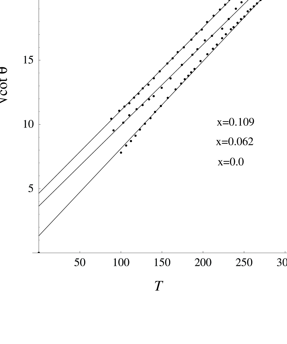
FIG. 1.: Hall angle data for three concentrations of Zn in YBCO. The straight lines are least-squares fits to the data (replotted from Chien et al [4]) for $\sqrt{\cot\theta_{H}(T)}$ vs $T$.

The customary contribution depends on the details of the band structure. For YBCO near optimum composition, band-structure calculations [10] find for the Hall constant a value which is about five times smaller than what is actually measured. The customary contribution to $\tan(\Theta_{H})$ is then at least five times smaller than the measured value and is probably even smaller due to Fermi-liquid effects. Then with neglect of the customary term, our conclusion is that $(\cot\Theta_{H})^{1/2}$ should be proportional to $\tau^{-1}_{t}$ which is independently measured by the zero-field resistivity. As seen in Eq. (18), $\tau^{-1}_{t}$ contains an impurity-independent part with MFL linear $T$ dependence and a $T$-independent part depending on impurity content. Fig. 1 shows the comparison for samples with varying concentration, $x$, of Zn impurities in an applied magnetic field of 8 Tesla. The straight lines are least-square fits to the data from Chien et al [4]. The data is consistent with a slope independent of $x$, as predicted. The increase of the intercept with $x$ is due to the increased large-angle scattering from in-plane impurities. For well-prepared samples, the ratio of resistivity (hence of $1/\tau_{t}$) at 100 K to the 0 K extrapolated value is usually about 10. This is consistent with the present analysis which gives $\sim 7$ for the corresponding ratio for $[\cot\Theta_{H}(T)]^{1/2}$ from the data. The magnitudes of the various terms which enter the transport coefficients depend very sensitively on the shape of the Fermi surface and the precise variation with angle of the impurity scattering rate $1/\tau_{i}$. To make further estimates, we adopted a model Fermi surface similar to the measured one. We estimate the small-angle parameter $\theta_{c}$: The extrapolated resistivity at $T=0$K is determined by $1/\tau_{u}=(\theta_{c}^{2}/24)(1/\tau_{i})$ and that at $T=100$K is determined by $1/\tau_{M}(100$K). Using the ARPES-measured $1/\tau_{i}$ and $1/\tau_{M}$ and a typical resistivity ratio $\rho(100$K)/$\rho(0$K) of 9, we find $\theta_{c}^{2}/24\approx.01$. We use the measured $1/\tau_{M}$ and the above-determined $1/\tau_{u}$ to compare the new contribution to $\sigma^{xy}$ to the conventional one - i.e. the ratio of the integrals of the second to the first term in square brackets in Eq. (23). For the model Fermi surface, we found the new contribution to be almost two orders of magnitude larger that the conventional piece, even without invoking the band-structure result mentioned earlier. We have thus given a demonstration-in-principle of our principal finding. Since the effects of the anisotropic small-angle scattering can be quite large, it is natural to ask whether higher order terms in $\theta_{c}^{2}/24$ are important. Using the same model, we find them to be less that 3% of the leading term.

Ong [11] has derived a relation between the magnetoresistance and moments of the fluctuations of the Hall angle over the Fermi surface in two dimensions. This relationship continues to hold in the present case. For small Hall angle, an order of magnitude estimate is

$$(\Delta\rho/\rho)(B)\sim\Theta^{2}_{H},$$ (31)

Using similar arguments to those of the previous paragraph, our result for the Hall angle gives the measured temperature dependence of the magnetoresistance[4] as well as order of magnitude numerical agreement.

We extend the theory to low frequencies ($\omega\tau_{t}\ll 1$) by means of the replacement $1/\tau_{M}\rightarrow i\omega+\tau^{-1}_{M}$ so that $\cot\theta_{H}\propto(i\omega+\tau_{t}^{-1})^{2}$. The observed low-frequency behavior of the real and imaginary parts of the Hall angle [6] then follow.

Two properties which follow from the MFL phenomenology and experiment are crucial in the resolution of the puzzle of the magnetotransport anomalies in the high-$T_{c}$ superconductors: the observed angle-dependent elastic scattering and the angle-independent T-linear (MFL) inelastic scattering. The latter is obtained as scattering off a scale invariant fluctuation spectrum [2]. Indeed, essentially all of the principal normal state anomalies in the high-$T_{c}$ superconductors near optimal composition have now been shown to follow from the MFL fluctuation spectrum. Furthermore, since the interaction vertices which give the normal state scattering rates also contribute to Cooper pairing, we expect that these fluctuations, which have the right magnitude of cut-off frequency $\omega_{c}$ and coupling constant $\lambda$, mediate high-$T_{c}$ superconductivity.

The authors thank the Aspen Center for Physics where part of this work was carried out. EA was supported in part by NSF grant DMR99-76665.

REFERENCES

• [1] For reviews see Physical Properties of High Temperature Superconductors, Edited by D.M. Ginsberg [World Scientific, Singapore, Vol. I (1989), Vol. II (1990), Vol. III (1992), Vol. IV (1994)].
• [2] C. M. Varma, P.B. Littlewood, S. Schmitt-Rink, E. Abrahams and A.E. Ruckenstein, Phys. Rev. Lett. 63, 1996 (1989); C. M. Varma, Int. J. Mod. Physics 3, 2083 (1989).
• [3] T. Valla et al., Science 285, 2110 (1999); cond-mat/0003407v2; A. Kaminsky et al., Phys. Rev. Letters, 84, 1788 (2000); A. Kaminsky and J.C. Campuzano (private communication) - some of the pertinent data is reproduced in Ref.Β [9]
• [4] T.R. Chien, Z.Z. Wang and N.P. Ong, Phys. Rev. Lett. 67, 2088 (1994); J.M. Harris et al Phys. Rev. B46, 14293 (1992), Phys. Rev. Lett. 75, 1391 (1996); A. Carrington, A.P. Mackenzie, C.T. Lin and J.R. Cooper, Phys. Rev. Lett. 69, 2855 (1992).
• [5] H.Y. Hwang et al., Phys. Rev. Lett. 72, 2636 (1994)
• [6] H.D. Drew et al, J. Phys. Cond. Mat. 8, 10037 (1996) and private communication.
• [7] P.W. Anderson, Phys. Rev. Lett. 67, 2092 (1991); A. Carrington, A.P. Mackenzie, C.T. Lin and J.R. Cooper, Phys. Rev. Lett. 69, 2855 (1992); P. Coleman, A.J.Schofield and A.M.Tsvelik, Phys. Rev. Lett. 76, 1329 (1996); B.P. Stojkovic and D. Pines, Phys. Rev. Lett. 76, 811 (1996); L.B. Ioffe, V. Kalmeyer and P.B. Wiegmann, Phys. Rev. B43, 1219 (1991); L.B. Ioffe and A.J. Millis, Phys. Rev. B56,11631 (1998); E. Abrahams, J. Phys. I France 6, 2191 (1996).
• [8] G. Kotliar, A. M. Sengupta and C. M. Varma, Phys. Rev. B53, 3573 (1996).
• [9] E.Β Abrahams and C.M.Β Varma, Proc.Β Nat.Β Acad.Β Sci.Β 97, 5714 (2000).
• [10] P.B.Β Allen, W.E.Β Pickett and H.Β Krakauer, Phys.Β Rev.Β B37, 7482 (1988).
• [11] N.P. Ong, Phys. Rev. B43, 193 (1991). This result was subsequently derived within the present Boltzmann formulation in Ref. [8].