[

Is there a vortex-glass transition in high-temperature superconductors?

Abstract

We show that DC voltage versus current measurements of a $\mathrm{YBa_{2}Cu_{3}O_{7-\delta}}$ micro-bridge in a magnetic field can be collapsed onto scaling functions proposed by Fisher, Fisher, and Huse, as is widely reported in the literature. We find, however, that good data collapse is achieved for a wide range of critical exponents and temperatures. These results strongly suggest that agreement with scaling alone does not prove the existence of a phase transition. We propose a criterion to determine if the data collapse is valid, and thus if a phase transition occurs. To our knowledge, none of the data reported in the literature meet our criterion.

]

One of the more remarkable consequences of research on high-temperature superconductors is a new picture of the normal to superconducting transition in a magnetic field. While the mean-field Ginzburg-Landau description had been viewed as adequate for low-temperature superconductors, a consensus has emerged [2, 3, 4, 5, 6] that a vortex-glass transition occurs in the high-temperature superconductors. The strongest evidence has come from $voltage$ vs. $current$ ($I-V$) measurements [7] where data can be collapsed onto two scaling functions, as proposed by Fisher, Fisher, and Huse (FFH) [8].

Despite a strong consensus that this data collapse implies the transition, some workers have suggested that the apparent agreement with scaling is misleading [9, 10]. Some simulations of $I-V$ curves which are based on models without a phase transition have also been shown to collapse onto scaling functions within limited voltage ranges.

It has been countered [5] that the simulations invoke highly unphysical parameters in order to obtain “scalable” data which resemble actual measurements. Moreover, the critical exponents found from the simulated data [9, 10] differ drastically from the ones obtained experimentally. Fueling the debate still further have been some recent attempts at measuring $I-V$ curves over larger voltage ranges, where critical exponents have been found [6, 11] which approach those resulting from the controversial simulations [9, 10].

Furthermore, it has recently been proposed [12] that a true phase transition, such as the vortex-glass transition, does not actually occur. This “window-glass” scenario is more like a conventional glass transition, where the dynamics slow down considerably over a small temperature range, but correlation length scales do not strictly diverge. If a superconductor were to behave in this way, the linear resistance could rapidly decrease upon lowering temperature, but would not become zero. A small but non-vanishing linear resistance has also been predicted by theoretical studies that incorporate screening [13, 14].

Granting all this, we do not see how this issue can be resolved through the use of simulated $I-V$ curves as in Refs. [9] and [10]. Simply showing that simulated data from a model without a transition scales does not demonstrate that the measurements scale for the same reason. The scaling interpretation of measurements may still be valid.

What is needed is an unambiguous signature in the data that can be used to make a valid claim for a transition. The purpose of this letter is to propose such a criterion and to show that it is necessary. We propose that a criterion for determining whether data supports a nonarbitrary choice of the critical parameters is that $\log(voltage)$ vs. $\log(current)$ isotherms equally distanced (ie. with equal $\left|(T-T_{g})/T_{g}\right|$) from the critical temperature, $T_{g}$, must have opposite concavities at the same applied currents. This contrasts with previously published data where opposite concavity is seen, but not at the same applied currents.

We begin by showing the difficulties in experimentally demonstrating that a true phase transition exists in a superconductor. We start with a typical scaling analysis of $I-V$ data taken on a $\mathrm{2200\AA}$ thick $\mathrm{YBa_{2}Cu_{3}O_{7-\delta}}$ film laser ablated onto an STO substrate. This sort of film has previously been shown to have transport characteristics which agree with a scaling analysis in externally applied magnetic fields of about 4 tesla [2, 3, 4, 5, 6]. The high quality of our film was verified with x-ray diffraction peaks of predominately c-axis orientation, from an AC susceptibility measurement transition width of 0.2K in zero magnetic field, and through zero field R(T) (inset of Fig. 1) which shows a $T_{C}\approx 91.5K$ and a transition width of about 0.5K. The film was photo-lithographically patterned into a four terminal bridge $8\mu m$ wide by $40\mu m$ long and etched using a dilute solution of phosphoric acid with no noticeable degradation of R(T).

Figure 1 shows $I-V$ measurements taken on our film in a perpendicular magnetic field of 4 tesla. The scaling analysis requires that [8]

$$V\xi^{2+z-D}/I=\chi_{\pm}({I\xi^{D-1}}/{T})$$ (1)

where the dimensionality, $D$, is 3, $z$ is the dynamic critical exponent, $\xi$ is the glass correlation length which is expected to behave as $\left|(T-T_{g})/T_{g}\right|^{-\nu}$, $\nu$ is the correlation-length exponent, and $\chi_{\pm}$ are the scaling functions for above and below the glass transition temperature $T_{g}$.

The parameters of Eq. (1) are found from experimental data in the standard way. First, only those $I-V$ isotherms above $T_{g}$ should show low-current ohmic tails, where ohmic behavior is represented in Fig. 1 by the dashed line on the lower left with a slope of 1. At higher currents the isotherms are non-ohmic, and it is typically presumed that they cross over to power law behavior (ie. straight lines on $log-log$ plots with slope greater than 1).

The thick solid line at 81K is a power-law fit to the isotherm which separates those with low-current ohmic tails from the ones without. This is conventionally designated as $T_{g}$ and the slope of the fitted line on this plot gives the dynamic exponent of $z=5.46$, since $V\propto I^{(z+1)/2}$ is expected at $T_{g}$ from Eq. (1). The static exponent can be found from the low-current ohmic tails, $R_{L}$, which are expected to behave as

$$R_{L}\propto({T/T_{g}}-1)^{\nu(z-1)}.$$ (2)

Using the $z$ and $T_{g}$ found above we plot the $log_{10}$ of both sides of Eq. (2) in the inset of Fig. 2(a). Since scaling predicts that this plot should be a straight line, deviations from this at about 87K determine the extent of the critical region, which is $\pm\mathrm{5.5K}$ from $T_{g}$. Only data lying within this temperature window will be used to test Eq. (1), below.

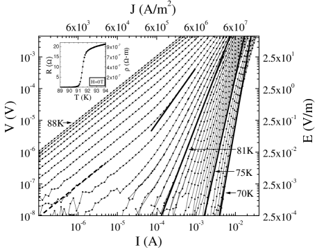
FIG. 1.: $I-V$ isotherms for a $2200\mathrm{\AA}$ thick $\mathrm{YBa_{2}Cu_{3}O_{7-\delta}}$ film in 4 tesla. The dashed line has a slope of one, and represents ohmic behavior, while the solid lines are linear fits to the non-ohmic power law-like regions of various isotherms. The inset shows an R(T) in ambient field.

Data at high currents are also excluded because free flux flow occurs which is not described by scaling [2, 6]. A cut off is conventionally set to the voltage where the critical isotherm begins to deviate towards ohmic behavior, which is seen as a slight decrease in slope at about $10^{-3}V$ in Fig. 1. Plotting all the data in Fig. 1 below this voltage and within the 11K range about 81K, a conventional data collapse is clearly demonstrated in Fig. 2(a) with the critical exponents in good agreement with those reported elsewhere, $z=5.46$ and $\nu=1.5$.

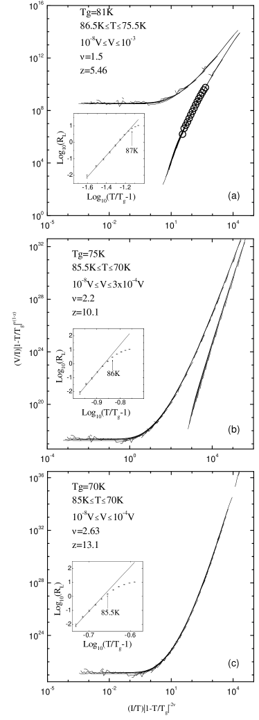
FIG. 2.: Data collapses of the $I-V$ curves of Fig. 1 using various critical parameters with the experimental windows for each one denoted. The conventional analysis is the one shown in (a). The insets show the $R_{L}$ plotted according to Eq. (2)

There is a serious problem with the analysis outlined above. Following Repaci et al. [15], we demonstrate this by plotting the derivatives of the $\log(voltage)$ vs. $\log(current)$ isotherms, which are shown in Fig. 3 as small solid dots. The predicted power-law $I-V$ curve at $T_{g}$ should correspond to a horizontal line in Fig. 3, with a value of $(z+1)/2$. The data, however, peaks at about $7\times 10^{-4}\mathrm{A}$. In fact, all isotherms seem to have a maximum slope at about this current with ohmic tails developing to the left of the peaks. Apparently, the only difference between the isotherms above and below the conventionally determined $T_{g}$ is that the ones at lower temperatures are truncated due to the resolution limit of the experiment before they decrease in slope towards ohmic behavior. This truncation is evident in these derivative plots where the data at lower currents and voltages become noisier.

Since the conventionally chosen critical isotherm does not show any signs of unique power law behavior, we now ask whether it is possible to choose other values for $T_{g}$ which also lead to data collapse. To do this we note that non-ohmic power law-like behavior can be fit to the lower temperature isotherms over at least 4 decades of voltage data. We have demonstrated this in Fig. 1 for the isotherms at 75K and 70K. By repeating the scaling analysis assuming that these two temperatures are the critical isotherms we can again obtain excellent data collapses as is demonstrated in Figs. 2(b) and 2(c).

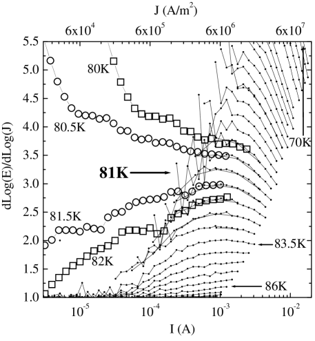
FIG. 3.: $dlog(V)/dlog(I)$ isotherms from Fig. 1 are plotted as small solid dots. The open squares are extrapolated data which are 1K from $T_{g}$ while the open circles are ones 0.5K from $T_{g}$. Both pairs of extrapolated data were extracted from the collapse shown in Fig. 2(a).

When we lower the defined $T_{g}$ by 6K in going from Fig. 2(a) to Fig. 2(b) we need only readjust $z$ and $\nu$ in order to maintain successful data collapse with an even larger critical region (greater than 15K). As shown in Fig. 2(c), $T_{g}$ can even be defined as the lowest temperature of our measurement, where $\chi_{-}$ is not shown because there is no data below 70K.

Now that we have demonstrated that a data collapse does not uniquely determine the critical parameters, we propose a criterion for uniquely determining $T_{g}$, and thus $\nu$ and $z$.

Such a signature is suggested by the scaling functions found from the conventional vortex-glass analysis. To see this it is important to note that each isotherm in Fig. 1 collapses onto only small portions of the scaling functions of Fig. 2. We demonstrate this by plotting only the isotherm at 79K as open circles in Fig. 2(a). In the low current direction of the collapses the isotherms are cut off by the voltage sensitivity floor of the experiment.

We can, however, predict how data at lower voltages would behave if a data collapse is assumed to represent a real transition. We do this by using the temperature for the desired isotherm, a current, and the values of the parameters $\nu$ and $T_{g}$ used in the collapse. This information determines a position along the horizontal axis of Fig. 2(a). Now, by using the vertical axis value of the scaling function along with the $z$ exponent we can solve for the predicted voltage.

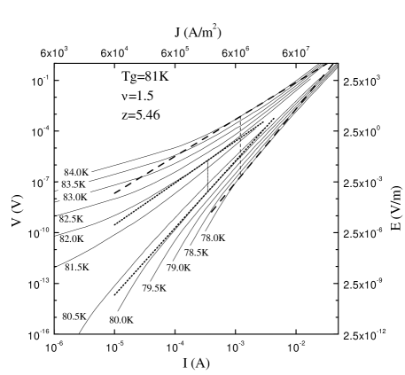
FIG. 4.: Extrapolated $I-V$ data from the collapse of Fig. 2(a). Dashed and dotted lines are tangents drawn to the isotherms in order to demonstrate opposite concavity at common applied currents.

The results of the extrapolation are shown in Fig. 4, with the $I-V$ curves displaying a property not seen in the measured data. For isotherms at equal temperatures away from $T_{g}$ (ie. equal $\left|(T-T_{g})/T_{g}\right|$), opposite concavities are clearly evident at the same current level. We demonstrate this in Fig. 4 with vertical lines which represent constant currents drawn between two different pairs of isotherms. Tangent lines to these isotherms at the intersections clearly show that both pairs have opposite concavity at the same applied currents. The reader can verify that this signature would restrict the assignment of $T_{g}$ to within $\pm\mathrm{0.5K}$ of 81K whether the resolution of the experiment would be at $10^{-16}\mathrm{V}$ or $10^{-10}\mathrm{V}$ [16] by covering the extrapolated data at low voltages.

We demonstrate the striking contrast between this extrapolated data and the real data by plotting the extrapolated ones as open squares and circles on the derivative plot of Fig. 3. Note that the actual data curves in Fig. 3 are all qualitatively the same. It is only in the extrapolated region that curves with equal $\left|(T-T_{g})/T_{g}\right|$ show opposite concavity at the same applied currents.

Since opposite concavity could only envelope a single temperature at a specified current, the measurement of this signature would preclude the arbitrary choice in $T_{g}$ that a conventional scaling analysis permits. Thus, to allow for an adequate determination of $T_{g}$, it is necessary to see negative concavity for an isotherm below $T_{g}$, while one above and with equal $\left|(T-T_{g})/T_{g}\right|$ has a positive concavity [17]. Since the criterion is not satisfied by our data nor the ones we know of in the literature, we argue that true evidence for a vortex-glass phase transition has not yet been demonstrated through $I-V$ characteristics.

In conclusion, we have found that a data collapse is not sufficient evidence for a vortex-glass transition since the critical parameters can be chosen in various combinations, while maintaining agreement with scaling. Furthermore, we have shown that our $I-V$ data plus those in the literature are not consistent with a true phase transition because the experimentally determined scaling functions predict a signature of the transition never seen, yet which should be experimentally accessible. Measurement of this signature would prevent the arbitrary choice of critical parameters permitted by the conventional analysis. Furthermore, this signature can be used as a criterion to judge future $I-V$ data in order to help settle the controversy surrounding critical phenomena in the high-temperature superconductors.

The authors would like to thank S. M. Anlage, A. Biswas, Georg Breunig, R. C. Budhani, Zhi-yun Chen, R. L. Greene, P. Minnhagen, R. S. Newrock, A. P. Nielsen, and A. Schwartz for useful discussions on this work. We would also like to acknowledge the support of the National Science Foundation through Grant No. DMR-9732800.

REFERENCES

- [1] Tel:301-405-7944;Fax:301-314-9541;E-mail:strachan@squid.umd.edu.
- [2] R. H. Koch et al., Phys. Rev. Lett. 63, 151 (1989); Y. Ando, H. Kubota, and S. Tanaka, Phys. Rev. Lett. 69, 2851 (1994); B. Brown, J. M. Roberts, J. Tate, and J. W. Farmer, Phys. Rev. B 55, R8713 (1997); P. J. M. Wöltgens, C. Dekker, J. Swüste, and H. W. de Wijn, Phys. Rev. B 48, 16826 (1993); P. J. M. Wöltgens et al., Phys. Rev. B 52, 4536 (1995); C. Dekker, W. Eidelloth, and R. H. Koch, Phys. Rev. Lett. 68, 3347 (1992); T. K. Worthington et al., Phys. Rev. B 43, 10538 (1991); J. M. Roberts, B. Brown, B. A. Hermann, and J. Tate, Phys. Rev. B 49, 6890 (1994); J. M. Roberts et al., Phys. Rev. B 51, 15281 (1995); C. Dekker, R. H. Koch, B. Oh, and A. Gupta, Physica C 185-189, 1799 (1991).
- [3] M. Charalambous et al., Phys. Rev. Lett. 75, 2578 (1995); M. Charalambous, R. Koch, A. D. Kent, and W. T. Masselink, Phys. Rev. B 58, 9510 (1997); M. Friesen, J. Deak, L. Hou, and M. McElfresh, Phys. Rev. B 54, 3525 (1996); A. Sawa et al., Phys. Rev. B 58, 2868 (1998); N.-C. Yeh et al., Phys. Rev. B 45, 5654 (1992); H. Yamasaki et al., Phys. Rev. B 50, 12959 (1994); C. Dekker et al., Phys. Rev. Lett. 69, 2717 (1992); L. Hou, J. Deak, P. Metcalf, and M. McElfresh, Phys. Rev. B 50, 7226 (1994); Z. Sefrioui et al., Phys. Rev. B 60, 15423 (1999).
- [4] P. L. Gammel, L. F. Schneemeyer, and D. J. Bishop, Phys. Rev. Lett. 66, 953 (1991).
- [5] R. H. Koch, V. Foglietti, and M. P. A. Fisher, Phys. Rev. Lett. 64, 2586 (1990).
- [6] P. V. de Haan, G. Jakob, and H. Adrian, Phys. Rev. B 60, 12443 (1999).
- [7] M. E. Fisher, Rev. Mod. Phys. 70, 653 (1998); M. Tinkham, Introduction to Superconductivity, 2nd ed. (McGraw-Hill, Inc., New York, NY, 1996); G. Burns, High-Temperature Superconductivity An Introduction (Academic Press, Inc., San Diego, CA, 1992).
- [8] D. S. Fisher, M. P. A. Fisher, and D. A. Huse, Phys. Rev. B 43, 130 (1991).
- [9] B. Brown, Phys. Rev. B 61, 3267 (2000).
- [10] M. Inui, P. B. Littlewood, and S. N. Coppersmith, Phys. Rev. Lett. 63, 2421 (1989).
- [11] H. hu Wen et al., Physica C 282-287, 351 (1997).
- [12] C. Reichhardt, A. van Otterlo, and G. T. Zimányi, Phys. Rev. Lett. 84, 1994 (2000).
- [13] C. S. Bokil and A. P. Young, Phys. Rev. Lett. 74, 3021 (1995).
- [14] C. Wengel and A. P. Young, Phys. Rev. B 54, R6869 (1996).
- [15] J. M. Repaci, C. Kwon, Qi Li, Xiuguang Jiang, T. Venkatessan, R. E. Glover III, C. J. Lobb, and R. S. Newrock, Phys. Rev. B 54, R9674 (1996).
- [16] This is an experimentally accessible voltage resolution. See for example Ref. [4].
- [17] We require that the relevant temperature scale of the transition, , be equal for the two isotherms since both must be in the critical region, which excludes the possibility of comparing critical to non-critical behavior.