Critical Phenomena: An Introduction from a modern perspective

Our aim in this set of lectures is to give an introduction to critical phenomena that emphasizes the emergence of and the role played by diverging length-scales. It is now accepted that renormalization group gives the basic understanding of these phenomena and so, instead of following the traditional historical trail, we try to develop the subject in a way that emphasizes the length-scale based approach.

Contents

toc

I Preamble

A phase transition is defined as a singularity in the free-energy or any thermodynamic property of a system. “A system” is to be understood in a general sense; it is defined by a Hamiltonian under various external macroscopic constraints. For example, an isolated collection of particles would be an example of a system, just as the same collection exchanging heat or work with surrounding. It will also be the same system even when it exchanges particles with surroundings. The three examples given are the standard micro-canonical, canonical and grand canonical ensembles in statistical mechanics. There are many other types of ensembles. All these ensembles are expected to give the same description of the system in the thermodynamic limit, at least that’s what says the principle of equivalence of ensembles.

Phase transitions are generally classified as first order, second order …etc, or first order and continuous type. The behaviour of any system near or at a continuous transition (also called critical point) is distinctly different from the behaviour far away from it. This peculiarity near a critical point is known as critical phenomenon.

Power laws are distinctive features of critical phenomena and can be ascribed to diverging length-scales. This connection is now so well-characterized that any phenomena, equilibrium or nonequilibrium, thermal or nonthermal, showing power laws tend to be interpreted in the same fashion of equilibrium critical phenomena through the identification of relevant terms, scaling and diverging lengths.

In these notes, we shall concentrate on the general aspects of critical phenomena. A few features of the first order transition will be touched upon at some point.

One of the most important contributions of the studies of critical phenomena is the shift in point of view to a length-scale based analysis and classifying terms of a Hamiltonian (or in any other description of a problem) as relevant or irrelevant rather than classifying them as numerically weak or strong. The approach we take focuses on this and related issues.

Our approach is to show that the class of singular behaviour seen near criticality can be characterized and understood via an emergent diverging length scale as the transition point is approached. This way of characterizing singularities find straight-forward generalization to many phenomena beyond equilibrium phase transitions.

Defining via singularity is the most general way of characterizing a phase transition. For a large class of systems, singularities could occur due to “ordering” after a phase transition (or symmetry breaking) but that is not necessarily a requirement for all transitions. In other words, the existence of an “order-parameter” like quantity is not a prerequisite for understanding criticality though it might be useful in many contexts. We therefore deviate from the conventional historical approach to the subject via mean field theory, Landau theory, experimental observations leading to scaling.

Outline of the notes: The problem from a theoretical point of view is presented, with a little bit of recapitulation of familiar things, in Sec II to IV. A possible resolution through scaling is introduced that leads to finite-size scaling. The consequences and physical interpretation leading to length-scale dependent parameters are discussed in Sec. V and VI. The Gaussian model and the $\phi^{4}$ theory are used as examples in section VII. The problems (exercises), even if not attempted, should be read for continuity. Only elementary calculus is used throughout, but the reader is assumed to have the background of statistical mechanics at the level of Reif.

A Large system: Thermodynamic limit

In the canonical ensemble, the properties of the system with Hamiltonian $H$ are obtained from the free energy,

$$F=-k_{B}T\ \ln\ Z,$$ (1)

where $k_{B}$ is the Boltzmann constant, $T$ the temperature and $Z=\sum e^{-\beta H}$ is the partition function with $\beta=1/k_{B}T$. If a phase transition is a singularity of this free energy, then, for a simple well-defined $H$, it can occur only if $Z$ has zeros for real values of the parameters. This cannot be the case for a finite-sized system because $Z$ is a sum of a finite number of Boltzmann factors (which are always positive). The zeros of $Z$ or singularities of $F$ can only be for complex values of the parameters. These complex zeros might have real limits when $N\rightarrow\infty$ ( infinite number of terms to be added in $Z$) . Then and only then can a phase transition occur.

Conclusion: A phase transition cannot take place in a finite system. The thermodynamic limit, $N\rightarrow\infty$, has to be taken.

II Where is the problem?

Statistical mechanics starts with the idea of a micro-canonical ensemble: the Boltzmann formula $S=k_{B}\ln\Omega$ where $\Omega$ is the degeneracy or the number of states accessible to the system under the given conditions of energy ($E$), volume ($V$), number of particles ($N$), etc.

Thermodynamics starts with the basic postulate of the existence of an ‘entropy’ function $S$, so that

$$E=E(V,S,N),\quad{\rm or}\quad S=S(E,V,N).$$ (2)

One may consider either a system of fixed number of particles in equilibrium with surroundings or a large isolated system and focus on a small part which is in equilibrium with the rest. By releasing constraints (like $E=$const, or $V=$ const, or $N=$ const etc) one changes the ensemble. This is tantamount to changing the thermodynamic potential required to describe the system.

Mathematically, the change of one thermodynamic potential to another is achieved via Legendre transformation. For example, from entropy to temperature (micro-canonical to canonical) is done via

$$T = {\partial E(V,S,N)\over\partial S}{\Big{|}}_{{}_{V,N}},$$ (4)

$$F = E-TS,$$ (5)

where $F$ is now a function of $(V,T,N)$. This is possible if and only if Eq. (4) can be inverted to eliminate $S$ on the rhs of Eq. 5 in favour of $T$. This inversion is possible if ${\partial T}/{\partial S}\not=0$. Similarly, we require $\partial p/\partial V\ \not=0,$ $\partial h/\partial M\ \not=0$, or $\partial\mu/\partial N\ \not=0$ etc, where $\mu$ is the chemical potential, $h$ magnetic field and $M$ magnetization (for a magnetic system), for change of appropriate ensembles.

Since ${\partial S\over\partial T}$ is related to the heat capacity of the system, we see trouble if the specific heat diverges for some values of the parameters of the system. This looks like an algebraic problem of the transformation but it is vividly reflected in the argument for the equivalence of ensembles. So let us recollect that.

Take the case of canonical and micro-canonical ensembles. The two ensembles are equivalent if the energy fluctuation in the canonical case is very small. First note that, if $F\propto N$, $\langle E\rangle$ and $\langle E^{2}\rangle-\langle E\rangle^{2}$ are both proportional to $N$ (more on this later). The angular brackets indicate statistical mechanical averaging. A straight forward manipulation, using derivatives of the partition function, yields

$$C_{V}=\frac{1}{k_{B}T^{2}}\ (\langle E^{2}\rangle-\langle E\rangle^{2})\quad\Longrightarrow\quad\frac{\Delta E}{E}=k_{B}T^{2}\frac{\sqrt{c_{V}}}{\sqrt{N}},$$ (6)

where $\Delta E$ is the standard deviation of $E$ and $c_{V}$ is the specific heat (heat capacity per particle). For a thermodynamic system, $N\rightarrow\infty$, and this fluctuation goes to zero, provided $c_{v}$ is finite. Hence the equivalence.
Well, the argument fails when $c_{V}\rightarrow\infty$.

By our definition of phase transitions, a diverging second derivative of the free energy implies a phase transition. A hypothetical possibility? No, it occurs in many systems in many different contexts. Such points will be classified as critical points. Wait for a better definition of a critical point.

Critical points seem to be at odds with the conventional wisdom of thermodynamics and statistical mechanics.

III Recapitulation - A few formal Stuff

A consistent thermodynamic description requires a few postulates, some important ones of which are:
(i) Existence of “entropy” ( already mentioned)
(ii) Extensivity of $E$ and $S$.
(iii) Convexity of the free energy.
Postulate (ii) is a simple additivity property, while (iii) is required for stability. The formulation of statistical mechanics guarantees (iii) but not (ii). We need to ensure (ii) to make contact with thermodynamics and this restricts the form of the Hamiltonians we need to consider. (See exercises III.6 and III.7 below).

A Extensivity

From our experience of macroscopic system, we expect that under a rescaling $V\rightarrow bV,\ N\rightarrow bN,$ and $S\rightarrow bS$, total energy should change accordingly, i.e.

$$E(bV,bS,bN)=bE(V,S,N)\quad\quad({\rm homogeneous\ function}).$$ (7)

By choosing $b=1/N$, ($b$ is arbitrary), we have

$$E(V,S,N)=N\ {\cal E}(V/N,S/N),\quad{\rm where}\quad{\cal E}(x,y)=E(x,y,1).$$ (8)

Note that ${\cal E}(v,s)$ is the energy per particle and being a function of $v,s$ ( volume and entropy per particle), ${\cal E}(v,s)$ is independent of the overall size (e.g. $N$) of the system. This proportionality to the number of particles (or volume) is extensivity.

Exercise III.1

Additivity means $E(V_{1},S_{1},N_{1})+E(V_{2},S_{2},N_{2})=E(V_{1}+V_{2},S_{1}+S_{2},N_{1}+N_{2})$. Show that this implies Eq. 7.

Exercise III.2

Sanctity of extensivity: Remember Gibbs paradox and its resolution?

The classical thermodynamics is based on Eq. 7 which, via the Euler relation for homogeneous functions, gives

$$S{\partial E\over\partial S}+V{\partial E\over\partial V}+N{\partial E\over\partial N}=E=TS-pV+\mu N,$$ (9)

defining $T=\partial E/\partial S,\ -p=\partial E/\partial V$ and $\mu=\partial E/\partial N$, where the partial derivatives are taken keeping the other variables constant. Each of the three new parameters defined, $T,p$ and $\mu$, is a derivative of an extensive quantity with respect to another extensive variable. Therefore $T,p,\mu$, and variables like these are independent of the scale factor $b$ of Eq.(3). Such quantities are called intensive quantities.

Exercise III.3

Take $b=1+\delta l$ and derive Eq. 9 for $\delta l\rightarrow 0$.

Exercise III.4

From Eq. (7) show that

$$F(bV,T,bN)=bF(V,T,N),\quad{\rm and}\quad F(V,T,N)=N\ f(v,T).$$ (10)

B Convexity: Stability

We recognize that the derivatives needed for the Legendre transforms (see Eqs.  (4)) are derivatives of conjugate pairs: specific heat, compressibility, susceptibility etc. These derivatives (second derivatives of free energy) are called response functions, because they measure the change in the extensive variable as the externally imposed conjugate intensive quantity is changed.

A generalization of the derivation of Eq. 6 for a pair $(y,\Phi)$ ($\Phi$ being the extensive variable and $y$ the conjugate intensive variable) leads to

$${\partial\langle\Phi\rangle\over\partial y}{\Bigg{|}}_{y=0}={1\over k_{B}T}(\langle\Phi^{2}\rangle-\langle\Phi\rangle^{2}){\Bigg{|}}_{y=0}$$ (11)

which connects the response function for $\Phi$ to the latter’s variance. The latter being a positive definite quantity ensures that the response function is of a particular sign only. This in turn shows that the free energy as a function of $y$ can have only one type of curvature (positive or negative) - a property known as convexity of the free energy. This positivity of the response function guarantees thermodynamic stability. This is the third postulate of thermodynamics mentioned above (quite often stated as the maximization/minimization principle). This connection between response and fluctuation plays a crucial role in the subsequent development, especially in developing a correlation function based approach.

The main points we need here are
(1) thermodynamic potentials are additive and therefore obey a simple scaling.
(2) There are conjugate pairs of variables $(T,S)$, $(p,v)$, $(\mu,N)$, etc where the first one in each set is intensive (i.e. independent of the size) while the second one is extensive (i.e. proportional to the size). One may change variable (e.g., by releasing a constraint) and this is the change of ensemble in statistical mechanics. Two bodies in contact in equilibrium need to have equality of the relevant intensive quantities (remember zeroth law?).

1 Comments

• Equivalence of ensembles relies on the sharpness of the probability distribution for say $E$. The width of the distribution is related to the corresponding response function. For sharp distributions, the probability of $E$ for the combined system can be taken as the product of the individual probabilities (i.e. $P_{V_{1}+V_{2}}(E_{1}+E_{2})=P_{V_{1}}(E_{1})P_{V_{2}}(E_{2})$, whence follows extensivity. Broad distributions would create problem here.

• Broad distributions imply large fluctuations. It is therefore expected that fluctuations would play an important role in critical phenomena. Fluctuations are responsible for the problem with naive extensivity.

• Let us write $\Phi=\int d^{d}x\ \phi({\bf x})$, where $\phi({\bf x})$ is a local quantity (density). We have written it as a $d$-dimensional integral, though it would be a sum for discrete systems. The width of the probability distribution for $\Phi$ around the mean $\langle\Phi\rangle$ is given by the corresponding ”susceptibility” as given by Eq. (11). Assuming translational invariance, $\langle\phi(x)\rangle=\langle\phi\rangle$, and denoting the response function per particle by $\chi$, the relative width of $P(\Phi)$ is given by $N^{-1/2}\sqrt{\chi}/\langle\phi\rangle$.

Exercise III.5

A very important model that is used extensively is the Ising model.

$$H=-J\sum_{<ij>}s_{i}s_{j}-h\sum_{i}s_{i},\quad J,h>0,$$ (12)

where the spins $s_{i}=\pm 1$ are situated on a $d$-dimensional lattice, the interaction could be restricted to nearest-neighbours only (denoted by $<ij>$), and $h$ is an external magnetic field.
(1) Show that the free energy is extensive for any value of $T$ and $h$, except possibly a particular point. (Difficult).
Show this extensivity at $T=0$ and $T=\infty$. (easy)
(2) How do we define the dimensionality of the lattice? (Hint: How does the number of paths connecting two points grow with their separation?) For uniform hyper-cubic lattices (linear, square, cubic,…) $d$ can be uniquely defined by the number of nearest-neighbours.

Exercise III.6

Consider now more general Hamiltonians where each spin interacts with every-other:

$$H_{\rm bogus}=-J\sum_{i<j}s_{i}s_{j},\quad{\rm and}\quad H_{\rm mf}=-\frac{J}{2N}\sum_{i,j}s_{i}s_{j}.\quad(N\ {\rm is\ total\ number\ of\ spins}.)$$ (13)

Show that there is a problem with extensivity for $H_{\rm bogus}$ but not for $H_{\rm mf}$ (for $N\rightarrow\infty$). Do this for $T=0$. This model ($H_{\rm mf}$) gives the mean-field theory as an infinite dimensional model. $H_{\rm bogus}$ is to be dumped.

Exercise III.7

Diamagnetism shows negative susceptibility. Any problem with convexity?

IV Consequences of divergence - Problem with extensivity?

Choose a quantity say the specific heat or susceptibility, that diverges at the critical point $T=T_{c}$ in the thermodynamic limit. For simplicity we keep only $T$ as the control parameter (all others being kept at their respective critical values). Let us denote this quantity by $C(T,N)$ - a total quantity for the whole system - obtained from the partition function of an $N$-particle system.

Extensivity requires that $N^{-1}C(T,N)$ has an $N$-independent limit for $N\rightarrow\infty$, say $c(T)$, so that for large but finite $N$

$$C(T,N)=N\ c(T)+C_{\rm cor}(T,N).$$ (14)

Here $C_{\rm cor}(T,N)$ is the correction term in an asymptotic analysis. An obvious expectation is ${1\over N}C_{\rm cor}(T,N)\rightarrow 0$ as $N\rightarrow\infty$. Well, Eq. 14 cannot be valid at $T=T_{c}$, because the lhs is finite while $c(T_{c})=\infty$ (by hypothesis), i.e. the correction term has to be as large as the main term. This is not the only problem. Right at $T=T_{c}$, $N$ is the only parameter in hand, all others at their respective critical values. If we want ${1\over N}C(T_{c},N)$ to diverge as $N\rightarrow\infty$, we need

$$\frac{C(T_{c},N)}{N}=C_{0}\,N^{p},\quad(p>0),\Longrightarrow\framebox{{\hbox{ C(T_c,N)\sim N^{1+p}}}},$$ (15)

which looks like a violation of Eq. (7). We have assumed a power law form in the above equation , but many other possibilities exist. Our choice is motivated by the fact that a large number of systems (real or models) do show such power laws.

Extensivity, ad nauseum, is a consequence of additivity: small pieces can be glued together to form a big piece with no change in property. In a sense boundaries can be ignored. This has to fail at the critical point. But how?

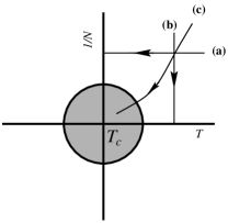
FIG. 1.: Schematic diagram showing the various paths in $T$ vs $N^{-1}$ plane, around the critical point $T=T_{c}$.

If we study the free energy, which cannot diverge, we might in principle write down an expansion of the type proposed in Eq. 14. This expansion is in $N$ for any $T$. From such a free-energy, we might compute the specific heat by taking derivatives and face again the problem of infinities on the right hand side at $T=T_{c}$. Another way of saying the same thing is that the free energy at the critical point behaves as $N^{1+q}$ with $q\leq 0$ but the specific heat obtained by taking derivatives of the free energy with respect to temperature gets a different power of $N$. This means that $N$ and temperature occur as a combination variable and not independently so that the limits $N\rightarrow\infty$ and $T\rightarrow T_{c}$ (taking derivatives) may not commute. The double limit needs to be considered carefully.

The dilemma is shown schematically in Fig. 1. The expansion in $N$, Eq. (14), is valid along path (a) ( $T\rightarrow T_{c}$ for a fixed $N<\infty$) and path (b) ( thermodynamic limit for a fixed $T$), but the expansion is not valid in the neighbourhood of the critical point. The non-extensive behaviour gets reflected if the critical point $(T=T_{c},N^{-1}=0)$ is reached via a suitable path like (c) whose form is obtained in the next section. An isolated critical point does affect its neighbourhood as in any problem of non-uniform convergence. The neighbouring region (shaded in Fig 1) is called critical region.

Question remains: Can the specific heat be divergent?

1 Comments

• If the specific heat has the anomalous behaviour at $T=T_{c}$, then the energy-density is also expected to have so. In general if the response function for a variable $<\Phi>$ has a singular behaviour, the variable itself will also be singular. In the next section we see how these are related.

• With Eq. (15)in hand, we need to redo the argument made in Sec II regarding fluctuation. This is done in Section  VIII.

• Question of divergence of specific heat: The answer is obviously “no” for a single particle system with a simple Hamiltonian (perfect gas, oscillator, two-level system ..). For a noninteracting collection of such simple systems, the free energy is always proportional to $N$ and no criticality may occur even in the limit $N\rightarrow\infty$. Interaction is needed and essential for criticality.

V Generalized Scaling

The simple scaling of Eq. 10 needs to be modified to allow for the apparent non-extensive behaviour at a critical point. To show this we work in the ensemble with $T$ as the variable (and all other parameters are kept fixed at their critical values). More variables will be taken up after that. We start with a generalization of scaling and show that it works. After working out a few consequences, we discuss the physical significance of the original scaling hypothesis.

A One variable: temperature

Let us define $t=(T-T_{c})/T_{c}$. Remember that this is an intensive variable and would not have required any scale factor on rescaling as per Eq. 7 or Ex. (10). In order not to clutter the equations with extra symbols, we consider a lattice problem for which $N$ and $V$ can be interchanged (e.g. the Ising model of Eq.  (36)). Defining $N=L^{d}$ with $L$ as a linear dimension of a $d$-dimensional cube, we take a way out as

$$F(t,L)=b^{-d+y_{f}}\ F(b^{-y_{t}}t,bL),\quad\quad({\rm generalized\ homogeneity}),$$ (16)

from which Eq. (7) or Eq. (10) can be recovered for $y_{f}=y_{t}=0$. We first show that this generalized homogeneous function works and then, look at its consequences. Physical significance is discussed after that.

Choosing $b=L^{-1}$,

$$F(t,L)=L^{d}L^{-y_{f}}\ {\cal F}\left(\frac{t}{L^{-y_{t}}}\right),\Longrightarrow\ {\sf f}(t,L)=b^{-y_{f}}\ {\sf f}(b^{-y_{t}}t,bL),$$ (17)

where ${\sf f}(t,L)\equiv{1\over N}F(t,L)$ is the free-energy per unit volume. We used ${\cal F}(x)=F(x,1)$. Finiteness of free-energy requires $y_{f}>0$.

For $t\not=0$, demand extensivity. To get a linear dependence of $F$ on $N$, we require ${\cal F}(x)\sim|x|^{q}$ such that $-y_{f}+qy_{t}=0$. This gives

$$f(t)\equiv\lim_{L\rightarrow\infty}{\sf f}(t,L)\sim|t|^{y_{f}/y_{t}},\quad{\rm or}\quad f(t)=b^{-y_{f}}f(b^{y_{t}}t).$$ (18)

Since the free energy per particle cannot be infinite even at $T_{c}$, we need $y_{f}>0$ and $y_{t}>0$. The last expression could also be written as $f(t)=b^{-y_{f}/y_{t}}f(bt)$ by redefining $b$.

If we are right at the critical point, the free energy density behaves as

$$f(t=0,L)\ \sim\ L^{-y_{f}},$$ (19)

the “nonextensive” feature we are looking for. The generalized homogeneous function works.

Exercise V.1

Why cannot we choose $F(T-T_{c},L)=b^{-d+y_{f}}F(T-T_{c},bL)$ as a simple generalization? Hint: non-extensive everywhere.

Exercise V.2

Is there any other generalization (other than Eq. 16 ) that could have been done?

1 Comments

A few things are to be noted in these manipulations.

• A singularity of the free energy in the thermodynamic limit is manifest in Eq. 18 and the singular behaviour is a power law in the deviation from the critical point. These powers are called exponents.

• We at the end recovered the much coveted extensivity, everywhere save the critical point, but at the cost of a scaling of the intensive variable.

• What we are focusing here is the singular part of the free-energy. There could ( and will) be an analytic piece that will not show any such anomalous scaling.

• With a positive $y_{t}$, we realize that the effective temperature is further away from the critical temperature as the size is increased, if we want to keep the free energy per particle ( or per unit volume) the same. This desire to keep the same free energy per unit volume is consistent with the content of Eq. (8).

• A more dramatic result is that an argument ${L/|t|^{-1/y_{t}}}$ can be thought of as a comparison of the length or size of the system with a characteristic scale $\xi$ of the system. This scale $\xi$ diverges when $t\rightarrow 0$ as $\xi\sim|t|^{-\nu}$ where $\nu=1/y_{t}$.

• A diverging length scale is the hallmark of a critical point and in fact a critical point or criticality is defined as a point with a diverging length scale.

• No, we have neither devised a way of bypassing the Legendre transformation problem nor ignored it. We chose the right ensemble (i.e. right thermodynamic potential) to do our analysis. It is conceptually helpful to use the ensemble that involves the intensive variables. For example, in first-order transitions (like, say, solid-liquid transition) there would be discontinuities in some extensive variables like the density, the energy density, the entropy ( latent heat) etc, but the intensive variables remain continuous. It is this fact that prompts one to use vertex functions in field theoretic analysis - but that’s beyond the scope of these notes.

• It still begs the question: What is this length $\xi$?

2 Specific heat: power laws and exponents

The specific heat is $c\sim\partial^{2}f/\partial t^{2}$. From Eq. (18), choosing $b=|t|^{-1}$, it follows that $c\approx f^{\prime\prime}(\pm 1)\ |t|^{-2+y_{f}/y_{t}}$, where prime denotes derivatives and $\pm$ stands for $t{>\atop<}0$. Note that the specific heat shows a power law singularity with an exponent

$$\alpha=2-\frac{y_{f}}{y_{t}},\quad{\rm defining}\ \alpha\ {\rm via}\ c\ \sim|t|^{-\alpha},\ {\rm or}\ \alpha=-\ \lim_{t\rightarrow 0}\frac{\log c}{\log|t|}.$$ (20)

The exponent for divergence of $c$ is same on both sides of the critical point at $t=0$, though the amplitudes $f^{\prime\prime}(\pm 1)$ need not be the same.

For $L<\infty$, the specific heat behaviour is

c(t,L)= L^α/ν  C(t L^1/ν), (21)

making the $L$-dependence explicit as required by Eq. (15). We leave it to the reader to establish the relationship between ${\cal C}$ of Eq. (21) and ${\cal F}$ of Eq. ( (17).

Exercise V.3

The two-dimensional ferromagnetic Ising model, Eq. (12), in zero field ($h=0$) has a logarithmic divergence of specific heat, $c\sim-\ln|t|$. How will the above formulation handle this? Note also that $\ln x=\lim_{n\rightarrow 0}(x^{n}-1)/n$.

3 On exponents: hyper-scaling

Since free energy and energy-density cannot diverge, we need to have $\alpha<1$. This puts a limit

$${y_{f}\over y_{t}}\geq\ 1\ {\rm or}\ \ y_{f}\geq y_{t}\ {\rm or}\ \nu\ \geq{1\over y_{f}}.$$ (22)

At the critical point $k_{B}T_{c}$ is the energy scale, and therefore $F/(L^{d}k_{B}T_{c})$ dimensionally behaves like inverse volume. In absence of any other scale, one might expect

$$\frac{F(t=0,L)}{k_{B}T_{c}N}\ \sim\ L^{-d},\quad\Longrightarrow\framebox{{\hbox{y_f=d}}}.$$ (23)

A similar argument for $L\rightarrow\infty$, and $t\not=0$, would then give, with $\xi$ as the important length-scale,

$${f\over k_{B}T_{c}}\ \sim\ \xi^{-d}\sim t^{+d\nu},\quad\Longrightarrow\framebox{{\hbox{2-\alpha= d \nu}}}.$$ (24)

This relation between $\alpha$ and $\nu$ involving $d$ is called hyper-scaling. Putting all together

$${f\over k_{B}T_{c}}=L^{-d}\,{\cal F}\left(\frac{t}{L^{-1/\nu}}\right).$$ (25)

In general

$$2-\alpha=y_{f}\,\nu$$ (26)

where $y_{f}$ could be different from $d$ if some other length-scale plays an important role at the critical point.

We did get the value of $y_{f}$ easily under certain conditions, but it is not possible to obtain $\nu$. Needless to say, with other variables, there will be more exponents. The values of these exponents are to be determined either from experiments or from statistical mechanical calculations with appropriate Hamiltonians.

Exercise V.4

If there is no singularity for a finite system, then how can there be a diverging length scale in say Eq. (25)? How to interpret this properly? Hint: asymptotic expansion (see Ex V.5 and Eq. 39).

Exercise V.5

A problem from school algebra: Consider the sum $S(x,N)=\sum_{n=0}^{n=N-1}x^{n}$ for $x\leq 1$. Show that for large $N$, and $x$ close to $1$, $S(x,N)=N\tilde{S}(Nt)$ where $t=1-x$, and $\tilde{S}(z)=(1-e^{-z})/z$. Recover, from this asymptotic form, the exact result (i) for $N\rightarrow\infty$ for any $x$ (Path b of Fig. 1), and (ii) for $x\rightarrow 1$ for any finite $N$ (Path a of Fig. 1). Compute numerically $S(x,N)$ for various values of $N$ and $x\leq 1$, plot $S(x,N)/N$ vs $Nt$ and compare with $\tilde{S}(z)$ (Path c of Fig. 1). Note the strong deviation from the asymptotic scaling for small $N$ or large deviation of $x$ from $1$. This is actually a comparison of the partial sums of the infinite series around the singular point.

4 Role of fluctuations: upper critical dimension: I

From the form of the free-energy, the finite-size scaling of the energy at $T=T_{c}$ can be obtained, namely $E/N\sim L^{-(1-\alpha)/\nu}$. Let us now go back to Eq. (6). The relative width of the distribution for $E$ is given by

$$\frac{\Delta E}{E}\sim L^{\alpha/2\nu}L^{(1-\alpha)/\nu}L^{-d/2}=L^{(y_{f}-d)/2},$$ (27)

remembering that $N=L^{d}$, and using Eq. (26). If now hyper-scaling is valid, $y_{f}=d$, and see, the relative width does not vanish even in the limit of $L\rightarrow\infty$. Therefore for such a case, fluctuation plays a crucial role. If, however, $y_{f}<d$, then the relative width vanishes in the thermodynamic limit. We then get a situation where we have a critical point with a diverging length-scale and possibly diverging response functions, but the effect of fluctuations is not strong in the sense that the probability distribution remains sharp around the average value. Similar results are found for other extensive variables also as shown in Sec V C 4.

One thing becomes clear: the dimensionality of the system is very important and the lower the dimensionality the stronger is the effect of fluctuations. We might expect that for large enough $d$, this condition $y_{f}<d$ will be satisfied. One may then try to understand such critical systems by considering the average system ignoring fluctuations altogether. This class of theories is called mean-field theory.

If there is a finite value of $d=d_{u}$ above which $y_{f}<d$, then fluctuations can be ignored for all $d>d_{u}$. This $d_{u}$ is called the upper critical dimension of the system. Hope would be that the effect of fluctuations can be studied in a controlled manner around this $d_{u}$ with $\epsilon=d_{u}-d$ as a small parameter. This is the basis of the $\epsilon$-expansion for many systems.

We, however, caution the reader that the finite-size scaling in a mean-field theory ( or $d>d_{u}$) is more complicated. We are concentrating only on the fluctuation dominated case.

B Solidarity with thermodynamics

The problem with extensivity can now be understood in terms of a diverging length scale. In the strict sense, there is actually no violation of extensivity. The idea of adding small pieces to build a bigger one makes sense provided the smaller pieces themselves are representative of the bulk. For systems with short range interactions and small intrinsic or characteristic length scales, this is reasonable because the “small size” effects or boundary effects are perceptible only if the size is comparable to these lengths. These effects are small corrections that can be safely ignored. In case of a diverging length-scale or characteristic length-scales larger than the system size, smaller pieces cannot be added up. Thus at a critical point with diverging length-scales, the notion of adding up smaller pieces fails. The length-scale $\xi$ is the appropriate scale for comparison and so at a critical point the whole sample is to be treated as a single one.

At any temperature $t\not=0$, $\xi\sim|t|^{-\nu}$ is large but finite. If we take a block of size $\xi^{d}$ as a unit, then extensivity requires that the free energy be proportional to the number of such blocks or blobs i.e. $F=(N/\xi^{d})\,f_{0}\sim N|t|^{d\nu}f_{0}$, with $f_{0}$ as the free-energy per blob. If $f_{0}$ is independent of $\xi$, then $f\sim f_{0}\,|t|^{d\nu}$, recovering Eq. (24). In case $f_{0}$, the free energy of a blob of volume $\xi^{d}$, depends on $\xi$, then extra $\xi$ contribution is expected and one gets Eq. (26) with $y_{f}\not=d$.

Exercise V.6

Anisotropic system: A particular two-dimensional system of size $L_{x}\times L_{y}$ shows the following scaling behaviour

$$f(t,L_{x},L_{y})\approx X{\sf f}\left(L_{x}t^{\nu_{x}},L_{y}t^{\nu_{y}}\right),$$ (28)

$X$ being the size dependent prefactor. There are now two different length scales in the two directions. What are the length-scale exponents? Find the relation (hyper-scaling) among $\alpha,\nu_{x}$ and $\nu_{y}$. What would be the form of $X$ if one takes $L_{x}\times\infty$ strips. (Ans: $X=L_{x}^{\alpha/\nu_{x}}$.)  What would be $X$ for $\infty\times L_{y}$ strips? We assume that the strips do not show any phase transition. What would be the right combination variable if both $L_{x}$ and $L_{y}$ are to be used in the prefactor? (Ans: $X=(L_{x}^{-1/\nu_{x}}+L_{y}^{-1/\nu_{y}})^{-\alpha}$. Why?)

Exercise V.7

Cross-over: Think of a cylindrical geometry. The system is finite in one direction (length $L$) but infinite in the remaining $d-1$ directions. There will be a critical behaviour in this geometry if $d$ is not too small. Consider the $d-1$ to $d$ dimensional crossover as the finite length $L$ is made larger. Consider various situations: (a) $d<d_{u}$, (b) $d>d_{u}$ but $d-1<d_{u}$, and (c) $d-1>d_{u}$.

C More Variables: temperature and field

Generalization of the scaling of Eq. (16) to more variables is straight forward. Take a variable $h$ which represents another intensive quantity like pressure, magnetic field etc, measured from its critical value. The critical point is now at $t=0,h=0$. The free energy can be written as

$$F(t,h,L)=b^{-d+y_{f}}\ F(b^{-y_{t}}t,b^{-y_{h}}h,bL),\quad{\buildrel N\rightarrow\infty\over{\Longrightarrow}}f(t,h)=b^{y_{f}}f(b^{-y_{t}}t,b^{-y_{h}}h),$$ (29)

so that the same series of manipulations done for $h=0$ would lead to

$${\sf f}(T,h,L)\equiv\frac{1}{N}F(t,h,L) = \xi^{-y_{f}}{\cal F}_{\pm}\left({h\over\xi^{-y_{h}}},{L\over\xi}\right),$$ (31)

$$= L^{-y_{f}}\tilde{\cal F}\left(\frac{t}{L^{-1/\nu}},\frac{h}{L^{-y_{h}}}\right),$$ (32)

where ${\cal F}_{\pm}(x,y)=F(\pm 1,x,y)$.

If $tL^{y_{t}}=const$, then, as per Eqs. (32) and (25), extensivity is nowhere to be found - that’s curve (c) in Fig 1. The scaling form of Eq. (25) or (32) is known as finite-size scaling.

1 Comments

• For a fixed $N$, if $t\rightarrow 0,$ then ${\sf f}\sim L^{-y_{f}}$.

• For a fixed $t$, if $N\rightarrow\infty,$ then

  $$f\sim|t|^{2-\alpha}\,\hat{\cal F}_{\pm}\left(\frac{h}{|t|^{y_{h}/y_{t}}}\right).$$ (33)

• We see the general feature:
  critical region $\Longleftrightarrow$  “nonextensivity”  $\Longleftrightarrow$  finite size scaling  $\Longleftrightarrow$  Scaling.

• Once we take the diverging length-scale as the sole scale for the problem, the finite-size scaling form can be obtained from the bulk behaviour as well. A finite length $L$ matters only when it is comparable to $\xi$. For $L\gg\xi$, the above-mentioned blob picture is valid and for $L<\xi$ the whole system needs to be treated as a critical one. If the bulk behaviour is like $c(t)\sim|t|^{-\alpha}$, then the size-dependent cross-over is given by ${\sf c}(t,L)\sim|t|^{-\alpha}\ \tilde{\cal C}(L/\xi,h/\xi^{y_{h}})$ $\sim L^{\alpha/\nu}\ {\cal C}(t/L^{-1/\nu},h/L^{y_{h}})$. (See Eq. (21).) Historically, bulk scaling was proposed first and finite-size scaling came later on.

• We cannot overemphasize the fact that $h$ and $t$ are completely independent variables. Yet in Eq. 33 the free-energy in the thermodynamic limit depends on the single combination variable $h/t^{y_{f}/y_{t}}$, and not on $h$ and $t$ separately. Results of experiments (real or numerical) done at various values of $h$ and $t$ can be collapsed on to a single curve, unthinkable away from the critical region.

• It seems there is one exponent too many for the bulk free energy density $f$ in Eq. (29), $y_{f}/y_{t}$ and $y_{h}/y_{t}$ would have sufficed. Yes, it would if we consider thermodynamics alone. But the path via finite-sized system showed us the necessity of another exponent, $\nu$, and so we keep all the three in Eq. (29).

Exercise V.8

Take the Legendre transform of $f$ in Eq. (29) with respect to $t$. Discuss its scaling property. Caution: The scaling is not for the total entropy or entropy density. The special scaling is for the deviation from the critical value of the entropy at the critical point. This shows the difference of the scaling around the critical point and the simple scaling of thermodynamics.

2 More variables mean more exponents

The power laws we saw earlier tend to suggest similar behaviour for other physical quantities also. We define several such practically important exponents, but shall ultimately see that all of these can be expressed in terms of the three $y_{f},y_{t},y_{h}$ introduced earlier.

For concreteness, the magnetic language of the Ising model of Eq. (12) is used. Let us assume that there is a critical point for the Ising model (and there is one) so that the free energy is given by Eq, ( 33). We have already defined $\alpha$ as the specific heat exponent. We define $\beta$ for magnetization, $\gamma$ for susceptibility, $\delta$ for critical isotherm. Apart from these thermodynamic exponents, two other expoents are needed $\nu$ ( already introduced) for length-scale and $\eta$ for critical correlations.

Remembering that the magnetization is the derivative of the free-energy with respect to $h$, one gets $m\approx|t|^{(y_{f}-y_{h})/y_{t}}{\cal F}_{\pm}\!^{\prime}(h/t^{y_{h}/y_{f}})$. From this, see that for $h=0$, the magnetization vanishes at the critical point as

$$m\sim|t|^{\beta},\quad{\rm with}\quad\beta=(y_{f}-y_{h})/y_{t}.$$ (34)

For a ferromagnetic transition, there is no magnetization in zero magnetic field in the high temperature phase (paramagnet), and therefore ${\cal F}_{+}\!^{\prime}(0)=0$ but ${\cal F}_{-}\!^{\prime}(0)\not=0$. A quantity like $m$ that describes the “ordering” of the system is called an order parameter and $\beta$ is the order-parameter exponent. We repeat that phase transitions need not necessarily have an order parameter (see Sec. VII B).

Susceptibility $\chi$ is the response of magnetization, and we see in zero field ( $h=0$) ($\chi=\partial m/\partial h$)

$$\chi\sim|t|^{-\gamma},\quad{\rm with}\quad\gamma=(2y_{h}-y_{f})/y_{t}.$$ (35)

At the critical point ($t=0$) in presence of a field ( critical isochore ), we get

$$m\approx h^{1/\delta}m_{0},\quad\delta={y_{h}/(y_{f}-y_{h})}.$$ (36)

Here the amplitude $m_{0}=\lim_{x\rightarrow\infty}x^{-(y_{f}-y_{h})/y_{h}}{\cal F}^{\prime}_{\pm}(x)$. In general, $\delta\not=1$. One expects a linear relationship (“linear response”) between “cause” ($h$) and “effect” ($m$), but that turns out not to be the case at criticality. A linear relation can never give an infinite $\chi$!

A major consequence of the homogeneity of the free energy is the power law behaviour of various physical quantities (various derivative of free energy) and all of these are obtained from the three basic exponents. In case of hyper-scaling (i.e. $y_{f}=d$) we have a further reduction and only two exponents are needed for a complete description of the critical behaviour of a system.

For a thermodynamic description this looks enough, but we already saw the usefulness of a length-scale based analysis. We need to define the length-scale properly and in the process we will find a more useful critical exponent $\eta$.

3 Comments

• The blob picture can be used for susceptibility near the critical point. There are $N/\xi^{d}$ blobs. Each blob of size $\xi^{d}$ can be thought of as a critical object. The total susceptibility is given by $N\chi=(N/\xi^{d})\chi_{\rm blob}$, where $\chi_{\rm blob}$ is the total susceptibility of a blob. Finite-size scaling predicts $\chi_{\rm blob}=\xi^{d}\xi^{\gamma/\nu}$ so that we obtain $\chi\sim|t|^{-\gamma}$

• Note that we require $y_{h}<y_{f}<2y_{h}$.

4 Role of fluctuations: upper critical dimension:II

The role of fluctuations was analyzed earlier in the context of specific heat. Let us now reanalyze it for the probability distribution for magnetization $M$. The finite-size scaling behaviours of (total) magnetization and (total) susceptibility at $T=T_{c}$ are $\langle M\rangle\sim L^{d}L^{-\beta/\nu}$ and $N\chi\sim L^{d}L^{\gamma/\nu}$. The relative width $\Delta M/M$ of the probability distribution for $M$ is $L^{\gamma/2\nu}L^{\beta/\nu}L^{-d/2}=L^{(y_{f}-d)/2}$ where Eqs. (37) and (26) have been used.

It is reassuring that the condition for sharpness (or broadness) of the probability distribution for $M$ is the same as obtained for specific heat (see Sec. V A 4). The upper critical dimension is the same no matter which conjugate pair we use.

D On exponent relations

Once the exponent identifications are made, with only two independent ones, it is possible to write down many relations involving the (in principle) experimentally measurable exponents. For example, by adding the exponents,

$$\alpha+2\beta+\gamma=2.$$ (37)

If we take the free-energy density $\sim hm$ and $m=\chi^{-1}h$, then it follows that $2\beta+\gamma=2-\alpha$, as in the above equation, without using any explicit formula. Another way of re-writing the above relation $(-\alpha=2(\beta-1)-\gamma)$ suggests that the behaviour of specific heat ($c_{h=0}$) is similar to $(\partial m/\partial t)^{2}\chi^{-1}$. In fact, thermodynamics gives us the formula

$$c_{h}-c_{m}=T\left(\frac{\partial m}{\partial T}\right)_{h}^{2}\chi_{T}^{-1},$$ (38)

where $c_{x}$ is the specific heat with $x$ constant. Since specific heat is positive definite, it follows from Eq. (38) for $c_{h}$ with the intensive variable $h$ held constant at the critical value $h=0$ that $\alpha+2\beta+\gamma\geq 2$.

Exercise V.9

Thermodynamic argument seems to indicate inequality rather than equality in Eq. (37). Find out the conditions for which a strict inequality is expected.

VI Relevance, irrelevance and Universality

A few observations should not miss our attention. Since $y_{t}>0$, the combination variable $Lt^{1/y_{t}}$ in, say, Eq. (21) or (32) have different limits for $t=0$ and $t\not=0$ in the limit $L\rightarrow\infty$. This difference actually gave us the different $L$-dependent behaviour of the free-energy or the specific heat, or, as a matter of fact, any physical quantity we may calculate or observe. In the same way, if $y_{h}>0$, then in the bulk case, if $t\rightarrow 0$, i.e. as the critical point is approached, the combination or scaling variable $h/t^{y_{h}/y_{t}}$ goes on increasing if $h\not=0$, no matter how small it is. The behaviour is different if $h$ is strictly zero. Such a tendency of a parameter to grow also tells us that zero field and nonzero field behaviours are different. We call these variables relevant variables.

In case $y_{h}<0$, then for $t\rightarrow 0$, the scaled variable is zero irrespective of its value. In such a case whether the system has $h\not=0$ to start with is immaterial. No wonder these are to be called irrelevant variables.

There could also be redundant terms that don’t matter at all, like a constant added to a Hamiltonian. We ignore them altogether.

To be at a critical point, the relevant variables must be tuned properly to be at their critical values (e.g. $t=h=0$ in the magnetic example) because they take us away from the critical point. Irrelevant variables don’t matter as such but they do play a significant role if we want to go beyond the leading behaviour.

Special situations arise, if the scaled function shows a singularity as an irrelevant variable scales to zero. Such variables are then important for the critical behaviour, though they don’t take the system away from criticality. Such a variable is called a dangerous irrelevant variable.

Critical points are classified by the number of relevant variables required to describe them. An ordinary critical point requires two (for the magnetic problem temperature and magnetic field, for the liquid-gas transition temperature and pressure). If three relevant parameters are needed it is called a tricritical point and so on.

Our analysis so far has been restricted to thermodynamic parameters like $t,h$ etc, but this can be extended to any parameter occurring in the Hamiltonian in a statistical mechanical approach. The starting Hamiltonian may have a large number of parameters based on the microscopic details of the system. But as we look at longer length-scales close to the critical point, all these parameters can be classified under the banner of relevance and irrelevance. By throwing away the irrelevant terms, for the leading behaviour, an enormous simplification ensues (e.g, all ordinary critical points will have only two relevant parameters, only difference may be in the numerical values of the exponents $\nu$ and $\eta$, etc.). It might then be expected that the numerical values of the exponents could be identified from certain basic symmetries etc of the Hamiltonian. This is the concept of Universality. A universality class would be described by the exponents and also the amplitude ratios of the various singular quantities on the both sides of the critical point.

The idea of universality transcends the domain of critical phenomena. Whenever we are interested in properties on a scale much bigger than the underlying or microscopic scales, there seems to be a set of properties which are quantitatively same no matter what the microscopic details are. The exponents we have seen are just one such examples. Historically it was found that the shape of the coexistence curve near the liquid-vapour critical point is independent of the chemical composition and is also very similar to the critical behaviour of several magnets. Once the universality class of a system is identified, the set of universal quantities can be obtained by studying a simpler model system than the original one with all details. The simpler model is expected to focus on the relevant variables only or at most a few irrelevant ones.

Universality is not just a set of exponents. In a scaling description, the amplitudes and even the scaling functions are independent of gross details except that the arguments of the functions may involve nonuniversal metric factors. In a finite size scaling there could be a dependence on the boundary conditions as well.

Whether a variable is relevant or not is determined by its scaling exponent (e.g. $y_{h}$ in the previous case). In certain cases, one may get these by simple arguments (Gaussian model in Sec. IX) but in most cases these are to be determined.

Exercise VI.1

Can there be critical cases with only one relevant variable or no relevant variables at all?

VII Digression: first-order transition and transition with no ordering

A A first-order transition: $\alpha$=1

What happens at the borderline of $\alpha=1$? The form of the free-energy tells us that the energy-density will have a discontinuity on the two sides of the singular point. Such a phase transition with a discontinuity in any first derivative of the free-energy is defined as a first-order transition. This value of $\alpha$ leads to $\nu=1/d$.

We see the possibility of a first order transition in the same framework developed for the critical point. But first-order transitions can be of other types also, and they may not necessarily have any diverging length-scales associated with it. One needs to be careful about it.

As an example, let us consider a very simple configuration space for a magnet (a crude approximation to an Ising-type model). We replace the $N$-spin configurations by two types only. A zero-energy ground state – all spins up or all down – two-fold degenerate, and an excited state of energy $N\epsilon$ with degeneracy $2^{N}$. (This is a one-dimensional ferro-electric six vertex model, in disguise.) The partition function for this model is $Z(x,N)=2+(2x)^{N}$ where $x=\exp(-\beta\epsilon)$. It is easy to see, by taking the $N\rightarrow\infty$ limit, that there is first-order transition at $x=1/2$ with total energy going from zero for $x<1/2$ to $N\epsilon$ for $x>1/2$. No problem with extensivity for $x\neq 1/2$. In the limit $N\rightarrow\infty$, the specific heat is just a delta function at the transition point. For finite $N$, the specific heat can be written in the form

$$C(x,N)=N^{2}\ \ln 2\ \frac{2e^{Nt}}{(2+e^{Nt})^{2}},$$ (39)

where $t=1-2x$. For a $d$-dimensional system, take $N=L^{d}$. What we now see from the scaling variable that there is a diverging length scale with exponent $\nu=1/d$.

1 Comments

• Fig 2 shows $C(x,N)$ for various values of $x$ and $N$ computed from the partition function and compared with the scaling function of Eq. 39. This is an example of data collapse.

• The thermodynamic limit for any given value of $x$ (Path b of Fig. 1) comes from the tail of the scaling function of Fig 2. This plot amplifies the critical region of Fig. 1.

• The $N^{2}$ prefactor in Eq. 39 is consistent with an exponent $\alpha/\nu$ with $\alpha=1$. Remember that $N=L^{d}$.

• The peak of the scaling function in Fig. 2 is not at the bulk transition point.

  Exercise VII.1

  What is this length scale in the context of this model?

  

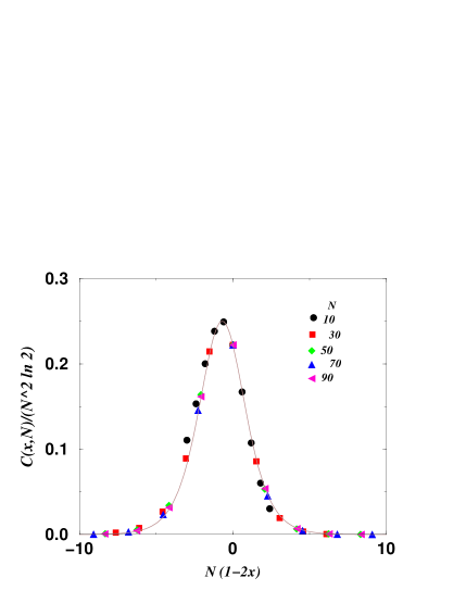
  FIG. 2.: Data collapse of $C(x,N)/N^{2}$ vs $Nt$ for various $N$. The solid line is the finite-size scaling function of Eq. 39.

This simple model calculation can be generalized. One way of studying a first-order transition is to compute the free energies of the two phases independently ( like e.g. solid and liquid) and then finding the lower free energy curve. Taking these free energies per particle, $f_{1}$ and $f_{2}$, as coming from a restricted sum over states of the full partition function, the total partition function can be approximated by $Z=\exp(-N\beta f_{1})+\exp(-N\beta f_{2})$, with the free energy per particle $f=\min(f_{1},f_{2})$ for $N\rightarrow\infty$. In general, $f_{i}$’s are analytic function and the transition temperature is determined by $f_{1}(T_{c})=f_{2}(T_{c})$, so that $\Delta f=|f_{1}(T)-f_{2}(T)|\sim|T-T_{c}|$ from a Taylor series expansion around $T=T_{c}$. The partition function can therefore be written as $Z=\exp(-N\beta f)\ [1+\exp(-N/\xi^{d})]$, where $\xi^{-d}=\beta_{c}|\Delta f|$. This defines a length scale $\xi\sim|T-T_{c}|^{-1/d}$. For first-order transitions, $\nu=1/d$.

B Example: Polymers : no “ordering”

We give an example here of a phase transition for which there is no “ordering” unlike the magnetic case, and the interest in the critical point is because of finite-size behaviour.

Polymers are long linear objects, abundantly occurring in nature. Let us take a single flexible polymer in a solvent ( a single polymer of length $N$ in $d$-dimensional space of infinite volume). Depending on the nature of the solvent and the monomers constituting the polymer, there could be effective repulsion or attraction between the monomers. By changing temperature, one may go from a repulsion-dominated (monomer favouring solvent molecules) (self avoiding walk) to an attraction-dominated (monomer preferring monomer) phase. This is called a collapse transition. Such a transition for a single molecule can occur only in the thermodynamic limit of length $N\rightarrow\infty$. But that’s of no interest because the polymers are necessarily of finite lengths. The two phases in this example are described by the overall size of the polymer, e.g. by the mean square end-to-end distance $\langle R^{2}\rangle\sim N^{2\nu}$. In a collapse transition the value of this size exponent $\nu$ changes from $\nu\approx 3/(d+2)$ to $\nu=1/d$ in $d$-dimensions. This is an example of a phase transition or critical point which may not be viewed as ordering (unlike the magnetic system) - no less important though. The main features of the transition are reflected in the “finite-size” behaviour (with respect to $N$) both at the transition and in the two phases, and the general analysis we have done so far is easily applicable here.

Exercise VII.2

What sort of a critical point is the collapse transition? Hint: How many relevant parameters at a collapse transition? We need to make length going to infinity, we need to adjust temperature and if we take a solution of polymers, we need to make concentration equal to zero ( i.e. single chain limit).
Ans: tricritical point.

Exercise VII.3

For a polymeric phase transition of the type mentioned above, show that the specific heat per unit length (or per monomer) can be written in a scaling form $c=N^{2\phi-1}{\cal C}((T-T_{c})N^{\phi})$

VIII Exponents and correlations

A Correlation function

Consider the Ising model of Eq. (12) or  (13) and take $M=\sum_{i}\langle s_{i}\rangle$. The fluctuation-response theorem of Eq. (11) and translational invariance can be used to express the susceptibility ($\chi$ per particle) as

$$\framebox{{\hbox{N\chi= (k_BT)^{-1} \sum_i\sum_j \langle(s_i - \langle s\rangle) (s_j - \langle s\rangle) \rangle= N(k_BT)^{-1} \sum_{\vec{x}} g({\vec{x}})}}},$$ (40)

where $g(\vec{x})$ = $\langle(s_{0}-\langle s\rangle)(s_{\vec{x}}-\langle s\rangle)\rangle$ is the pair correlation function. The behaviour of the susceptibility is therefore dependent on the behaviour of the correlation function. This relation is quite general as pointed out in section III B 1. By expressing the total quantity $\Phi=\sum_{\bf x}\phi({\bf x})$, in terms of a local density, we have $\langle\Phi^{2}\rangle-\langle\Phi\rangle^{2}$ $=N\sum_{\bf x}g_{\phi\phi}({\bf x})$, where $g_{\phi\phi}({\bf x})=$ $\langle(\phi(0)-\langle\phi\rangle)(\phi({\bf x})-\langle\phi\rangle)\rangle$.

For simplicity, let’s replace the sum in Eq. (40) by an integral so that $\chi=\int d^{d}xg(\vec{x})$. For the Ising case, $s$ is bounded and so is $g$. We also know that $\chi$ diverges at least at $T_{c}$. Only way this can happen is from the divergence of the integral or the sum - it is the large distance property of $g(x)$ that controls the behaviour. We can conclude that, at least at $T_{c}$, $g(x)$ cannot be a short ranged function, but it has to decay to zero for infinitely large distances. In $d$ dimensions, the decay at $T=T_{c}$ for large $x$ is given by

$$\framebox{{\hbox{g(\vec{x}) \sim x^{-(d-2+\eta)}}}}\quad{\rm with}\quad\eta\geq 0\quad\quad(T=T_{c}).$$ (41)

For $T\neq T_{c}$, convergence requires that $g(r)$ should decay sufficiently faster than this, better be of short-range character with a characteristic length scale $\xi$, e.g. $\exp(-x/\xi)$. The decay for any temperature can be written as

$$g(\vec{x})=\frac{1}{x^{d-2+\eta}}\ {\sf g}\left(\frac{x}{\xi}\right)\quad\quad(T\not=T_{c}),\quad\quad{\rm(see\ comments\ below)}$$ (42)

which goes over to the $T=T_{c}$ case if this length-scale $\xi$ diverges for $T\rightarrow T_{c}$. The length-scale we saw popping out naturally for comparisons of the length of the system can now be identified as the correlation length, the scale for correlations. A precise definition of $\xi$ would be from the second moment of $g({\vec{x}})$ as

$$\xi^{2}=\frac{\int d^{d}{x}\ x^{2}g({\vec{x}})}{\int d^{d}{x}\ g({\vec{x}})}\sim|t|^{-2\nu}.$$ (43)

(For an isotropic system, the first moment vanishes by symmetry.) It is possible to define such scales via higher moments also. Under the assumption of one scale, all of these will have similar divergences at a critical point. Nevertheless, it is worth keeping in mind that there are cases where one may need to study higher order moments and different moments defining different length-scales.

Exercise VIII.1

Can $\eta<0$?

Exercise VIII.2

Generalize Eq. (43) for anisotropic cases like in Ex. V.7.

1 Comments

• The on-site term, $i=j$, with prefactor $(k_{B}T)^{-1}$ in Eq. 40 is the susceptibility of individual spins (or isolated degree of freedom), the Curie susceptibility. The correlation contribution is special to an interacting system. Note that the correlation vanishes for a noninteracting system.

• The fluctuation becomes long-ranged at the critical point. On the high temperature side $\langle s_{i}\rangle=0$ ( no magnetization), and so the fluctuation correlation is the same as the spin-spin correlation.

• For low temperatures ($T<T_{c}$), the spin-spin correlation approaches a constant ($\langle s\rangle^{2}\neq 0$) for large separations. This approach to the constant value is generally short-ranged, i.e., very rapid like exponential but becomes long-ranged at $T_{c}$.

• We get a long-range correlation even though the interactions are just short ranged ( e.g., nearest neighbour interaction in the chosen Ising model).

• A finite size scaling for the correlation length itself would be $\xi\sim L$. Quite often it is possible to write it as an equality with the amplitude determined by the known exponents. The amplitude surely depends on which correlation function is used to determine $\xi$, boundary conditions etc.

• For historical reasons Eq. (42) is generally written in a slightly different form as $g(\vec{x})=\frac{1}{x^{d-2+\eta}}\ {\sf D}\left(\frac{x}{\xi}\right)\exp(-x/\xi)$, with $D(z)\rightarrow 1$ for $z\rightarrow 0$, while $D(z)\sim z^{(d-3+2\eta)/2}$ for large $z$. Such a form is required to make correspondence with the Ornstein-Zernicke theory of correlations, which we shall not discuss in these notes.

B Relations among the exponents

Let’s think of the pair correlation function. It decays rapidly once we are on a scale greater than the correlation length $\xi$. Close to $T_{c}$, we can think of the system as blobs of highly correlated regions - the blobs are of size $\xi^{d}$ in $d$ dimensions. These are the blobs we introduced to salvage extensivity in Sec. V B. Inside a blob $(r<<\xi)$, the fluctuations are critical-like and at a simple level, a blob can be thought of as at $T_{c}$. On a bigger length scale $x>>\xi$, the blobs are independent. Basically, we are arguing that it is the correlation length that matters - all other length scales are unimportant.

We use this simple picture for the susceptibility. We can cutoff the integral at $x\sim\xi$, and inside this region $g(x)\sim x^{-(d-2+\eta)}$. The integral $\int^{\xi}dx\ x^{1-\eta}\sim\xi^{2-\eta}$. Using the temperature dependence of $\xi$, we get the temperature dependence of $\chi$ as $\mid t\mid^{-\nu(2-\eta)}$. The net result is

$$\gamma=\nu(2-\eta).$$ (44)

This relation with the help of Eq. (35) gives

$$y_{h}=\frac{y_{f}+2-\eta}{2}.$$ (45)

This is a very important relation - it shows how the external magnetic field or the nonthermal relevant variable scales away from the critical point is determined by the decay of correlations at criticality.

It is straightforward to see that $\alpha=\nu(2-\eta_{E})$.

C And it’s correlations

We now have the full identification of the three exponents:

$$\framebox{{\hbox{y_t=1/\nu, \ y_f= d, \ y_h=\frac{d+2 -\eta}{2}}}}.$$ (46)

All the nuances of critical phenomena are qualitatively and quantitatively expressed in terms of the correlation function and the exponents needed for it. It’s a shift from a thermodynamic description to a purely statistical mechanical one. It is the correlations of the degrees of freedom that control completely the whole phenomenon.

In this particular example of ordinary critical point, one of the exponents, $\eta$ is really an exponent defined at criticality, while the other,$\nu$, is an off-critical one. An off-critical exponent helps in the description of the approach to the criticality. This can however be treaded for purely critical exponents.

Exercise VIII.3

What if $y_{f}\not=d$?

1 Comments

• Now that we have emphasized the role of correlation functions and expressed $y_{h}$ in terms of $\eta$, why are we not doing the same thing for specific heat? Eq. (6) tells us that specific heat is related to energy-energy correlation function, and so shouldn’t we define an exponent $\eta_{\rm E}$? We could if we want to. But convince yourself, by using hyper-scaling, that $y_{t}=1/\nu=(d+2-\eta_{\rm E})/2$. We may use either $\nu$ or $\eta_{\rm E}$.

• One may generalize the analysis of Sec.VIII A for any local variable $L(\{\phi(x)\})$ and the corresponding response function will be determined by the critical correlation of $\langle L(\{\phi(x_{1})\})L(\{\phi(x_{2})\})\rangle$.

In a correlation based approach, we need to compute the critical correlations of all possible combinations of the degrees of freedom (e.g. in the Ising case, spin-spin, energy-energy and so on). From these, the relevant variables can be identified. In the Ising criticality case, there are only two. In addition, for a thermodynamic problem, we need to know the finite size behaviour of the free energy at the critical point (or assume hyperscaling). These three critical parameters then completely specify the leading behaviour even around the transition point.

To repeat, a thermodynamic description would focus on $y_{f},y_{t},y_{h}$ for a critical point, while statistical mechanical description would focus on the set of purely critical exponents $y_{f}/y_{t},\eta_{\rm E}$, and $\eta$. The scaling relations we derived show their equivalence.

Exercise VIII.4

Can this happen: the spin-spin correlation function is given by Eq. (42) and the energy-energy correlation is given by $g_{EE}\sim x^{-(d-2+\eta_{E})}{\sf g}_{E}(x/\xi_{E})$ where $\xi_{E}\sim|t|^{-\nu_{E}}$, but $\nu_{E}\not=\nu$?

D What’s $b$ anyway? : length-scale dependent parameters

If we look at the free energy of Eq. (18) or Eq. (29) in the thermodynamic limit of $L\rightarrow\infty$, a question may be asked, “what is $b$ now?”. Answer is in the correlation function. Under a rescaling $x\rightarrow x/b$, we see $g(x,t)=b^{-(d-2+\eta)}g(x/b,b^{y_{t}}t)$, where the $t$-dependence has been made explicit. This resembles the scaling of the free-energy. An interpretation of this equation is that if we change the scale of length measurements (actually the scale of microscopic details - though not apparent right now), the parameters of the problem and the concerned physical quantity get rescaled. Quantitatively, for $x\rightarrow x^{\prime}=x/b$, we have $t\rightarrow t^{\prime}=b^{y_{t}}t$, $h\rightarrow h^{\prime}=b^{y_{h}}h$, and $f\rightarrow f^{\prime}=b^{y_{f}}f$.

For a given problem (i.e. $t,h,..$ fixed) such a scale transformation leads to a transformation of the parameters and the physical quantities. Repeated applications of this transformation would land us on a set of parameters which are functions of $b$. These are the scale dependent parameters - criticality is best understood in terms of these scale-dependent parameters.

The scale-dependence of the parameters is best represented by infinitesimal scale transformation $b=1+\delta l$ (compare with Ex. III.3). We may write down a differential equation for Eq. (18) as

$$\left(\zeta(t)\ \frac{\partial\ }{\partial t}-y_{f}\right)\ f=0,$$ (47)

where $\zeta(t)={\partial t}/{\partial l}=y_{t}t$. This equation has the expected solution $f\sim t^{y_{f}/y_{t}}$.

This is a new way of looking at the problem. Instead of studying a system for various values of the parameters ( “coupling constants”), we are studying it at various scales to see how it behaves in the long-scale limit, after all thermodynamic or macroscopic behaviour is for a large system.

The equation derived just above, (Eq. (47), describes the flow of the free-energy as the scale is changed, and such equations are called flow equations. Any physical quantity will have a flow equation associated with it. However with only a few relevant parameters and a few independent exponents, not all flow equations are necessary. A fuller picture emerges from a renormalization group analysis. Actual flow equations turn out to be slightly more complicated and the simpler equation of Eq. (47) is obtained under special conditions of “fixed points”. The critical behaviour and the universality classes are ultimately linked to the fixed points.

Exercise VIII.5

Possibility of a dangerous fixed point?: A fixed point by definition is a point that does not change under rescaling. If a parameter say $u$ has a stable fixed point at $u=u^{*}$ then $u-u^{*}$ can be taken as an irrelevant variable. Can this variable be a “dangerous irrelevant variable”, or, in other words, can there be a dangerous fixed point?

IX Models as examples: Gaussian and $\phi^{4}$

At this point it is helpful to consider a few examples. The Ising model has been introduced in Ex. III.6. Here we consider a continuum version of it. A naive continuum limit would give a Gaussian model for a field variable $-\infty<\phi<\infty$,

$$\frac{H}{k_{B}T}=\int d^{d}x\ [\frac{1}{2}(\nabla\phi)^{2}+\frac{1}{2}r\phi^{2}-h\phi]=\int\frac{d^{d}q}{(2\pi)^{d}}[\frac{1}{2}(q^{2}+r)\phi_{k}\phi_{-k}]-h\phi_{k=0},$$ (48)

with a cut-off in real space, i.e. $|x|>a$ or in momentum space $|q|<\Lambda\sim a^{-1}$, where $a$ could be the lattice spacing. We shall assume a spherical Brillouin zone. A better continuum limit is the $\phi^{4}$ model,

$$\frac{H}{k_{B}T}=\int d^{d}x\ [\frac{1}{2}(\nabla\phi)^{2}+\frac{1}{2}r\phi^{2}+u\phi^{4}].$$ (49)

Exercise IX.1

Starting from the Ising model on a hyper-cubic lattice of coordination number $q=2d$, get the continuum form given above. Show that $r\sim T-T_{m}$ with $T_{m}=qJ$.

The reason for considering a continuum limit is to take advantage of dimensional analysis. Both sides of Eqs. 48 and 49 being dimensionless and the right hand side expressed as a volume integral helps us in introducing a length based analysis in a natural way.

That $r=0$ is a singularity is obvious from Eq. (48) because of the instability at $r<0$. One can derive all the thermodynamic properties for the Gaussian model and convince oneself that there is a singularity at $r=0$. We do not go into that. Here let us accept that $r=0$ corresponds to a critical point.

• In general, one would have a term of the type $\frac{1}{2}c(\nabla\phi)^{2}$ in Eqs. 48 and 49. However, if $c$ does not change sign, one may absorb it in the definition of $\phi$ and redefine $r$ and $u$. This has been done in those two equations. There are problems where $c$ may change sign when external parameters are changed (Lifshitz point), and in such cases $c$ needs to be kept explicitly. It would be necessary to keep $c$ explicitly in case the field variable cannot be scaled arbitrarily, as e.g. if $\phi$ is like an angular variable.

A Specific heat for the Gaussian model

Using Gaussian integrations, one can compute the zero-field specific heat for the Gaussian model. The leading term is given by the integral

$$c_{h=0}\approx\xi^{4-d}\frac{Ta_{2}}{2}\ \frac{K_{d}}{(2\pi)^{d}}\,\int_{0}^{\Lambda\xi}\frac{q^{d-1}}{(1+q^{2})^{2}}\,dq+...,$$ (50)

where $\xi=r^{-1/2}$, $r=a_{2}(T-T_{m})$ and $K_{d}$ is the surface integral of a $d-$dimensional unit sphere. The length-scale exponent is $\nu=1/2$.

Exercise IX.2

Derive Eq. (50). Show that $\eta_{E}=d-2$.

A dimensional analysis gives

$$[\phi(x)]=L^{(2-d)/2},\ [r]=L^{-2},\ [\Lambda]=L^{-1},{\rm and}\ [u]=L^{d-4},[h]=L^{-(2+d)/2}.$$ (51)

where $L$ is a length scale. This simple dimensional analysis already identifies a diverging length-scale $\xi=r^{-1/2}$, used in Eq. (50). Note also that the specific heat is a volume integral of the $\phi^{2}$-$\phi^{2}$ correlation function in real space. A dimensionally correct form is therefore

$$c=\xi^{4-d}\ {\cal C}(u\xi^{4-d},h\xi^{(2+d)/2},\Lambda\xi).$$ (52)

We take the Gaussian model first ($u=0$) and no external field, $h=0$. Then $c=\xi^{4-d}{\cal C}(\Lambda\xi)$ and Eq. 50 is in this form. Take the limit $\xi\rightarrow\infty$. The behaviour of the specific heat now depends on ${\cal C}(z)$ as $z\rightarrow\infty$. If this limit is finite, then the cut-off can be completely forgotten and $\xi$ plays the important role. In such a case the microscopic parameters are not important for the critical behaviour. This happens, as we see from the integral in Eq. (50) for $d<4$, and $\alpha=(4-d)/2$, a value that satisfies hyper-scaling with $\nu=1/2$. However for $d>4$, the integral diverges at the upper limit and ${\cal C}(z)\sim z^{d-4}$, leaving us with a non-divergent specific heat, i.e. $\alpha=0$. Hyper-scaling also gets violated. For $h\not=0$, Gaussian integrations yield $y_{h}=(d+2)/2$, consistent with dimensional analysis. The exponents are

$$\framebox{{\hbox{y_f=d}} for {\hbox{d<4}}, but {\hbox{y_f=4}} for {\hbox{ d>4}}}\quad{\rm and}\quad\framebox{{\hbox{\nu=1/2}} and {\hbox{\eta=0}}, for all {\hbox{d}}}.$$ (53)

In the above example we chose the specific heat because of its interesting behaviour for $d<4$ and $d>4$. Take Susceptibility. Dimensional analysis gives $\chi\sim r^{-1}$. Convince yourself, by using Gaussian integrals, that this is so for all $d$. However the finite-size scaling behaviour will be different for $d<4$ and $d>4$.

From the value of $\alpha$ or $y_{f}$, (see Eq. 53) and the sharpness criterion of Sec. V A 4, we see that fluctuations can be ignored if $d>4$. In a sense $d=4$ turns out to be the upper-critical dimension for this model.

Exercise IX.3

Calculate the average energy of a Gaussian correlated blob. i.e. a blob of size $\xi^{d}$ - do this by calculating the form of the energy for the Gaussian model and then putting $r=0$. Study its behaviour for various $d$ and then integrating once with respect to $r$ estimate the free-energy $f_{0}$ of a blob (See Sec. V B). Justify the violation of hyper-scaling for $d>4$.

B Cut-off and anomalous dimensions

The above warm-up exercise shows that the cutoff, a relic of the microscopic features of the model, cannot always be ignored even-though the relevant length-scales at which the phenomenon is taking place is much much larger than this. Dimensionality is also important. Dimensional analysis is not expected to yield any unique or useful relation if there are multiple scales in the problem. This is a very important point and we elaborate on this further. In case the cutoff can be ignored, the exponents are the same as predicted by dimensional analysis. This we see directly in the Gaussian model for $d<4$ - the cut-off just didn’t matter.

Exercise IX.4

Consider a finite Gaussian model with periodic boundary conditions in all directions. Obtain the finite-size scaling behaviour of the specific heat for various $d$. Note the discrete $k$ sums with no $k=0$ mode.

Exercise IX.5

Do the finite-size scaling analysis for the zero-field susceptibility of the Gaussian model for various $d$.

If we go back to the $\phi^{4}$ problem, then we need to treat Eq. 52. Question now is what happens for $\xi\rightarrow\infty$. If ${\cal C}$ goes to a constant, this cutoff can be safely ignored. A general situation would be

$${\cal C}(x,y,z)=z^{p}\tilde{\cal C}(xz^{p_{1}},yz^{p_{2}}),\quad{\rm as}\ z\rightarrow\infty.$$ (54)

Setting $\Lambda=1$,

$$c\sim\xi^{(4-d)+p}\tilde{\cal C}(u\xi^{(d-4)+p_{1}},h\xi^{y_{h}+p_{2}}).$$ (55)

This has the expected scaling form when $\xi$ is replaced by $|t|^{-\nu}$. In fact the same analysis can be done for $\xi$ itself,

$$\xi=r^{-1/2}\ {\cal X}(ur^{(4-d)/2},...,\Lambda/\sqrt{r}),$$ (56)

and, in the $r\rightarrow 0$ limit, the rhs of Eq. 56 might (and would) pick up extra powers of $r$ from the $\Lambda$-dependent argument. This would then change the temperature dependent exponent of Eq. 55.

Seen from a thermodynamic point of view, these extra powers of $\xi$ are remarkable because these seem to vitiate dimensional analysis. An additional scale is needed, and this comes from the small length-scale $a\sim 1/\Lambda$ whenever there is fluctuations at all length scales. The ultimate exponent one observes are not what dimensional analysis based on $\xi$ as the important length-scale would have predicted, except for Gaussian-type models. (These dimensional-analysis-based exponents are called naive or engineering dimensions.) One needs to understand and explain the origin of the “extra” contribution like the $p$’s, which are to be called anomalous dimensions. Once the role of cut-off is recognized, the discrepancy with dimensional analysis (which is infallible in any case) vanishes.

Because of the long range nature of the correlations, any local fluctuation can affect regions away for it. This is the origin of scale-invariance or occurrence of power laws (scaling). However the occurrence of anomalous dimension is something more. In a Gaussian type model, the degrees of freedom can be decomposed into independent modes ( e.g. by going over to Fourier modes - “normal coordinates”) and then we see the emergence of long range correlation in the long distance limit of $q\rightarrow 0$. The modes remain independent so that the fluctuation at one scale determined by $q$ does not affect the fluctuations at other scales. For this reason dimensional analysis gives correct result. In contrast for a $\phi^{4}$ type model, the modes for different $q$-values are no longer independent (coupled by the $\phi^{4}$ term) and now a fluctuation at a short distance scale ( $q$ close to the cut-off) can affect the fluctuations at longer scales even to $q\rightarrow 0$.

The mode coupling allows a small fluctuation at some point in space to affect other points and the disturbance seen by any other point is the sum over all the paths that connect the two points in question. For low dimensions, this sum can have fluctuations and this leads to anomalous dimensions. In high enough dimensions, the availability of a large number of paths (phase space volume) helps in averaging out the effects. These two cases are separated by the upper critical dimension.

• Note that $u$ becomes irrelevant for $d>4$ and it could be a dangerous irrelevant variable. The exponents in such cases would depend on the function also.

C Through correlations

It is reasonable to expect that the scaling variable one sees in a given problem should be independent of the actual physical quantity one is looking at. Therefore in the limit of $\Lambda\rightarrow\infty$, anomalous dimension like $p_{2}$ for $h$ should be the same for all quantities that depend on $h$. Let us take the example of the correlation function, in zero field, at criticality,

$$g(x)=\frac{1}{x^{d-2}}{\sf g}(u\,x^{4-d},\Lambda x),$$ (57)

suppressing the arguments on the lhs. Now in the limit $\Lambda x\rightarrow\infty$, if ${\sf g}(...,z)=z^{-\eta}\tilde{\sf g}(....)$, where the nature of the other arguments are not so crucial for us right now, we have

$$g(x)=\frac{1}{x^{d-2+\eta}}\tilde{\sf g}(...)\quad({\rm setting}\ \Lambda=1).$$ (58)

This $\eta$ changes $y_{h}=(d+2)/2$ to $y_{h}=(d+2-\eta)/2$. Identification can therefore be made: $p_{2}=-\eta$.

Let us reanalyze the zero field critical correlation function $g(r,\Lambda)$, where the $\Lambda$-dependence has been made explicit. Under a rescaling of all lengths $x\rightarrow bx$, we see $g(x,t=0,\Lambda)=b^{-(d-2)}g(bx,0,\Lambda/b)$. The scale factor for the correlation function picks out the exponent one would expect on dimensional analysis. However if a scale transformation is done that changes the longer length-scales but not the microscopic ones, i.e. $\xi\rightarrow b\xi$ but $\Lambda\rightarrow\Lambda$, then

$$g(x,0,\Lambda)=b^{-(d-2+\eta)}g(bx,0,\Lambda)$$ (59)

In analogy with the naive dimension, we now define a scaling dimension which is the dimension one observes in the long scale limit keeping the microscopic lengths same.

Denoting the scaling dimension of $X$ by ${\cal S}_{X}$ from how $X$-$X$ correlation function scales as in Eq. (59), while naive dimension by $d_{X}$ ( defined by dimensional analysis), we have ${\cal S}_{\phi}=-(d-2+\eta)/2$ while $d_{\phi}=-(d-2)/2$. It is easy to check now that

$${\cal S}_{h}+{\cal S}_{\phi}=-d=d_{h}+d_{\phi}.$$ (60)

This relation for the every pair of conjugate variables is very useful. The scaling behaviour of say Eq. (55) can then be interpreted as dimensional analysis but with scaling dimensions. Renormalization group transformation is a way of doing a transformation that scales the long lengths keeping the short ones same, thereby picking the scaling dimensions.

Generalizing the above discussion, we may define the scaling dimension $S_{\psi}$ for any local quantity $\psi({\bf x})$ from the critical auto-correlation function, i.e. the long distance decay of the $\psi$-$\psi$ correlation. The analogue of dimensional analysis would tell us that for the critical correlation of any combination of local variables $\psi_{1},\psi_{2},...$, we should have

$$\langle\psi_{1}(0)\psi_{2}(x_{2})...\psi_{n}(x_{n})\rangle=|x_{2}|^{-S_{1}-S_{2}..-S_{n}}\ {\cal Y}\left(\frac{x_{3}}{x_{2}},...,\frac{x_{n}}{x_{2}}\right).$$ (61)

where $S_{i}$ is the scaling dimension of $\psi_{i}$.

Exercise IX.6

Why is it that the dimensions add up to $-d$? When can it be something different?

Exercise IX.7

Use dimensional analysis to write free-energy $f(r,u,h,\Lambda)$ and magnetization $m(r,u,h,\Lambda)$ as

$$f = \xi^{-d}\tilde{f}(u\xi^{4-d},h\xi^{(d+2)/2},\Lambda\xi),$$ (63)

$${\rm and}$$ (64)

$$m = \xi^{-(d-2)/2}\tilde{M}(u\xi^{4-d},h\xi^{(d+2)/2},\Lambda\xi),$$ (65)

where $\tilde{f},\tilde{M}$ are unspecified functions. For $\Lambda\xi\rightarrow\infty$ one expects anomalous dimensions:

$$f = \xi^{-d}\hat{f}(u\xi^{4-d+p_{u}},h\xi^{(d+2)/2+p_{h}}),$$ (66)

$${\rm and}$$ (67)

$$m = \xi^{-(d-2)/2+p_{m}}\hat{M}(u\xi^{4-d+p_{u}},h\xi^{(d+2)/2+p_{h}}).$$ (68)

Express these new functions in terms of the functions in Eqs. (63) and (65). Using the relation $m=\partial f/\partial h|_{h=0}$, show that $p_{m}=p_{h}\ \ (=-\eta)$.

X Conclusion

We attempted to give an introduction to critical phenomena especially the idea of scaling, its need and consequences. The emphasis is on diverging length-scales. In case of a diverging length scale, as at a critical point, the correlations become long ranged. Such a point is characterized by (i) the decay exponents of the correlations ( which could have anomalous part like $\eta$ and $\eta_{E}$ of Sec. VIII C), and (ii) the number and nature of the relevant variables at that point.

Any problem that does not have any intrinsic or important length-scale would behave like a critical system. This absence of length-scales leads to power law decays of correlations and also power laws for other physical quantities. In low dimensions ( less than the upper-critical dimension, which could very well be infinite) fluctuations play an important role near or at the critical point and show up in the anomalous exponents. In such cases (i.e. $d<d_{u}$), the finite-size effects can be understood in terms of the finite-size scaling.

Distinction needs to be made between scaling and anomalous dimension. Scaling is the rule for criticality, originating from a diverging length scale, while anomalous dimension is seen for fluctuation dominated cases.

Renormalization group provides the proper framework for analyzing such phenomena. We feel it is worthwhile to motivate those ideas behind RG at the introductory level. Mean-field theory that ignores fluctuations could then be placed in the proper perspective as special (called dangerous) behaviour of certain irrelevant variables.

- [1] A few references:
- [2] *** From 90’s:
- [3] S. M. Bhattacharjee, “Mean field theories” in Models and Techniques of Statistical Physics, (Narosa, New Delhi, 1997).
- [4] H. E. Stanley Scaling, universality, and renormalization: Three pillars of modern critical phenomena, Rev. Mod. Phys. 71, S358 (1999)
- [5] M. E. Fisher, Renormalization group theory: Its basis and formulation in statistical physics, Rev. Mod. Phys. 70, 2 (1998).
- [6] J. Cardy, Scaling and Renormalization in Statistical Physics (Cambridge U Press, 1996)
- [7] J. Zinn-Justin, Quantum field theory and critical phenomena, 3rd ed (Oxford, 1996).
- [8] C. Domb, The critical point: a historical introduction to the modern theory of critical phenomena (Taylor and Francis, 1996)
- [9] P. M. Chaikin and T. C. Lubensky, Principles of Condensed Matter Physics (Cambridge U Press, 1995).
- [10] S. V. G. Menon, Renormaliazation group theory of critical phenomena (Wiley Eastern, 1995).
- [11] J. Yeomans, Statistical Mechanics of phase transitions, (Oxford U. Press, 1992)
- [12] J. J. Binney, N. J. Dowrick, A. J. Fisher and M. E. J. Newman, The modern theory of critical phenomena, (Clarendon Press, 1992) *** From 80’s:
- [13] G. Parisi, statistical field theory (Addison-Wesley, 1988)
- [14] D. J. Amit, Field theory, the renormalization group, and critical phenomena, 2nd ed. (World Scientific, 1984)
- [15] R. J. Baxter, Exactly solved models in statistical mechanics, (Academic Press, 1982)
- [16] A. Aharony in Critical phenomena, Ed. by F. J. W. Hahne, Lecture notes in Physics v 186 (Springer, 1982)
- [17] M. E. Fisher in Critical phenomena, Ed. by F. J. W. Hahne, Lecture notes in Physics v 186 (Springer, 1982) *** From 70’s:
- [18] A. Z. Patashinskii and V. I. Pokrovskii, Fluctuation theory of phase transitions (Pergamon, 1979)
- [19] G. Toulouse and P. Pfeuty, Introduction to the renormalization group and to critical phenomena (Wiley, 1977)
- [20] Shang-keng Ma, Modern theory of critical phenomena (Benjamin, 1976)
- [21] H. E. Stanley, Introduction to phase transitions and critical phenomena (Oxford, 1971)
- [22] K. G. Wilson and J. Kogut, The Renormalization Group and the -Expansion, Phys. Rep. 12, 75 (1974). *** General texts:
- [23] H. B. Callen, Thermodynamics and an introduction to thermostatistics 2nd Ed. (Wiley) 1985.
- [24] K. Huang Statistical Mechanics 2nd ed. (Wiley) 1987
- [25] L. D. Landau, E. M. Lifshitz and L. P. Pitaevskii , Statistical Physics, 3rd Ed. (Pergamon Press) 1980
- [26] Shang-Keng Ma, Statistical mechanics, (World Scientific, 1985)
- [27] R.. K. Pathria, Statistical mechanics, (Oxford, 1972)
- [28] L. E. Reichl, A modern course in statistical physics 2nd ed. (Wiley, 1998).
- [29] F. Reif, Fundamentals of statistical and thermal physics, (McGraw-Hill, 1965) *** Specific topics:
- [30] M. A. Anisimov, Critical phenomena in liquids and liquid crystals, (Gordon and Breach, 1991)
- [31] B. K. Chakrabarti, A. Dutta and P. Sen, Quantum Ising phases and transitions in transverse Ising models, Lecture notes in Physics m 41, (Springer, 1996).
- [32] M. F. Collins, Magnetic critical scattering, (Oxford, 1989)
- [33] P. G. De Gennes, Scaling concepts in polymer physics, ( Cornell Univ. Press, 1979).
- [34] The series on “Phase transitions and critical phenomena” Ed by C. Domb and M. Green (V 1-6), and C. Domb and J. Lebowitz (V 7- ).
- [35] T. Narayanan and Anil Kumar, Reentrant phase transitions in multicomponent liquid mixtures, Phys. Rep. 249, 135 (1994)
- [36] S. Sachdev, Quantum phase transitions, (Cambridge U. Press, 1999).
- [37] D. Stauffer and A. Aharony, Introduction to percolation theory (Taylor and Francis, 1992).
- [38] C. Vanderzande, Lattice models of Polymers, (Cambridge U. Press, 1998).