Energy-level correlations in chiral symmetric disordered systems :
Corrections to the universal results

Abstract

We investigate the deviation of the level-correlation functions from the universal form for the chiral symmetric classes. Using the supersymmetric nonlinear sigma model we formulate the perturbation theory. The large energy behavior is compared with the result of the diagrammatic perturbation theory. We have the diffuson and cooperon contributions even in the average density of states. For the unitary and orthogonal classes we get the small energy behavior that suggests a weakening of the level repulsion. For the symplectic case we get a result with opposite tendency.

I Introduction

Statistical properties of disordered systems have attracted interest since the work of Wigner and Dyson. At present, we recognize that disordered systems are classified with the notion of the symmetric space.[1] In addition to the three traditional classes of disordered systems—unitary, orthogonal and symplectic—we have three classes for chiral symmetric systems and four classes for normal-superconducting systems.[2]

The chiral symmetric Hamiltonian can be written as

$$H=\pmatrix{0&\omega_{1}-i\omega_{2}\cr\omega_{1}+i\omega_{2}&0\cr},$$ (1)

where $\omega_{1}$ and $\omega_{2}$ are random Hermitian matrices. This Hamiltonian is relevant for the motion of a single electron in a lattice with random magnetic fields,[3] which has been under intensive study because of its relation to the fractional quantum Hall effect close to half filling [4] and to the gauge theory of high $T_{c}$ superconductivity.[5] Further, the low energy properties of QCD are also believed to be described by this type of Hamiltonian.[6]

This Hamiltonian has pairs of eigenvalues with $\pm E$. The zero energy point becomes a special point and new universality appears.[6, 7] This universal nature at the ergodic limit is studied very well and we know that even the average density of states becomes universal.[8]

In the ergodic limit, we are interested in phenomena whose time scale is much larger than the diffusion time $1/E_{c}$ where $E_{c}$ is the Thouless energy. Hence an electron has enough time to wander everywhere in the system and the spatial structure of the system can be ignored. If we want to discuss relatively short-time phenomena (or long-range correlations of energies), we need to leave the ergodic region and enter the diffusive region.

In the diffusive region of the traditional three classes of disordered systems, it is well known that the diffuson and cooperon modes that express the quantum interference effects play an important role. Especially owing to these modes there appear the deviations from the universal behavior. The aim of this paper is to give analogous results for the chiral symmetric disordered systems. The deviations from the universal form are interesting from the viewpoint of the weak localization because we do not know whether or not the localization occurs for these classes. Besides, mesoscopic devices with random magnetic fields are now available.[9]

In our previous work,[10] we discussed these problems in the context of QCD for the chiral unitary class but some of the result contain some errors. In this paper, for all three – chiral orthogonal, unitary and symplectic – classes, we calculate the level correlation functions. Using the Efetov’s supersymmetry method,[11] we formulate the perturbative expansion and calculate the large energy asymptotics of the level-correlation functions. We derive the small energy behavior of the density of states using the improved calculation developed by Kravtsov and Mirlin.[17] The large energy behavior is compared with the results of the diagrammatic perturbation theory to examine which contributions are important and which ones make differences between the chiral classes and the traditional ones.

II Level correlation functions

We formulate the calculation of the level-correlation functions by using the supersymmetry method. We consider the effective action

$$S = \frac{\pi E}{2\Delta V}\int d^{d}x\,\mbox{trg}\,Q(x)\Sigma_{z}+\frac{\pi D}{4\Delta V}\int d^{d}x\,\mbox{trg}\,[\nabla Q(x)]^{2},$$ (2)

where trg denotes the supertrace[11] and $D$ is the diffusion constant and $\Delta$ is the mean level spacing. $V=L^{d}$ is the volume of the system and $\Sigma_{z}=\mbox{diag}(1,1,-1,-1)$. We note that this is the effective action for the one-point function. The supermatrix $Q(x)$ that parametrizes the saddle-point manifold is a $4\times 4$ supermatrix for the chiral unitary class and satisfies $Q^{2}(x)=-1$.[12] For the chiral orthogonal and symplectic classes, the size of the matrix is duplicated. The structure of the supermatrices comes from chiral symmetry and supersymmetry (and the complex conjugation property). This nonlinear sigma model is derived from the schematic model of random matrices.[10] A similar model is derived by using the replica method.[13] Related models using the supersymmetry method are derived for the random-flux model,[3] for a Dirac particle in gauge field disorder [14] and for a two-dimensional(2D) electron gas in a random magnetic field.[15] Although Eq.(LABEL:S) is derived starting from a particular model, we think this form is broadly valid because we know, from the experience for the traditional classes, the effective action does not depend on the details of specific models. In the case of $d=4$, a similar model has been discussed in great detail in the context of QCD.[16] The nonlinear sigma model was written down based on the symmetries of the theory and the nature of the diffusive regime as well as the ergodic regime was studied.

The average density of states can be calculated from the following expression:

$$\left<\rho(E)\right> = -\frac{1}{4\Delta V}\,\mbox{Im}\int DQ\left[\int d^{d}x\,\mbox{trg}\,kQ(x)\Sigma_{z}\right]\,\mbox{e}^{-S},$$ (4)

where $k=\mbox{diag}(1,-1)\otimes 1_{2}$. For the ergodic limit (which means we ignore the spatial dependence in the above expression), by parametrizing the saddle-point manifold, we can calculate the density of states and get the universal result.[12] In this paper, for the formulation of the perturbative expansion, we take another parametrization as

$$Q(x) = -i\,\Sigma_{z}(1+P)(1-P)^{-1}$$ (6)

$$= -i\,\Sigma_{z}\left[\,1+2P+2P^{2}+2P^{3}+2P^{4}+\cdots\,\right],$$ (8)

$$P=\pmatrix{0&it(x)\cr-it(x)&0\cr},$$

where $t(x)$ is a $2\times 2$ ($4\times 4$) supermatrix for the chiral unitary (orthogonal and symplectic) class. This parametrization has the advantage that the measure is normalized. A similar parametrization is used for the traditional classes.[11] In previous works,[10] we have taken another parametrization. The measure is not normalized and has been treated perturbatively.

Using the parametrizaton (8), we can formulate the perturbation theory. The free action can be written as

$$S_{0} = \frac{-i\pi E}{\Delta V}\int d^{d}x\,\mbox{trg}\,P^{2}-\frac{\pi D}{\Delta V}\int d^{d}x\,\mbox{trg}\,(\nabla P)^{2}.$$ (9)

The perturbative expansion is expressed using the diffusion propagator

$$\Pi(E;x,y) = \sum_{k}\tilde{\Pi}(E,k)\,\mbox{e}^{ik(x-y)},$$ (10)

$$\tilde{\Pi}(E,k) = \frac{1}{4\pi\left(\frac{D}{\Delta}\,k^{2}-i\,\frac{E}{\Delta}\right)}.$$ (11)

A Large-$E$ behavior of the density of states

The level-correlation function can be expressed in powers of the diffusion propagator. This expansion is valid for the large $E$ (large $E/\Delta$). Therefore, we can see the large-$E$ asymptotics of the level-correlation function in this calculation. The calculation goes along the same lines as the traditional class. The only difference is the contraction rules. For the chiral unitary class, the contraction rules are expressed as

$$\left<\mbox{trg}\,AP(x)BP(y)\right>_{Q} = \frac{1}{2}\,\Pi(E;x,y)\,\Bigl{[}\,\mbox{trg}\,A\,\mbox{trg}\,B$$ (15)

$$-\mbox{trg}\,A\Sigma_{z}\,\mbox{trg}\,B\Sigma_{z}$$

$$-\mbox{trg}\,A\Sigma_{x}\mbox{trg}\,B\Sigma_{x}$$

$$+\mbox{trg}\,A\Sigma_{y}\,\mbox{trg}\,B\Sigma_{y}\,\Bigr{]},$$

$$\left<\mbox{trg}\,AP(x)\,\mbox{trg}\,BP(y)\right>_{Q} = \frac{1}{2}\,\Pi(E;x,y)\,\mbox{trg}\,\Bigl{[}\,AB$$ (18)

$$-A\Sigma_{z}B\Sigma_{z}-A\Sigma_{x}B\Sigma_{x}$$

$$+A\Sigma_{y}B\Sigma_{y}\,\Bigr{]},$$

where $A$ and $B$ are arbitrary $4\times 4$ supermatrices and $\left<\cdots\right>_{Q}$ denotes the average with respect to the free action $S_{0}$. $\Sigma_{x}$, $\Sigma_{y}$, and $\Sigma_{z}$ are $4\times 4$ Pauli matrices.

We can see that the differences from the traditional unitary class [11] are the third and fourth terms of Eqs. (15) and (18). These differences come from the structure of the matrix $P$. For the traditional unitary class, the matrix $P$ can be written as

$$P=\pmatrix{0&it_{12}(x)\cr-it_{21}(x)&0\cr}.$$ (19)

The matrices $t_{12}$ and $t_{21}$ relate each other with $t_{21}=kt^{{\dagger}}_{12}$. When we take the contraction, these matrices couple with each other but there are no self-couplings such as $\left<At_{12}Bt_{12}\right>$. Due to this difference, we get the above results for the contraction rules.

Using these rules, we obtain the density of states for the chiral unitary class as

$$\left<\rho(E)\right> = \frac{1}{\Delta}\,\mbox{Re}\biggl{[}\,1+2\,\Bigl{\{}\sum_{k}\tilde{\Pi}(E,k)\Bigr{\}}^{2}$$ (21)

$$+\frac{16\pi iE}{\Delta}\,\Bigl{\{}\sum_{k}\tilde{\Pi}(E,k)\Bigr{\}}\,\Bigl{\{}\sum_{k}\,\tilde{\Pi}^{2}(E,k)\Bigr{\}}+\cdots\,\biggr{]}.$$

For the ordinary class, this function just equals to $1/\Delta$. The nontrivial contribution appears due to the chiral structure. We note that the first-order correction ($\Pi^{1}$ term) vanishes. In the previous work,[10] we have erroneously neglected the higher-order terms coming from $(\nabla Q)^{2}$ and have got a wrong result. A similar term in the present parametrization gives no contribution.

If we take the $k=0$ mode only, we have

$$\left<\rho(E)\right> = \frac{1}{\Delta}\,\biggl{[}\,1+\frac{1}{8(\pi E/\Delta)^{2}}+\cdots\,\biggr{]},$$ (23)

which coincides with an asymptotics of the exact result at the ergodic limit.[8]

Similar calculations can be performed for the chiral orthogonal and symplectic classes. For the chiral orthogonal class, the saddle-point manifold is parametrized by the $8\times 8$ supermatrix $Q(x)$. We have additional condition

$$Q = C\,Q^{T}\,C^{T},$$ (24)

where $C$ is the complex-conjugation matrix. Similar calculations apply for the chiral symplectic class by the redefinition of the complex-conjugation matrix $C$.[11] The contraction rules can be written as

$$\left<\mbox{trg}\,AP(x)BP(y)\right>_{Q} = \frac{1}{4}\,\Pi(E;x,y)\,\Bigl{[}\,\mbox{trg}\,A\,\mbox{trg}\,B$$ (32)

$$-\mbox{trg}\,A\Sigma_{z}\,\mbox{trg}\,B\Sigma_{z}$$

$$-\mbox{trg}\,A\Sigma_{x}\,\mbox{trg}\,B\Sigma_{x}$$

$$+\mbox{trg}\,A\Sigma_{y}\,\mbox{trg}\,B\Sigma_{y}$$

$$+\alpha\ \mbox{trg}\,\bigl{(}\,A\Sigma_{x}CB^{T}C^{T}\Sigma_{x}$$

$$+A\Sigma_{y}CB^{T}C^{T}\Sigma_{y}$$

$$+A\Sigma_{z}CB^{T}C^{T}\Sigma_{z}$$

$$-ACB^{T}C^{T}\,\bigr{)}\,\Bigr{]},$$

$$\left<\,\mbox{trg}\,AP(x)\,\mbox{trg}\,BP(y)\,\right>_{Q} = \frac{1}{4}\,\Pi(E;x,y)\,\mbox{trg}\,\Bigl{[}\,AB$$ (38)

$$-A\Sigma_{z}B\Sigma_{z}-A\Sigma_{x}B\Sigma_{x}$$

$$+A\Sigma_{y}B\Sigma_{y}-ACB^{T}C^{T}$$

$$+A\Sigma_{z}CB^{T}C^{T}\Sigma_{z}$$

$$+A\Sigma_{x}CB^{T}C^{T}\Sigma_{x}$$

$$-A\Sigma_{y}CB^{T}C^{T}\Sigma_{y}\,\Bigr{]},$$

where $\alpha=+1(-1)$ for the chiral orthogonal (symplectic) class. The presence of the terms including $\Sigma_{x}$ and $\Sigma_{y}$ is due to chiral symmetry. The terms including the complex conjugation matrix can be interpreted as the cooperon contributions. Using these rules, we obtain

$$\left<\rho(E)\right>=\frac{1}{\Delta}\,\mbox{Re}\,\biggl{[}\,1+2\,\alpha\,\sum_{k}\tilde{\Pi}(E,k)+\cdots\,\biggr{]}.$$ (39)

The first-order contribution appears in contrast with the unitary case.

If we take the zero mode only, we have

$$\left<\rho(E)\right> = \frac{1}{\Delta}\,\mbox{Re}\,\biggl{[}\,1+\frac{i\alpha}{2\pi E/\Delta}+\cdots\,\biggr{]}.$$ (40)

We see that the $1/E$ term does not contribute to the density of states because this term is imaginary. On the other hand, this is not the case if one includes the $k\neq 0$ modes. The second term in Eq.(39) survives and represents the lowest-order quantum-interference effect. We can see the signs in the two classes are opposite, which is reminiscent of the weak localization effects of the conductance for the traditional classes. The diffusion mode is essential for this effect to appear.

B Small-$E$ behavior of the density of states

The above results can not describe the small-$E$ behavior because we do not treat the zero mode properly. For the small energy, the diffusion propagator diverges at the zero momentum, which means the breakdown of the perturbation. This defect can be circumvented by considering the zero mode separately.[17, 18] By this improvement, we can discuss the small-$E$ behavior of the level correlation functions that is highly nonperturbative.

The parametrization of $Q$ is as follows;

$$Q(x) = T_{0}^{-1}\tilde{Q}(x)T_{0}.$$ (41)

The zero mode $T_{0}$ is treated exactly [12] and the nonzero modes $\tilde{Q}(x)$ are treated perturbatively as before.

After the perturbative calculation of the nonzero modes, the average density of states is expressed as

$$\left<\rho(E)\right> = \frac{1}{\Delta}\,\mbox{Re}\int dQ_{0}\,\exp\left[\,\frac{\pi iE}{\Delta}\,\mbox{trg}\,P_{0}^{2}\,\right]$$ (46)

$$\times\biggl{[}\,1+\frac{1}{2}\,\mbox{trg}\,kP_{0}^{2}\,\biggr{]}\biggl{[}\,1+2\,\Pi^{2}(0)$$

$$+\frac{2\pi iE}{\Delta}\,\Pi^{2}(0)\,\mbox{trg}\,P_{0}^{2}$$

$$+\frac{4\pi iE}{\Delta}\biggl{(}\frac{1}{V}\int d^{d}x\,\Pi^{2}(x)\biggr{)}\,\mbox{trg}\,P_{0}^{2}$$

$$-\frac{2\pi^{2}E^{2}}{\Delta^{2}}\biggl{(}\frac{1}{V}\int d^{d}x\,\Pi^{2}(x)\biggr{)}\,\bigl{(}\,\mbox{trg}\,P_{0}^{2}\,\bigr{)}^{2}\,\biggr{]}+\cdots,$$

where $\Pi(x)$ is the diffusion propagator with $E=0$ and $P_{0}$ is the supermatrix which parametrizes the zero mode. This expansion is valid for $E\ll E_{c}=D/L^{2}$ because Eq.(LABEL:pc2) is expanded in powers of $E$.

The zero mode integration is performed and we obtain

$$\frac{\Delta}{\pi}\,\left<\rho(E)\right> = \Biggl{[}\,1+\frac{a_{d}^{(1)\,2}}{8g^{2}}+\left(\frac{a_{d}^{(1)\,2}}{8g^{2}}+\frac{a_{d}^{(2)}}{4g^{2}}\right)z\frac{\mbox{d}}{\mbox{d}z}$$ (49)

$$+\frac{a_{d}^{(2)}}{8g^{2}}z^{2}\frac{\mbox{d}^{2}}{\mbox{d}z^{2}}+O(1/g^{3})\,\Biggr{]}\,\rho_{s}(z)$$

$$= \frac{z}{2}\,\Bigl{[}\,J_{0}^{2}(z)+J_{1}^{2}(z)\,\Bigr{]}+\frac{a_{d}^{(1)\,2}}{8g^{2}}\,zJ_{0}^{2}(z)$$ (52)

$$+\frac{a_{d}^{(2)}}{8g^{2}}\,zJ_{0}(z)\,\Bigl{[}\,J_{0}(z)-2zJ_{1}(z)\,\Bigr{]}$$

$$+O(1/g^{3}),$$

where $z=\pi E/\Delta,\ g=\pi E_{c}/\Delta$ and $\rho_{s}(z)$ is the universal function at the ergodic limit.[8] Constant $a_{d}^{(1,2)}$ is the momentum integrations of the diffusion propagator

$$a^{(1)}_{d} = \frac{1}{\pi^{2}}\,\sum_{n\neq 0}\,\frac{1}{n_{1}^{2}+\cdots+n_{d}^{2}},$$ (53)

$$a^{(2)}_{d} = \frac{1}{\pi^{4}}\,\sum_{n\neq 0}\,\frac{1}{\bigl{(}\,n_{1}^{2}+\cdots+n_{d}^{2}\,\bigr{)}^{2}}.$$ (54)

These constants depend on the spatial dimension $d$ ; $a^{(1)}_{1}=1/6$, $a^{(1)}_{2}=\frac{1}{2\pi}\,\ln L/l$, $a^{(1)}_{3}\sim L/l$, $a^{(2)}_{1}=1/90\simeq 0.0111$, $a^{(2)}_{2}\simeq 0.0266$, $a^{(2)}_{3}\simeq 0.0527$ ($l$ is the mean free path that decides the cutoff scale). For some cases, e.g., the renormalizatoin group calculation, it is more convenient to include counterterms of higher order in the action (LABEL:S) instead of using cutoff parameters explicitly.

For the small $z$ ($z\ll 1\ll g$), we have

$$\frac{\Delta}{\pi}\,\left<\rho(E)\right> \sim \frac{1}{2}\,\left[\,1+\frac{a_{d}^{(1)\,2}}{4\,g^{2}}+\frac{a_{d}^{(2)}}{4\,g^{2}}\,\right]\,z.$$ (55)

For $1\ll z\ll g$,

$$\Delta\left<\rho(E)\right> \sim 1+\frac{a_{d}^{(1)\,2}}{8\,g^{2}}-\frac{a_{d}^{(2)}}{4\,g^{2}}.$$ (56)

Eq.(56) can also be obtained from Eq.(LABEL:1pt).

We can perform the same calculations for the other classes. In this case, there remains a $1/g$ term and we get

$$\frac{\Delta}{\pi}\,\left<\rho(E)\right> = \biggl{[}\,1+\alpha\,\frac{a_{d}^{(1)}}{4g}\Bigl{(}1+z\frac{\mbox{d}}{\mbox{d}z}\Bigr{)}+O(1/g^{2})\,\biggr{]}\,\rho_{s}(z).$$ (57)

It is remarkable that for all three classes the deviations can be expressed with the universal function $\rho_{s}(z)$ and its derivative. Whether this also holds for higher-order terms seems an interesting problem. The universal functions $\rho_{s}(z)$ for the orthogonal and symplectic cases are already derived by the orthogonal polynomial method.[19, 20]

For the small $z$, we have

$$\frac{\Delta}{\pi}\,\left<\rho(E)\right> \sim \frac{1}{2}\,\left(\,1+\frac{a_{d}^{(1)}}{2\,g}\,\right),\ \mbox{orthogonal},$$ (59)

$$\frac{\Delta}{\pi}\,\left<\rho(E)\right> \sim \frac{1}{3}\,\left(\,1-\frac{2a_{d}^{(1)}}{g}\,\right)\,z^{3},\ \mbox{symplectic}.$$ (60)

For $1\ll z\ll g$,

$$\Delta\left<\rho(E)\right> \sim 1+\alpha\,\frac{a_{d}^{(1)}}{4\,g},$$ (61)

which is again consistent with Eq.(39).

Equations (55) and (59), and (60) mean that the resulting correction does not change the power behavior of the density of states, but renormalizes the corresponding prefactor. Similar expressions exist for the two-point level-correlation function for the traditional classes.[17] We obtain the results for three traditional classes that are interpreted as a weakening of the level repulsion. The results for the chiral unitary and orthogonal classes could be interpreted similarly as a weakening of the repulsion between a pair of levels with the energy $\pm E$. The result for the symplectic case does not accept this trivial interpretation and is interesting.

Gade analyzed a similar model in the thermodynamic limit by the renormalization group method for the chiral unitary class and got the divergence at the band center [13] for $d=2$. Our analysis implies Gade’s result. It is interesting to perform the renormalization group analysis for the chiral symplectic class since our result suggests the vanishing at the band center.

We note the dimensional dependence of the conductance $g$. For $\Delta\sim L^{-d}$ and $E_{c}\sim L^{-2}$, we have $g\sim L^{d-2}$. Therefore, our $1/g$ corrections become irrelevant for $d>2$ in the thermodynamic limit.

C 2pt. level correlation function

We calculate the large-E behavior of the two-point level-correlation function. In this case, the saddle-point manifold is parametrized as

$$Q(x)=-i\Sigma_{z}(1+P)(1-P)^{-1},$$ (62)

$$P=\pmatrix{0&it(x)\cr-it(x)&0\cr},\ t(x)=\pmatrix{t_{1}(x)&t_{12}(x)\cr t_{21}(x)&t_{2}(x)\cr}.$$ (63)

Here, $2\times 2$ supermatrices $t_{1}$ and $t_{2}$ are due to the chiral structure of the model and $t_{12}$ and $t_{21}$ are due to the calculation of the two-point function.[10, 12]

For the unitary class, the leading-order contribution of the connected part of the level correlation function comes from the following contraction:[10]

$$\Bigl{<}\,\mbox{trg}\,kt_{12}t_{21}(x)\,\mbox{trg}\,kt_{21}t_{12}(y)\,\Bigr{>}_{Q}=4\,\Pi^{2}(E;x,y).$$ (64)

We have

$$\Delta^{2}\Bigl{[}\,\left<\,\rho(E_{1})\rho(E_{2})\,\right>-\left<\,\rho(E_{1})\,\right>\left<\,\rho(E_{2})\,\right>\,\Bigr{]}$$ (65)

$$= \sum_{k}\,\Bigl{[}\,\tilde{\Pi}^{2}(E,k)+\tilde{\Pi}^{2}(-E,k)$$ (67)

$$+\tilde{\Pi}^{2}(\omega/2,k)+\tilde{\Pi}^{2}(-\omega/2,k)\,\Bigr{]}+\cdots.$$

We see that the last two terms already appear in the ordinary unitary class.[21] The first two terms are characteristic to the chiral class. Due to this contribution, the number variance of the chiral unitary class is two times of that of the unitary class in this calculation.[10]

If we take the zero mode only,

$$\Delta^{2}\Bigl{[}\,\left<\,\rho(E_{1})\rho(E_{2})\,\right>-\left<\,\rho(E_{1})\,\right>\left<\,\rho(E_{2})\,\right>\,\Bigr{]}$$ (68)

$$= -\frac{1}{2}\,\biggl{[}\,\frac{1}{4(\pi E/\Delta)^{2}}+\frac{1}{(\pi\omega/\Delta)^{2}}\,\biggr{]},$$ (69)

which is the asymptotics of the exact result at the ergodic limit.[8]

For the chiral orthogonal and symplectic classes, this function becomes two times larger than that of the chiral unitary class. This is due to the cooperon contribution. This feature is almost the same as the traditional classes.

III Diagrammatic perturbation theory

In this section, we reexamine the results obtained above with the diagrammatic method. We are especially interested in the kind of diagrams that make chiral disordered systems different from traditional ones. This will give us some insights into the kind of quantities that are characteristic to the chiral classes. We work with the ergodic limit for simplicity. The generalization to the diffusive regime can be done along the same line as the traditional classes. Similar calculations have been done for systems with particle-hole symmetry.[2]

We can summarize the Gaussian correlation law of the chiral symmetric Hamiltonian for each classes as

$$\left<H_{ij}\,H_{kl}\right>=\frac{v^{2}}{2}\ \Bigl{[}\,\delta_{il}\,\delta_{kj}-(\Sigma_{z})_{il}\,(\Sigma_{z})_{kj}\,\Bigr{]},\ \mbox{unitary},$$ (70)

$$\left<H_{ij}\,H_{kl}\right>=\frac{v^{2}}{4}\ \Bigl{[}\,\delta_{il}\,\delta_{kj}+\delta_{ik}\,\delta_{lj}$$ (71)

$$-(\Sigma_{z})_{il}\,(\Sigma_{z})_{kj}-(\Sigma_{z})_{ik}\,(\Sigma_{z})_{lj}\,\Bigr{]},\ \mbox{orthogonal},$$ (72)

$$\left<H_{ij}\,H_{kl}\right>=\frac{v^{2}}{4}\ \Bigl{[}\,\delta_{il}\,\delta_{kj}+(\sigma_{y})_{ik}\,(\sigma_{y})_{lj}$$ (73)

$$-(\Sigma_{z})_{il}\,(\Sigma_{z})_{kj}-(\Sigma_{z}\,\sigma_{y})_{ik}\,(\sigma_{y}\,\Sigma_{z})_{lj}\,\Bigr{]},\ \mbox{symplectic}.$$ (74)

The effects of chiral symmetry are characterized by the presence of the terms including $\Sigma_{z}$.

First, summing the rainbow-type diagrams, we can get the familiar form of the Green function as

$$\left<G^{(s)}(E)\right> = \frac{\pi^{2}E}{8N^{2}\Delta^{2}}-is\,\frac{\pi}{2N\Delta}\sqrt{1-\left(\frac{\pi E}{4N\Delta}\right)^{2}},$$ (75)

where $s=+1(-1)$ for the retarded (advanced) function and $2N$ is the size of the Hamiltonian.

We know that the quantum-interference effects are expressed by the diffuson and cooperon diagrams. The diffuson diagram is calculated as

$$\Pi_{ij,kl}^{(s,s^{\prime})}(E_{1},E_{2})$$ (76)

$$= \frac{2N\Delta^{2}}{\pi^{2}}\Biggl{[}\,\frac{\delta_{il}\,\delta_{kj}}{1-\left(\frac{2N\Delta}{\pi}\right)^{2}\left<G^{(s)}(E_{1})\right>\left<G^{(s^{\prime})}(E_{2})\right>}$$ (78)

$$-\frac{(\Sigma_{z})_{il}\,(\Sigma_{z})_{kj}}{1+\left(\frac{2N\Delta}{\pi}\right)^{2}\left<G^{(s)}(E_{1})\right>\left<G^{(s^{\prime})}(E_{2})\right>}\,\Biggr{]}.$$

Using the Green function (75), we have

$$\Pi_{ij,kl}^{(+,+)}(E_{1},E_{2})$$ (79)

$$= \left(\frac{2N\Delta}{\pi}\right)^{2}\,\biggl{[}\,\frac{1}{4N}\,\delta_{il}\delta_{kj}-i\frac{(\Sigma_{z})_{il}\,(\Sigma_{z})_{kj}}{\pi E/\Delta}\,\biggr{]},$$ (81)

$$\Pi_{ij,kl}^{(-,-)}(E_{1},E_{2})$$

$$= \left(\frac{2N\Delta}{\pi}\right)^{2}\,\biggl{[}\,\frac{1}{4N}\,\delta_{il}\delta_{kj}+i\frac{(\Sigma_{z})_{il}\,(\Sigma_{z})_{kj}}{\pi E/\Delta}\,\biggr{]},$$ (83)

$$\Pi_{ij,kl}^{(+,-)}(E_{1},E_{2})$$

$$= \left(\frac{2N\Delta}{\pi}\right)^{2}\,\biggl{[}\,i\frac{\delta_{il}\delta_{kj}}{\pi\omega/2\Delta}-\frac{1}{4N}\,(\Sigma_{z})_{il}\,(\Sigma_{z})_{kj}\,\biggr{]},$$ (85)

$$\Pi_{ij,kl}^{(-,+)}(E_{1},E_{2})$$

$$= \left(\frac{2N\Delta}{\pi}\right)^{2}\,\biggl{[}\,-i\frac{\delta_{il}\delta_{kj}}{\pi\omega/2\Delta}-\frac{1}{4N}\,(\Sigma_{z})_{il}\,(\Sigma_{z})_{kj}\,\biggr{]},$$ (86)

where $E=(E_{1}+E_{2})/2$ and $\omega=E_{1}-E_{2}$. There are singular contributions ($1/E$ or $1/\omega$ terms) and non-singular contributions. The remarkable property is that singular $1/E$ terms appear even in the retarded-retarded (advanced-advanced) channel.

For the chiral orthogonal class, we have the cooperon contribution

$$\bar{\Pi}_{ij,kl}^{(s,s^{\prime})}(E_{1},E_{2})$$ (87)

$$= \frac{2N\Delta^{2}}{\pi^{2}}\Biggl{[}\,\frac{\delta_{ik}\,\delta_{lj}}{1-\left(\frac{2N\Delta}{\pi}\right)^{2}\left<G^{(s)}(E_{1})\right>\left<G^{(s^{\prime})}(E_{2})\right>}$$ (89)

$$\qquad\qquad-\frac{(\Sigma_{z})_{ik}\,(\Sigma_{z})_{lj}}{1+\left(\frac{2N\Delta}{\pi}\right)^{2}\left<G^{(s)}(E_{1})\right>\left<G^{(s^{\prime})}(E_{2})\right>}\,\Biggr{]}.$$

This is the same as the diffuson contribution except the indices $k\leftrightarrow l$. For the chiral symplectic class, the Pauli matrix $\sigma_{y}$ is inserted in the cooperon contribution as Eq.(74).

A Density of states

For the chiral unitary class, only the diffuson-type ladder appears. The diagram for the lowest order correction of the Green function is depicted in Fig.1. The diagrams of this order consist of two singular-diffuson diagrams and the same ones with nonsingular corrections. (In Fig.1, we do not write the nonsingular contributions that consist of nine diagrams.) We get the Green function

$$\Bigl{<}\,\mbox{tr}\,G^{(R)}(E)\,\Bigr{>}=-i\,\frac{\pi}{\Delta}\,\biggl{[}\,1+\frac{1}{8(\pi E/\Delta)^{2}}+\cdots\,\biggr{]},$$ (90)

which coincides with the supersymmetric calculation.

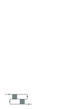
FIG. 1.: Diagrams contributing to the Green function for the chiral unitary class. The dark-shaded regions represent a diffuson-type ladder.

For the chiral orthogonal and symplectic classes, we can anticipate the $1/E$ term contribution. This is indeed the case and we can express the $1/E$ term contribution as Fig.2. We note that the singular contribution comes from the cooperon-type ladder and the diffusion ladder contribution is the nonsingular one. We obtain the Green function as

$$\Bigl{<}\mbox{tr}\,G^{(R)}(E)\Bigr{>} = -i\,\frac{\pi}{\Delta}\,\biggl{[}\,1+\frac{i\alpha}{2\pi E/\Delta}$$ (92)

$$+\frac{5}{16(\pi E/\Delta)^{2}}+\cdots\,\biggr{]}.$$

We confirm that the first three terms coincide again with the supersymmetric calculation.

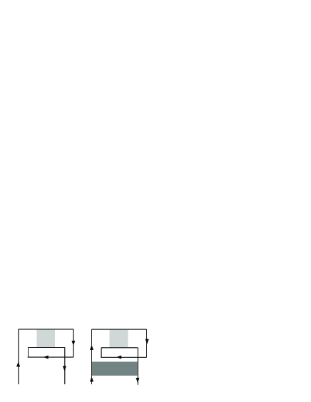
FIG. 2.: Diagrams contributing to the Green function for the chiral orthogonal and symplectic classes. The light-shaded regions represent a cooperon-type ladder.

B Two-point level-correlation function

The leading order contributions to the twp-point level-correlation function can be expressed with the same diagram as the traditional classes (two diffusons and two cooperons).[21] For the chiral unitary case, we take the diffuson-type diagram only. Calculating these diagrams, we can derive Eq.(69).

IV Conclusions

In this paper, we have formulated the impurity perturbative expansion for chiral symmetric disordered systems. For three chiral classes, we calculated the large-$E$ and small-$E$ behavior of the density of state and the large-$E$ behavior of the two-point level-correlation function. The deviations from the universal function are obtained in which we find the effects similar to the weak localization effects for the traditional classes. We calculate these deviations by considering the nonzero-$k$ modes explicitly. Alternatively, one can, in principle, integrate out the nonzero modes from the start and get the effective action for the zero mode. Then, working with this action should give the same results.

For the behavior at the large energy, we can interpret the results diagrammatically. We see that the diffuson and cooperon modes generate the nontrivial contribution to the level correlation functions. We have the diffuson and cooperon contributions in the advanced-advanced (retarded-retarded) channel in addition to the usual ones.

For the chiral unitary and orthogonal classes we get the small-$E$ behavior that could be interpreted as a weakening of the repulsion between a pair of levels with the energy $\pm E$. For the chiral symplectic case, however, we get a result with opposite tendency whose intuitive explanation remains an open problem. These results imply the divergence of the density of states at the band center for the chiral unitary and orthogonal classes and the vanishing for the chiral symplectic class in the thermodynamic limit. For the chiral unitary class, this divergence is observed by the renormalization group calculation.[13] The calculations for the other classes are future problems.

If once we derive the nonlinear sigma model and formulate the perturbation theory, it is easy to use this calculation to several applications such as the study of the wave function statistics and the renormalization group equations. These are currently under intensive study.

REFERENCES

- [1] M. R. Zirnbauer, J. Math. Phys. 37, 4986 (1996). The localization problem for all symmetric spaces was first considered in: S. Hikami, Prog. Theor. Phys. 64, 1466 (1980).
- [2] A. Altland and M. R. Zirnbauer, Phys. Rev. B 55, 1142 (1997).
- [3] A. Altland and B. D. Simons, Nucl. Phys. B 562, 445 (1999).
- [4] V. Kalmeyer and S.-C. Zhang, Phys. Rev. B 46, 9889 (1992); B. I. Halperin, P. A. Lee, and N. Read, Phys. Rev. B 47, 7312 (1993).
- [5] L. B. Ioffe and A. I. Larkin, Phys. Rev. B 39, 8988 (1989); N. Nagaosa and P. A. Lee, Phys. Rev. Lett. 64, 2450 (1990).
- [6] E. V. Shuryak and J. J. M. Verbaarschot, Nucl. Phys. A 560, 306 (1993).
- [7] K. Slevin and T. Nagao, Phys. Rev. Lett. 70, 635 (1993).
- [8] J. J. M. Verbaarschot and I. Zahed, Phys. Rev. Lett. 70, 3852 (1993).
- [9] M. Ando, A. Endo, S. Katsumoto, and Y. Iye, Physica B 284-288, 1900 (2000).
- [10] K. Takahashi and S. Iida, Nucl. Phys. B 573, 685 (2000); Nucl. Phys. A 670, 60 (2000).
- [11] K. Efetov, Adv. Phys. 32, 53 (1983); Supersymmetry in Disorder and Chaos (Cambridge Univ. Press, Cambridge, 1997).
- [12] A. V. Andreev, B. D. Simons, and N. Taniguchi, Nucl. Phys. B 432, 487 (1994).
- [13] R. Gade, Nucl. Phys. B 398, 499 (1993).
- [14] T. Guhr, T. Wilke, and H. A. Weidenmüller, Phys. Rev. Lett. 85, 2252 (2000).
- [15] D. Taras-Semchuk and K. B. Efetov, Phys. Rev. Lett. 85, 1060 (2000).
- [16] J. C. Osborn, D. Toublan, and J. J. M. Verbaarschot, Nucl. Phys. B 540, 317 (1999); P. H. Damgaard, J. C. Osborn, D. Toublan, and J. J. M. Verbaarschot, Nucl. Phys. B 547, 305 (1999); D. Toublan and J. J. M. Verbaarschot, Nucl. Phys. B 560, 259 (1999).
- [17] V. E. Kravtsov and A. D. Mirlin, Pis’ma Zh. Eksp. Teor. Fiz. 60, 645 (1994) [JETP Lett. 60, 656 (1994)].
- [18] Y. V. Fyodorov and A. D. Mirlin, Phys Rev. B 51, 13403 (1995).
- [19] J. Verbaarschot, Nucl. Phys. B 426, 559 (1994).
- [20] T. Nagao and P. J. Forrester, Nucl. Phys. B 435, 401 (1995).
- [21] B. L. Altshuler and B. I. Shklovskii, Zh. Eksp. Teor. Fiz. 91, 220 (1986) [Sov. Phys. JETP 64, 127 (1986)].