Lattice Resistance and Peierls Stress in Finite-size Atomistic Dislocation Simulations

Abstract

Atomistic computations of the Peierls stress in fcc metals are relatively scarce. By way of contrast, there are many more atomistic computations for bcc metals, as well as mixed discrete-continuum computations of the Peierls-Nabarro type for fcc metals. One of the reasons for this is the low Peierls stresses in fcc metals. Because atomistic computations of the Peierls stress take place in finite simulation cells, image forces caused by boundaries must either be relaxed or corrected for if system size independent results are to be obtained. One of the approaches that has been developed for treating such boundary forces is by computing them directly and subsequently subtracting their effects, as developed in Shenoy and Phillips [1]. That work was primarily analytic, and limited to screw dislocations and special symmetric geometries. We extend that work to edge and mixed dislocations, and to arbitrary two-dimensional geometries, through a numerical finite element computation. We also describe a method for estimating the boundary forces directly on the basis of atomistic calculations. We apply these methods to the numerical measurement of the Peierls stress and lattice resistance curves for a model aluminum (fcc) system using an embedded-atom potential [2].

1. Introduction

Dislocation simulations at the atomistic level are affected by boundary forces, except in very special cases. This is equally true whether the simulations are based on semi-empirical potentials or density functional theory. Two examples which serve to illustrate the potentially disastrous influence of such boundary forces are: (1) To estimate the Peierls stress for a given system, that is the applied stress needed to move a straight dislocation in an otherwise perfect crystal. (2) To simulate the bow-out of a pinned dislocation under an applied stress.

If one simulates a single dislocation in a finite cell, then the boundary conditions imposed on that cell will determine the nature of the resulting boundary forces. One common type of boundary condition for a single dislocation is to fix all atoms whose distance from the dislocation core exceeds some critical radius at their positions as given by the linear (anisotropic) elastic solution for the dislocation of interest. This assumes that the linear elastic solution is accurate at long distances, which is a good assumption in many cases for a straight undissociated dislocation at a fixed position. To determine the Peierls stress the dislocation must be moved, however. After the dislocation has moved, the locations of the atoms in the fixed region will not be consistent with the elastic field of the dislocation in its new position.

In such a simulation, the dislocation is moved in the cell by applying a slowly increasing external stress. This external applied shear stress is simulated by applying the appropriate strain increment to all of the atoms, and, upon relaxing the free region, the fixed positions of the atoms in the exterior ring impose the desired stress on the free region. The minimum applied stress necessary to jump the dislocation out of its initial Peierls well, the apparent Peierls stress, will be overestimated because not only must the applied stress overcome the intrinsic lattice resistance, but the force due to the boundary as well.

At least two methods have been used to obtain accurate estimates of the Peierls stress of an atomistic model in cases where the boundary forces are important. One method is to relax the boundary forces through flexible boundary conditions [3]. The method we use here, developed by Shenoy and Phillips [1], [referred to hereafter as (I)], is to determine the boundary force contribution and correct for it. While this method is less elegant than the flexible boundary condition approach, it does not require any changes to the simulations themselves. We believe that this will make it useful to researchers in many cases where either the importance of boundary forces have not yet been determined, where implementing the flexible boundary condition is not an efficient allocation of effort, or where a “rough and ready” approach is needed as a starting point.

The boundary force correction approach also has one valuable capability that flexible boundary conditions does not. If the boundary forces are fully relaxed, the dislocation will jump as soon as the Peierls stress is reached. This creates a limitation on the part of the lattice resistance curve that can be measured. Using fixed boundary conditions, although the lattice resistance will begin to decrease after the Peierls stress is reached, the boundary resistance is monotonically increasing. The dislocation will not jump until the total resistance begins to decrease. After subtracting the boundary force to obtain the lattice resistance, some portion of the lattice resistance curve beyond the area accessible to the flexible boundary condition approach is maintained. In fact, if the boundary forces are large enough, it is possible that the entire lattice resistance curve will become accessible. This is a useful, but imperfect benefit, because the small cell required to view the entire lattice resistance curve is likely to also be small enough to introduce distortions, even after correction of the boundary forces. In the work reported here, only for the smallest cells is any data obtained for the lattice resistance curve in the areas that would otherwise be inaccessible.

A third possiblity which has been used for measuring the static Peierls stress of fcc dislocations is fully periodic boundary conditions [4]. Since fully periodic boundary conditions are inconsistent with the existence of a net Burgers vector in the simulation cell, a dislocation dipole or quadrupole must be used [5]. As discussed in ref. [5] a disadvantage in this case are the interactions between the dislocations and with their images. In measuring the Peierls stress based on the motion of a dislocation in response to an applied stress, the dislocations of opposite Burgers vector making up the dipole or quadrupole will experience equal and opposite Peach-Kohler forces, and their relative positions will change. While the long range nature of the forces between the dipoles and images will complicate any correction for the forces between the dislocations, these could be computed in linear elasticity based on the measured locations of the dislocations or partials. For a simulation cell of the same size, the forces between the dislocations (including the periodic images) will be stronger than the boundary forces in our configuration. This increases the possibility of distortion of the dislocation core. In the case of an fcc dislocation split into Shockley partials, there will be a force compressing or expanding the partials which will be much stronger than in the configuration used here. The extent to which the resulting simulation size dependence of the partial separation will make the Peierls stress size dependent is unclear.

A fourth possible approach to measuring the Peierls stress would be to use periodic boundary conditions in the glide direction as well as the line direction, but with walls of fixed (or partially fixed) atoms on each side in the third direction. We are aware of dynamic studies of dislocation motion in such configurations [6, 7, 8, 9], but not of any measurements of the static Peierls stress. Such a configuration can contain a single dislocation, avoiding some of the hazards of the previous approach. Compared to our approach, in such a configuration the forces generated by the fixed boundaries will have no net component in the glide direction. As in the case of fully periodic boundary conditions, for a simulation cell of similar size, the forces between the periodic images of the dislocation will be stronger than the boundary forces in our configuration, but again the net force on the dislocation should be zero. The possibilities of core distortion are again significant, however, and similar to the case of full periodic boundary conditions.

In (I) the boundary forces are computed analytically for a screw dislocation, and it is shown that this boundary force correction allows for computation of a size-independent Peierls stress and for the simulation of bow-out. The analytical solution presented is limited to the screw dislocation, and is also limited to a circular geometry for the case of isotropic elastic moduli. For anisotropic elastic moduli it is limited to an elliptical geometry. We have extended the computation of the boundary forces using the approach developed in (I) in such a way that it can be used for both dislocations of other characters and to other geometries. In fact, we introduce two numerical schemes which allow for the determination of the boundary force correction. One method is based upon linear elasticity and is implemented numerically using the finite-element method, and it provides a more general numerical implementation of the ideas presented in (I). The other method is a measurement of the energy associated with the boundary-force directly on the basis of an atomistic description of the total energy.

We apply our methods to measurements of the lattice resistance curves and Peierls stresses for dislocations in aluminum, using the Ercolessi and Adams glue potential [2]. The estimates of the lowest order term in the boundary-force from the finite element method elasticity computations and from atomistics are in good agreement. The computed boundary-force predictions allow estimates of the Peierls stress that show much less size dependence than computations done without such corrections. This makes it possible for us to measure, with reasonable accuracy, the Peierls stress for the easy-glide edge dislocation in this model system, which is roughly $6\!\times\!10^{-5}\mu$. In the absence of boundary corrections, this value is overestimated by a factor varying between four and two. (The degree to which this stress is overestimated depends on the size of the simulation cell, and is off by a factor of four for a cell with a diameter of $100$ Å, and by a factor of two even for a cell with a diameter of $180$ Å.) The magnitude of the corrections vary with the dislocation character. For the screw dislocation, where the Peierls stress is roughly $5\!\times\!10^{-4}\mu$, the overestimate caused by ignoring boundary force corrections is significantly smaller than for the edge dislocation.

2. The boundary force on a dislocation.

In order to correct for boundary force effects we must understand them in quantitative terms and be able to compute them accurately. Fortunately, for the case of an isotropic screw dislocation in a cylindrical body, a closed form analytic result is available from an image method [(I)]. Consider a screw dislocation displaced a distance $d$ from the center of a cylindrical region of radius $R$ as depicted in figure 1. We suppose that the boundary conditions imposed at the surface are fixed displacements, corresponding to the isotropic linear elastic solution for the dislocation located at the center. We wish to obtain the excess energy of the system with the dislocation located at $P$, where it is displaced by $d$, compared to the system with the dislocation at the center, $O$. To effect the calculation of this excess energy, we assume the material can be characterized using isotropic linear elasticity.

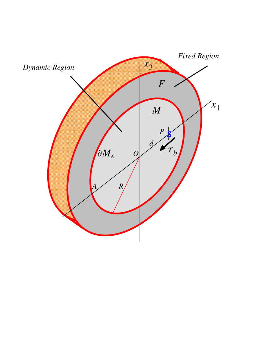
Figure 1: Cell geometry illustrating both the free and fixed regions (taken from Ref. [1]).

In figure 2 we illustrate the image solution. By adding a screw dislocation at a point Q, with the same Burgers vector, it is possible to create an infinite medium problem where the displacements at the edge of the circle caused by the dislocations at P and at Q satisfy the relevant boundary conditions which are the displacements for a single dislocation at position $O$.

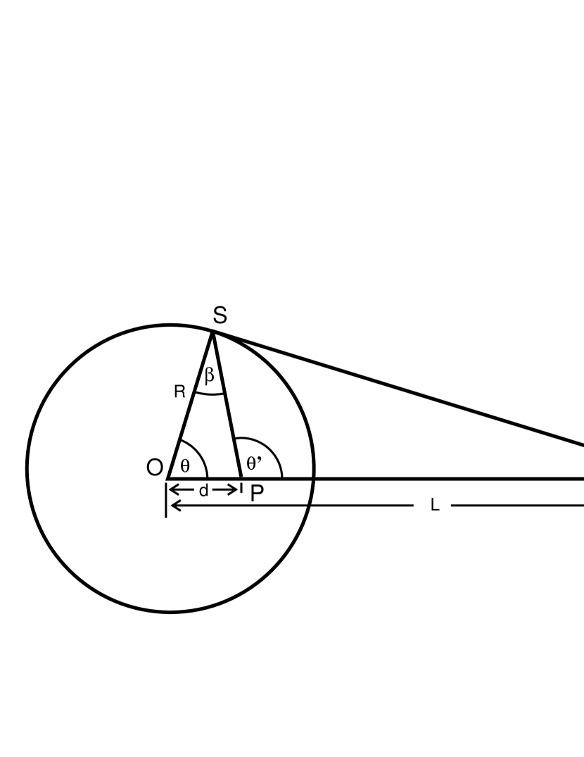
Figure 2: Image solution

Consider a particular point on the circle, given by an angle $\theta$. Let ${\theta^{\prime}}$ be the angle at $P$, and $\phi$ the angle at $Q$. For the isotropic screw dislocation the displacements are entirely in the $x_{2}$ direction, which is parallel to the dislocation line itself, and perpendicular to the plane of the paper in figure 2. For the simple case of a screw dislocation, the fixed displacement at point S due to a dislocation at the origin is $-b\theta/2\pi$ [10], and we note that these are the displacements that serve as our boundary condition. The displacement caused by a dislocation at $P$ is $-b{\theta^{\prime}}/2\pi$. Taking the surface at which the displacement jump occurs for the dislocation at $Q$ to its right along the positive $x_{1}$ axis, the displacement it causes is $b\phi/2\pi$. From a physical perspective, we now require that the superposition of the fields due to the dislocations at $P$ and $Q$ result in a displacement field that is entirely equivalent to that due to the single dislocation at $O$. From a mathematical perspective, this statement is

$${\theta^{\prime}}-\phi =\theta,$$ (1)

$$\phi ={\theta^{\prime}}-\theta.$$ (2)

This determines the point $Q$ and the distance $L$, which at this stage depend on $\theta$. Notice that there are further geometric constraints such as

$$\beta={\theta^{\prime}}-\theta=\phi.$$ (3)

The triangles $OQS$ and $OSP$ are therefore similar, and we have

$$\frac{L}{R} =\frac{R}{d}$$ (4)

$$L =\frac{R^{2}}{d}.$$ (5)

Since $L$ is independent of $\theta$, the boundary condition is satisfied at all points on the circle. Because the dislocation at $P$ feels no force from its own elastic strain field, the total configurational force on it is the force caused by the dislocation at $Q$, and is equal to [10]

$$F_{\mbox{\scriptsize b}}/l =-\frac{\mu b^{2}}{2\pi}\frac{1}{L-d}$$ (6)

$$=-\frac{\mu b^{2}}{2\pi}\left(\frac{d}{R^{2}-d^{2}}\right).$$ (7)

We note that the image dislocation is at the same location, but opposite in sign, to the image dislocation relevant to the same cylindrical geometry, but with free-surface boundary conditions [10].

This force profile can be used in turn to characterize the energetics of the system as a result of the frozen boundaries. Indeed, integration over this force-displacement relation yields the extra elastic energy generated by displacing the dislocation a distance $d$ from the center of the cylinder as

$$E/l=-\frac{\mu b^{2}}{4\pi}\ln\left(1-\frac{d^{2}}{R^{2}}\right).$$ (8)

On the other hand, for dislocations other than the screw dislocation considered above or for anisotropic elasticity, we do not expect such a simple, closed-form solution. Noting, however, that for this particular solution the energy depends only on $d/R$, not on $d$ and $R$ separately, and has a convergent power series expansion in the relevant range, $-1<d/R<1$, in our subsequent developments we have been emboldened to fit our numerical results to a power series in $d/R$.

For our model aluminum system, the screw dislocation splits (approximately) into Shockley partials. While we cannot use the image solution to handle the edge portions of the partials, it can be used to compute the boundary force for the non-physical case of pure screw partials, each with Burgers vector equal to $b/2$. This is discussed in Appendix A. (In general all of the treatment of the affects of partial splitting have been placed in Appendix A, in hopes of making the story in the main text more focused.)

The use of equation (7) to determining the lattice resistance curve was developed in (I). There it was assumed that total configurational force on the displaced dislocation has three contributions, the Peach-Kohler force corresponding to the applied shear stress, which is independent of $d$; the boundary force, which in linear elasticity (for a perfect dislocation) depends only on $d/R$; and the lattice resistance, which is assumed to depend periodically on $d$, and to be independent of $R$. As discussed in Appendix A, the splitting of the dislocations into Shockley partials allows the boundary force to depend on both $d/R$, and $s/R$, where $s$ is half the distance between the partials. As in (I) we assume that the partial separation is fixed during the course of the dislocation’s journey across the Peierls energy landscape.

For a configuration of the system where the dislocation is at static equilibrium, we then have

$$F_{\mbox{\scriptsize app}}+F_{\mbox{\scriptsize b}}(d)+F_{\mbox{\scriptsize L}}(d)=0,\hskip 30.00005pt$$ (9)

The applied force is given by the Peach-Kohler formula. If, for a given applied force, we can measure the displacement $d$ of the dislocation from the center of the cell, and if we can compute the boundary force, then subtracting the boundary force we obtain the value of the lattice resistance, $F_{\mbox{\scriptsize L}}(d)$. (Our measurement of the position of the dislocation is discussed below.) By varying the applied stress we obtain the curve $F_{\mbox{\scriptsize L}}(d)$, which allows us to determine not only the Peierls stress, but to map out the Peierls force landscape as well.

An alternative way to view $F_{\mbox{\scriptsize b}}(d)$ is to say that the elastic stress to be used in the Peach-Kohler formula is the applied stress less the amount of stress relieved through the movement of the dislocation [11, 3]. Using this approach Simmons et al. [11] were able to obtain the correct scaling for the leading term in $F_{\mbox{\scriptsize b}}(d)$, that is $\mu bd/R^{2}$, and a reasonable estimate of its numeric coefficient (which did not vary with dislocation character).

Before embarking on a precise numerical assessment of our results, we first need to consider the validity of the assumptions leading to equation (9). As the dislocation is displaced with respect to the periodic lattice, the core configuration will change. Because the configurational forces generated by the applied stress and the boundary conditions are both long-range elastic effects, we expect the assumption that they are unaffected by this periodic change in the core structure to be negligible for $d\ll R$. It is possible that the core configuration will be affected by the boundary forces, however, and that this will cause some distortion of the lattice resistance force as the dislocation moves. As discussed in (I) this is certainly possible for the partial separation distance, since the boundary forces on the two partials will tend to have a net constrictive element. Clearly equation (9) is an assumption we need to validate for our system.

As described above, our results will provide the curve $F_{\mbox{\scriptsize L}}(d)$. By assumption this will depend periodically on $d$ and be independent of $R$. By testing these predictions in our results, we will find that the underlying assumptions are appropriate for all of our dislocations except the edge, and are reasonable for the edge dislocation, except for our smallest cell.

3. Computation of Boundary Force Correction Coefficients

3.1. Setup

As in (I) we consider the problem of modeling a straight dislocation in a finite cylindrical cell. The geometry, shown in figure 1, has $x_{2}$ as the line direction of the dislocation, and the $x_{1}$–$x_{2}$ plane as the slip plane. In the simulation there is a dynamic region of radius R, and a fixed region outside R, with periodic boundary conditions in the $x_{2}$ direction. A dislocation is introduced at $O$, the center of the cell, using the continuum anisotropic linear elastic solution for either a single dislocation or for two Shockley partials. This initial configuration is relaxed using energy minimization, by allowing the atoms in the free region to move. The atoms in the fixed region remain at the locations corresponding to the elasticity solution. This relaxed dislocation at the center of the cell serves as a reference configuration.

The objective of our analysis is to examine the response of a dislocation to an applied stress, while correcting for the contaminating influence of boundaries. We model the application of a homogeneous shear stress by moving the atoms according to the homogeneous strain which produces the desired stress under linear elasticity. Keeping the atoms in the fixed region at these strained positions, the atoms in the dynamic region are relaxed. The dislocation now moves to a new position $P$ which (locally) minimizes its energy. We assume that the structure of the dislocation core does not change, and we therefore treat the distance $d=\overline{OP}$ as the sole configurational parameter.

Consider, then, the energy per unit length, $E(d)$, of the dislocation as a function of its distance $d$ from the center of the cylindrical cell. As in (I) we assume that this configurational energy consists of four parts

$$E(d)=E_{\mbox{\scriptsize ref}}-db\tau_{\mbox{\scriptsize app}}+E_{\mbox{\scriptsize L}}(d)+E_{\mbox{\scriptsize b}}(d),$$ (10)

where $E_{\mbox{\scriptsize ref}}$ is a constant representing the energy of the reference configuration when the dislocation is at the origin; $\tau_{\mbox{\scriptsize app}}$ is the resolved shear stress; $E_{\mbox{\scriptsize L}}$ is the Peierls energy, assumed to be periodic in $d$; and $E_{\mbox{\scriptsize b}}$ is the energy associated with the boundary force. The first three terms appear in the energy of a dislocation in an infinite medium, while $E_{\mbox{\scriptsize b}}$ is the result of the mismatch between the imposed displacement boundary conditions and the strain field the dislocation would generate at its position $d$ in an infinite medium. And, as in (I), we define

$$\Delta E=E_{\mbox{\scriptsize b}}(d)-E_{\mbox{\scriptsize b}}(0).$$ (11)

Motivated by the analytic structure of the image solution discussed above, we will couch our estimates for the energy caused by the finite boundaries (for small $d/R$) in the form

$$\Delta E=\frac{\mu b^{2}}{8\pi^{2}}\left[A\left(\frac{d}{R}\right)^{2}+C\left(\frac{d}{R}\right)^{3}+B\left(\frac{d}{R}\right)^{4}+O((d/R)^{5})\right].$$ (12)

Here $\mu$ is taken as $\{C_{44}^{2}+[(C_{11}-C_{12})/2]^{2}\}^{1/2}$, the value of $\mu$ which gives the correct logarithmic prefactor for the line energy of the (anisotropic) screw dislocation. By symmetry, odd powers can only occur for the case in which a mixed-character dislocation is treated as split into Shockley partials (as the partials then have different characters). For the isotropic screw dislocation, the image solution then gives $A=2\pi;B=\pi$.

In the application of this expansion in powers of $d/R$ to the simulations there is some ambiguity in the measurement of both $d$ and $R$. The measurement of $d$ is discussed below. In the analytic elasticity solution using the image solution, the fixed displacement boundary conditions are specified at all points on the circle of radius $R$. In the simulations, the fixed atoms are necessarily discrete. The specification of fixed displacement boundary conditions at all the atomic positions which lie outside a circle of radius $R$ provides a ‘softer’ boundary condition than if all points on the circle of radius $R$ had specified displacements, making the effective $R$ that best fits the expansion slightly greater than the $R$ used to specify the fixed region. Except as otherwise stated, in this work we have used the nominal $R$ for the simulations. (It is also the case that the nominal $R$ is ambiguous in that it could equally well be any value between the value of $r$ for the outermost free atom and the value of $r$ for the innermost fixed atom. This difference is very small, and is small compared to the difference between the ‘nominal’ and the ‘effective’ $R$.

3.2. Computing Coefficients in Linear Elasticity

In order to correct for the finite system size by using the force balance equation, equation (9), we need to evaluate the boundary force, which we derive from the configurational energy $\Delta E$. We estimate $\Delta E$ in this section in linear elasticity, using a finite element method numerical solution. In the following section we discuss a second approximate scheme for the determination of $\Delta E$ using atomistic simulations.

The evaluation of $\Delta E$ in linear elasticity follows (I) exactly, except for the method of computation. The energy difference $\Delta E$ is the excess of the elastic energy $E_{2}$ of the system with the dislocation at $P$, over its energy $E_{1}$ with the dislocation at $O$. The boundary conditions at the edge of the finite cylinder are fixed displacements, given by the linear elastic (Volterra) solution for the dislocation at $O$. This element of the boundary conditions is the same whether the dislocation is at $O$ or at $P$. The boundary conditions on the slip surface are given by $[[{{\bf u}}]]={{\bf b}}$, but the slip surface is extended from $O$ to $P$ when the dislocation moves to $P$. (Or retracted from $O$ to $P$ if $d<0$.) This element of the boundary conditions, therefore, differs by a displacement jump between the two configurations. We know the stress, strain and displacement fields when the dislocation is at $O$ analytically, from the sextic formulation of Eshelby et al. [12, 13, 14, 15]. The energy for the system at $O$ is then simply

$$E_{1}={\frac{1}{2}}\int_{M}{\boldsymbol{\sigma}}_{O}\cdot{\boldsymbol{\epsilon}}_{O}{\,\mbox{d}}V,$$ (13)

where elastic variables with a subscript $O$ refer to the elastic fields of a dislocation at $O$ in an infinite medium. As written, $E_{1}$ has the normal logarithmic divergence at $O$. We handle this in the customary way, excluding a cylinder of radius $r_{c}$ at $O$, and introducing a dependence of $E_{1}$ on $r_{c}$ [10]. As in (I), we assume the same value of $r_{c}$ in evaluating $E_{1}$ and $E_{2}$, in which case the dependence on $r_{c}$ cancels in taking the difference $E_{2}-E_{1}$, which is independent of $r_{0}$, as will be seen below.

When the dislocation is at $P$ we do not have analytic solutions for the displacement, stress and strain fields available. We wish to apply the finite element method to numerically solve the elasticity problem posed by the difference between the two configurations with the dislocation at $O$ and $P$. However, rather than attempt to handle the displacement jump boundary condition in the finite element method, it is convenient to separate the problem into two problems, one of which has only (continuous) fixed displacement boundary conditions, and one of which has analytic solutions for the fields available. We therefore also consider a third set of elastic fields, those for a dislocation at $P$ in an infinite medium. (They will be denoted with a subscript $P$, while the equilibrium fields for the configuration with the dislocation at $P$ subject to our actual boundary conditions will have no subscript.) We therefore define

$${{\bf u}}_{\Delta}={{\bf u}}-{{\bf u}}_{P}.$$ (14)

The interpretation of this is that the displacement field due to the dislocation when it is at $P$ is that of a dislocation situated at $P$ in an infinite body, plus a correction field ${{{\bf u}}_{\Delta}}$ which adjusts ${{\bf u}}_{P}$ so as to be consonant with the boundary conditions. The boundary conditions on ${{\bf u}}$ are

$${{\bf u}}= {{\bf u}}_{O}\hskip 30.00005pt\mbox{ on }{\partial M_{e}}$$

$$[[{{\bf u}}]]= {{\bf b}}\hskip 30.00005pt\mbox{ on }{\partial M_{s^{\prime}}}.$$ (15)

Since ${{\bf u}}_{P}$ also has $[[{{\bf u}}_{P}]]={{\bf b}}$ on ${\partial M_{s^{\prime}}}$, the boundary conditions for ${{{\bf u}}_{\Delta}}$ are

$${{{\bf u}}_{\Delta}}= {{\bf u}}_{O}-{{\bf u}}_{P}\hskip 30.00005pt\mbox{ on }{\partial M_{e}}$$

$$[[{{{\bf u}}_{\Delta}}]]= {\bf 0}\hskip 30.00005pt\mbox{ on }{\partial M_{s^{\prime}}}.$$ (16)

Thus ${{{\bf u}}_{\Delta}}$ is the solution to an elasticity boundary value problem without singularities, and can be solved by the finite element method. The fields ${{\bf u}}_{P}$, and the related stress and strain fields are essentially the same as the fields ${{\bf u}}_{0}$ save that they have been translated.

We now have

$$E_{2}={\frac{1}{2}}\int_{M}({\boldsymbol{\sigma}}_{P}+{\boldsymbol{\sigma}}_{\Delta})\cdot({\boldsymbol{\epsilon}}_{P}+{\boldsymbol{\epsilon}}_{\Delta}){\,\mbox{d}}V,$$ (17)

where

$${\boldsymbol{\epsilon}}_{\Delta}= \nabla{{\bf u}}_{\Delta}$$

$${\boldsymbol{\sigma}}_{\Delta}= {\bf C}:{\boldsymbol{\epsilon}}_{\Delta},$$ (18)

where C is the elastic stiffness tensor.

In principle, these are satisfactory forms in which to compute the energy difference. However, for purposes of numerical computation it is preferable to manipulate $E_{1}-E_{2}$ into a form where the portions not involving ${{{\bf u}}_{\Delta}}$ are reduced from volume (effectively surface) integrals to an analytic piece plus a line integral. Among other advantages, this eliminates the logarithmic divergences at $O$ and $P$, as the cancellation is handled in the analytic piece. The rest of this section, which follows (I), develops this form of $E_{1}-E_{2}$.

The energy of the dislocation in the finite cylinder can be computed as the work done by applying tractions on all relevant surfaces to obtain the final displacements, where these surfaces must include not only the exterior surface of the cylinder, but also a slip surface where the displacement discontinuity of the dislocation is introduced. We choose the plane $\overline{AP}$, denoted ${\partial M_{s^{\prime}}}$ ($\overline{AO}$, denoted ${\partial M_{s}}$) for the slip surface when the dislocation is at $P$ ($O$, respectively). We denote the exterior of the cylinder as ${\partial M_{e}}$. Notice that, except for the case of a screw dislocation, the surface of the cylinder will have a step at $A$ either before or after the dislocation is inserted. This step is the same in both configurations, however, and it will not contribute to $\Delta E$. For convenience in numerical computation, we assume that the cylinder started with a step at $A$, which is eliminated by the insertion of the dislocation. The elastic energy of the system with the dislocation at $O$ is given by [(I)],

$$E_{1}={\frac{1}{2}}{\int_{\partial M_{s}}}{{\bf t}}_{O}\cdot{[[{{\bf u}}_{O}]]}{\,\mbox{d}}S+{\frac{1}{2}}{\int_{\partial M_{e}}}{{\bf t}}_{O}\cdot{{\bf u}}_{O}{\,\mbox{d}}S,$$ (19)

where ${{\bf t}}_{O}$ is the traction at the surface caused by the presence of the dislocation at $O$ in an infinite medium, ${{\bf u}}_{O}$ is the displacement at the exterior surface, and ${[[{{\bf u}}_{O}]]}$ is the displacement jump at the slip plane. (We have ${{\bf t}}_{O}=\boldsymbol{\sigma}_{O}\cdot{\bf n}$, where $\boldsymbol{\sigma}_{O}$ is the stress tensor, and ${\bf n}$ the outward normal for the exterior surface and is in the positive $x_{3}$ direction at the slip plane.) ${[[{{\bf u}}_{O}]]}$ is the jump in displacement experienced on crossing the slip plane in the opposite direction to ${\bf n}$, and is equal to ${{\bf b}}$, the Burgers vector. The line direction here is in the positive $x_{2}$ direction, and our choice of directions is that of (I).

Letting ${{\bf t}}$ be the traction associated with ${{\bf u}}$ and ${{{\bf t}}_{\Delta}}$ be the traction associated with ${{{\bf u}}_{\Delta}}$, we have by linearity that

$${{{\bf t}}_{\Delta}}={{\bf t}}-{{\bf t}}_{P}.$$ (20)

The energy of the configuration with the dislocation at $P$ is now

$$E_{2}= {\frac{1}{2}}{\int_{\partial M_{s^{\prime}}}}{{\bf t}}\cdot{[[{{\bf u}}_{P}]]}{\,\mbox{d}}S+{\frac{1}{2}}{\int_{\partial M_{e}}}{{\bf t}}\cdot{{\bf u}}_{O}{\,\mbox{d}}S$$ (21)

$$= {\frac{1}{2}}{\int_{\partial M_{s^{\prime}}}}({{\bf t}}_{P}+{{{\bf t}}_{\Delta}})\cdot{[[{{\bf u}}_{P}]]}{\,\mbox{d}}S+{\frac{1}{2}}{\int_{\partial M_{e}}}({{\bf t}}_{P}+{{{\bf t}}_{\Delta}})\cdot({{\bf u}}_{P}+{{{\bf u}}_{\Delta}}){\,\mbox{d}}S.$$ (22)

By the reciprocal theorem

$${\frac{1}{2}}{\int_{\partial M_{s^{\prime}}}}{{{\bf t}}_{\Delta}}\cdot{[[{{\bf u}}_{P}]]}{\,\mbox{d}}S+{\frac{1}{2}}{\int_{\partial M_{e}}}{{{\bf t}}_{\Delta}}\cdot{{\bf u}}_{P}{\,\mbox{d}}S$$ (23)

$$= {\frac{1}{2}}{\int_{\partial M_{s^{\prime}}}}{{\bf t}}_{P}\cdot[[{{{\bf u}}_{\Delta}}]]{\,\mbox{d}}S+{\frac{1}{2}}{\int_{\partial M_{e}}}{{\bf t}}_{P}\cdot{{{\bf u}}_{\Delta}}{\,\mbox{d}}S$$

$$= {\frac{1}{2}}{\int_{\partial M_{e}}}{{\bf t}}_{P}\cdot{{{\bf u}}_{\Delta}}{\,\mbox{d}}S.$$

Hence, following (I) we have,

$$E_{2}= {\frac{1}{2}}{\int_{\partial M_{s^{\prime}}}}{{\bf t}}_{P}\cdot{[[{{\bf u}}_{P}]]}{\,\mbox{d}}S+{\frac{1}{2}}{\int_{\partial M_{e}}}{{\bf t}}_{P}\cdot{{\bf u}}_{P}{\,\mbox{d}}S$$

$$\mbox{}+{\int_{\partial M_{e}}}{{\bf t}}_{P}\cdot{{{\bf u}}_{\Delta}}{\,\mbox{d}}S+{\frac{1}{2}}{\int_{\partial M_{e}}}{{{\bf t}}_{\Delta}}\cdot{{{\bf u}}_{\Delta}}{\,\mbox{d}}S.$$ (24)

For computational purposes, we split $\Delta E=E_{2}-E_{1}$ into three parts.

$$\Delta E={\Delta E^{a}}+{\Delta E^{b}}+{\Delta E^{c}},$$ (25)

where

$${\Delta E^{a}}= {\frac{1}{2}}{\int_{\partial M_{s^{\prime}}}}{{\bf t}}_{P}\cdot{[[{{\bf u}}_{P}]]}{\,\mbox{d}}S-{\frac{1}{2}}{\int_{\partial M_{s}}}{{\bf t}}_{O}\cdot{[[{{\bf u}}_{O}]]}{\,\mbox{d}}S,$$ (26)

$${\Delta E^{b}}= {\int_{\partial M_{e}}}{{\bf t}}_{P}\cdot({{\bf u}}_{O}-{\frac{1}{2}}{{\bf u}}_{P}){\,\mbox{d}}S-{\frac{1}{2}}{\int_{\partial M_{e}}}{{\bf t}}_{O}\cdot{{\bf u}}_{O}{\,\mbox{d}}S,$$ (27)

$${\Delta E^{c}}= {\frac{1}{2}}{\int_{\partial M_{e}}}{{{\bf t}}_{\Delta}}\cdot{{{\bf u}}_{\Delta}}{\,\mbox{d}}S.$$ (28)

Of the three parts of this energy change, ${\Delta E^{a}}$ involves only the same terms used to compute the energy of a dislocation in an infinite medium. We take $r_{c}$ as a core cutoff radius, and K as the factor defined by Hirth & Lothe [10] eq. (13-83) for anisotropic elasticity. In isotropic elasticity

$$K=\mu\cos^{2}(\theta)+\frac{\mu}{1-\nu}\sin^{2}(\theta),$$ (29)

where $\theta$ is the angle the Burgers vector makes with the line direction. We then have, again following (I),

$$\frac{1}{l}{\frac{1}{2}}{\int_{\partial M_{s}}}{{\bf t}}_{O}\cdot{[[{{\bf u}}_{O}]]}{\,\mbox{d}}S= \frac{Kb^{2}}{4\pi}\int_{-R}^{-r_{c}}\frac{1}{-x_{1}}dx_{1}$$

$$= \frac{Kb^{2}}{4\pi}\ln\left(\frac{R}{r_{c}}\right),$$ (30)

$$\frac{1}{l}{\frac{1}{2}}{\int_{\partial M_{s^{\prime}}}}{{\bf t}}_{P}\cdot{[[{{\bf u}}_{P}]]}{\,\mbox{d}}S= \frac{Kb^{2}}{4\pi}\int_{-R}^{d-r_{c}}\frac{1}{d-x_{1}}dx_{1}$$

$$= \frac{Kb^{2}}{4\pi}\ln\left(\frac{R+d}{r_{c}}\right),$$ (31)

$${\Delta E^{a}}/l= \frac{Kb^{2}}{4\pi}\ln\left(\frac{R+d}{R}\right).$$ (32)

The reader is encouraged to examine appendix A for the more complex case of a dislocation split into partials.

The second piece of $\Delta E$,

$${\Delta E^{b}}={\int_{\partial M_{e}}}{{\bf t}}_{P}\cdot({{\bf u}}_{O}-{\frac{1}{2}}{{\bf u}}_{P}){\,\mbox{d}}S-{\frac{1}{2}}{\int_{\partial M_{e}}}{{\bf t}}_{O}\cdot{{\bf u}}_{O}{\,\mbox{d}}S,$$ (33)

involves only the known elastic fields for anisotropic dislocations in infinite media, evaluated on the boundary surface. We therefore evaluate ${\Delta E^{b}}/l$ directly as a numeric line integral around the circle.

The third piece of $\Delta E$ can be converted to a (effectively two-dimensional) volume integral

$${\Delta E^{c}}= {\frac{1}{2}}{\int_{\partial M_{e}}}{{{\bf t}}_{\Delta}}\cdot{{{\bf u}}_{\Delta}}{\,\mbox{d}}S$$ (34)

$$= {\frac{1}{2}}\int_{M}\boldsymbol{\sigma}_{\Delta}:\nabla{{{\bf u}}_{\Delta}}dV$$ (35)

$$= {\frac{1}{2}}\int_{M}\nabla{{{\bf u}}_{\Delta}}:{\bf C}:\nabla{{{\bf u}}_{\Delta}}dV,$$ (36)

where C is the elastic stiffness tensor. We compute ${{{\bf u}}_{\Delta}}$ as the solution to the relevant boundary value problem described above, using the finite element method, and so obtain ${\Delta E^{c}}/l$.

This treatment extends the implementation of the approach developed in (I) for the computation of the boundary force to edge and mixed dislocations, and will handle arbitrary two-dimensional geometries. The applications reported here are all for circular geometries, though we have also applied the method to rectangular geometries.

3.3. Computing the Quadratic Coefficient from Atomistics

The discussion given thus far has emphasized the use of the linear theory of elasticity to evaluate the force on a dislocation as a result of the boundary conditions to which the system has been subjected. However, as noted in the opening discussion of this paper, it is also possible to evaluate these boundary condition induced forces directly on the basis of atomistic calculations, and that is the charter of the present discussion. As in the elasticity computation, an energy approach to computing the configurational force is adopted. A dislocation is introduced into the simulation cell using the (anisotropic) linear elastic solution. The atoms in the exterior region are fixed at this solution, and the dislocation is relaxed. The potential energy function is then interrogated as to the total energy of the system, including that of the fixed atoms. This will be referred to as the energy of the reference configuration. This energy includes a large surface energy contribution, but it is a fixed value and will drop out of the differences in energy computed as the dislocation is moved.

The dislocation is then moved by a lattice vector, so that, if the lattice were infinite, the new configuration would have identical energy. To measure the boundary-condition contribution to the energy, we need to relax the free region of the simulation cell, subject to the condition that the dislocation stay at its new location. For mobile dislocations, if we relax all of the free atoms, the dislocation will move back to the center of the cell. We therefore freeze a small cylindrical region about the new location of the dislocation. Because the relaxed dislocation cores are extended in the slip plane, this frozen-core is chosen large enough to include the apparent centers of both partials. For all the simulations used to compute the boundary-force coefficient $A$ that was introduced in equation (12), the free region had a radius of 127 Å, and the fixed solution for the exterior region was the (anisotropic) linear elastic solution for a perfect dislocation. For a single value of the frozen-core radius the dislocation was moved in the slip direction by at least five different distances $d$ (in each direction) and the remaining free region relaxed. The excess of the energy over the reference configuration was then fit as a polynomial in $d/R$ giving an estimate of $A$. This estimate now depends on the frozen-core radius, $r_{\mbox{\scriptsize fc}}$. We therefore repeated this process for at least three values of $r_{\mbox{\scriptsize fc}}$ for each dislocation character, and extrapolated to $r_{\mbox{\scriptsize fc}}=0$ as an estimate of $A$ for the dislocation without a frozen-core. In performing this extrapolation we first considered fitting to $r_{\mbox{\scriptsize fc}}^{2}$ since the volume of the frozen-core scales with this parameter. The validity of this extrapolation scheme can be tested in turn by appealing to the case of the Lomer dislocation which is sessile and thus does not require the use of such a frozen-core region. (The Lomer dislocation is a dislocation with a Burgers vector of $a_{0}/2$ [1 -1 0] and a line direction of [1 1 0].) Indeed, the Lomer case supports the hypothesized $r_{\mbox{\scriptsize fc}}^{2}$ scaling and hence that has been used in the case of the glissile dislocations. figure 3 shows the quadratic fits to $r_{\mbox{\scriptsize fc}}^{2}$ used to develop the atomistic estimates of A. A similar attempt to measure B by extrapolation from frozen-core simulations did not produce useful estimates of B.

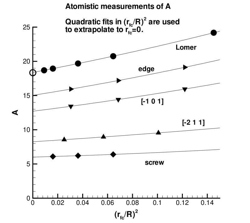
Figure 3: Extrapolation of the quadratic energy coefficient A as measured in frozen-core simulations to $r_{\mbox{\scriptsize fc}}=0$. The extrapolations are quadratic in $r_{\mbox{\scriptsize fc}}/R$. For the Lomer dislocation the open circle is from the simulations without any frozen-core.

figure 4 shows the values of the coefficient $A$ of the quadratic term in the boundary-force energy for various dislocations as obtained using finite element computations, showing the difference between isotropic and anisotropic elasticity, and from the atomistic measurement. There is a significant difference in the boundary force coefficient between the (glissile) edge dislocation and the Lomer dislocation, with A differing by 20% when anisotropic linear elasticity is used. Given the close approximation of aluminum to isotropic elastic constants this is rather large. By comparison, the long-range portion of the dislocation line energy differs by only 2.5 % between the Lomer dislocation and the glissile edge dislocation. We also note that the atomistic values for ‘A’ are slightly less than the values from anisotropic elasticity. One cause for this discrepancy is the ‘softer’ boundary condition of the atomistic simulations. On the other hand, given the severe differences in the calculational philosophy behind our two schemes [i.e. i) elasticity using finite elements and ii) direct atomistic evaluation of the boundary force] the level of agreement between the two schemes is remarkable.

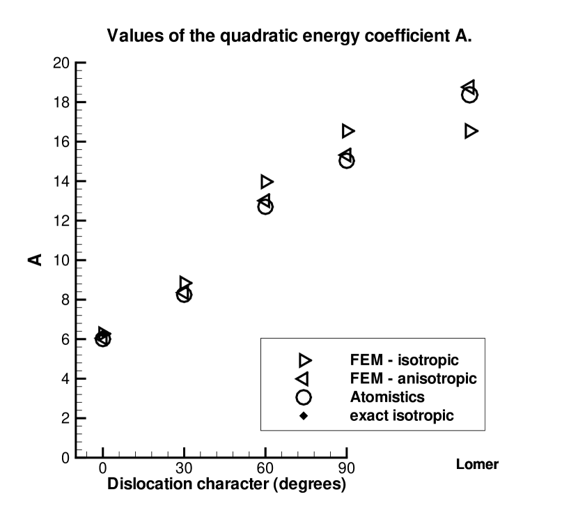
Figure 4: Quadratic coefficient in the boundary-force energy. This figure shows the different approximations to the quadratic boundary force coefficient including isotropic elasticity, anisotropic elasticity, and direct atomistic calculation. The results are shown for five $a_{0}/2[1\bar{1}0]$ dislocations; four are in the $(111)$ slip plane, labeled by the angle between the line direction and the Burgers vector, with the screw dislocation labeled 0 and the edge dislocation labeled 90. A sessile edge dislocation, the Lomer dislocation, is also shown.

4. Application of Boundary Force Correction

The usefulness of the boundary force corrections proposed in (I) depends on an accurate computation of the boundary force acting on a dislocation. To compute the Peierls stress and the shape of the lattice resistance curve, a knowledge of the boundary force is required only for small excursions of the dislocation from its host well. On the other hand, to compute the relevant forces in cases such as bow-out, it is necessary that the boundary force be known for large excursions of the dislocation from its host well. As shown in (I), if the computation is accurate for a straight dislocation, good results can be achieved even in the case of bow-out by using a local approximation based on the straight-dislocation results. As a result, we emphasize the analysis of boundary forces on straight dislocations.

In an infinite medium, as the dislocation moves through the crystal its energy (as a function of its displacement in the slip plane perpendicular to its line direction) is a periodic function of displacement [10]. We will refer to this as the Peierls energy landscape. For the finite cell, with fixed displacement boundary conditions, the dislocation is repelled by the boundaries. The position that the dislocation will move to under a given applied stress now depends on the boundary force, the lattice resistance, and its starting position. However, from equation (10) we have that at equilibrium [(I)]

$$F_{\mbox{\scriptsize app}}+F_{\mbox{\scriptsize b}}(d)+F_{\mbox{\scriptsize L}}(d)=0,\hskip 30.00005pt$$ (37)

$$\begin{aligned} F_{\mbox{\scriptsize app}}&=b\tau_{\mbox{\scriptsize app}},\\ F_{\mbox{\scriptsize b}}&=-\frac{\partial E_{\mbox{\scriptsize b}}}{\partial d},\\ F_{\mbox{\scriptsize L}}&=-\frac{\partial E_{\mbox{\scriptsize L}}}{\partial d}.\end{aligned}$$ (38)

It is possible to test the assumptions leading to equation (9) and our estimate of the boundary force by computing the lattice resistance force as a function of the dislocation’s displacement from the relevant well. If the boundary force terms have been handled correctly, and those assumptions hold, the resulting lattice resistance curves should be periodic in $d$ and should exhibit an indifference to the size of the computational cell as characterized by the parameter $R$.

4.1. Simulations

Like the calculations described above, the simulations used to test the boundary force correction considered aluminum using the Ercolessi and Adams glue potential. To test the dependence on the radius of the free portion of the simulation cell, $R$, we performed simulations for $R=50$, 70 and 90 Å. In addition, for the screw dislocation, $R=30$ Å was added, as discussed below. The dislocations considered had line directions of [-1 1 0] (screw), [-2 1 1] (30^∘), [-1 0 1] ($60^{\circ}$), and [-1 -1 2] (edge); with a Burgers vector of $a_{0}/2$ [1 -1 0].

We move the dislocation by creating a shear stress within the simulation cell. We generate the shear stress by first applying a uniform strain, corresponding to the shear stress to be applied, to all of the atomic positions. The atoms in the free region are then allowed to relax their positions, but with the atoms in the fixed ring held at their strained positions. The choice of applied stress is complicated by the splitting of the perfect dislocation into Shockley partials with unequal Burgers vectors. (And the conversion of the chosen applied stress to an applied strain is complicated by anisotropy; see, for example, M.S. Duesbury [16].) It is clearly desirable to choose the applied stress so that the glide forces on the two partials are equal. Otherwise the applied stress will tend to modify the dislocation core by changing the partial separation. We chose the applied stress to provide the same force on each nominal Shockley partial of the dislocation, including both the glide and non-glide components. For the edge and screw dislocations it was possible to do this while keeping the non-glide component of the force zero. For the mixed dislocations there was an applied climb force, which is not expected to significantly affect the results.

The linear elastic solution used was that for the two nominal Shockley partial dislocations corresponding to the perfect dislocation of interest. These were assumed to be equidistant from the center of the cell, with a separation based on the approximate separation measured for a relaxed dislocation in earlier simulations. The long-range elastic forces generated by the boundaries encourage the dislocation to sit at the center of the simulation cell, in the absence of any applied stress. A measurement of the Peierls stress that ignores boundary forces in this geometry will depend on how far the dislocation is from the center of the disk when it jumps from one well to the next, and therefore will depend on how far the center of the Peierls well is from the center of the disk. This will also have a smaller affect on our corrected estimate of the Peierls stress. To give a ‘fair’ representation of the uncorrected estimate, we have aligned the simulation cell so that the dislocation is near the center of a Peierls well when it is at the center of the disk.

4.2. Measurement of the position of the dislocation

Note that in order to apply the boundary force correction, it is necessary to know how large an excursion $d$ the dislocation has taken from the origin. This, in turn, demands that we have a scheme for identifying the position of the dislocation. To effect this estimate we exploit the fact that a dislocation is characterized by a jump discontinuity in the displacement fields across the slip plane. In particular, we define $[[{{\bf u}}(x)]]={{\bf u}}_{+}(x)-{{\bf u}}_{-}(x)$, where ${{\bf u}}_{+}(x)={{\bf u}}(x,0^{+},z)$ is the displacement on one side of the slip plane, and ${{\bf u}}_{-}(x)={{\bf u}}(x,0^{-},z)$ is the displacement on the other side. (Here z is arbitrary, because of translation invariance in the line direction.) A difficulty that arises in making the transcription between continuum notions such as that of the displacement field and a set of atomic positions is that quantities such as ${{\bf u}}(x,y,z)$ are actually defined only at the atomic sites. We estimate $[[{{\bf u}}(x)]]$ following a procedure of R. Miller and R. Phillips [17]. ${{\bf u}}_{+}(x)$ is estimated, for each x corresponding to an atomic position in the planes of atoms nearest the slip plane, by looking at the atoms in the first two planes on the ‘+’ side of the slip plane. Given the fcc crystallography, the atoms in the second plane do not lie above the atoms in the first plane. However the projection of the atom in the first plane onto the second plane lies at the center of an equilateral triangle of atoms (in the perfect crystal). The average displacement of these three atoms in the second plane allows us to define the displacement field in this plane as well. Once the displacements in these two planes are in hand, they are used to linearly extrapolate to $y=0$ in order to obtain an estimate of ${{\bf u}}_{+}(x)$. Similarly ${{\bf u}}_{-}(x)$ is estimated based on the first two planes of atoms on that side of the slip plane.

The value of the displacement jump, $[[{{\bf u}}(x)]]$, for large $x$, and the value for small $x$, differ by the Burgers vector, ${{\bf b}}$. We can consider a case in which $[[{{\bf u}}(x)]]$ is zero at $x=-{\infty}$ and is ${{\bf b}}$ at $x=+{\infty}$. The region over which the displacement jump varies substantially defines the dislocation core. However, if Shockley partials are formed $[[{{\bf u}}(x)]]$ in the dislocation core will not be parallel to ${{\bf b}}$, as the Burgers vectors of the Shockley partials contain equal and opposite components perpendicular to ${{\bf b}}$. We therefore write $[[{{\bf u}}(x)]]=[[{{\bf u}}_{\parallel}(x)]]+[[{{\bf u}}_{\perp}{x}]]$, the parts of $[[{{\bf u}}]]$ parallel and perpendicular to ${{\bf b}}$, respectively.

Using the extrapolation scheme described above, we have estimated the point at which the parallel portion of the displacement jump across the slip plane is ${{\bf b}}/2$, and take this as the position of the dislocation to be used in conjunction with our boundary force formula. Our centering of the symmetric dislocations (edge and screw), as described above, leads to a measured position for the original relaxed dislocation that is close to zero. (The largest measured value is 0.02 Å.) However, the situation for the mixed dislocations is more complex. The two partials have different characters, and different widths. Thus our measured position of the dislocation, which is based on ${{\bf b}}/2$ is different than, for example, measuring the positions of ${{\bf b}}/4$ and $3{{\bf b}}/4$ and averaging. The position used in estimating the boundary force for the mixed dislocations is the measured position of ${{\bf b}}/2$ for the actual configuration, minus the measured position of ${{\bf b}}/2$ for the original relaxed dislocation in the unstrained cell.

4.3. Measurement of Peierls Stress

The force per unit length of dislocation needed to move a dislocation out of the Peierls well (and hence continuously) in the infinite crystal is estimated as follows. Starting from (roughly) the center of a well the stress is increased until the dislocation makes a jump in position which is consistent with moving to the next well. The lattice resistance measured at the step before this jump is taken as the maximum lattice resistance. This is therefore intended to be a lower bound, in the sense that the exact point of the jump might have been at any applied stress between the one used for the step before the jump and the applied stress used for the step during which the jump occurred. This estimate of the maximum lattice resistance is computed using equation (9), including the boundary force term, and will be called the corrected-Peierls force. We wish to compare this to the estimate of the Peierls force we would have made if we had failed to correct for boundary forces. The total applied force, for the step just prior to the jump, is therefore taken as an estimate of the uncorrected-Peierls force. [Where by corrected and uncorrected we indicate whether or not the boundary force term in equation (9) is used.]

5. Results and Discussion

Figures 5, 6, 7, and 8 illustrate the importance of the boundary force corrections in our simulations by comparing (a) the ‘uncorrected lattice resistance force’ with (b) the corrected lattice resistance force. The corrections are computed using the coefficients $A$, $B$ and $C$ in equation (12) calculated in anisotropic linear elasticity using the finite element method. The Shockley partials were assumed to be separated by the distance consistent with elasticity theory [14] in computing the coefficients. The corrections are the most critical in the case of the edge dislocation, figure 8, and least critical for the screw dislocation, figure 5. Figures 5a, 6a, 7a, and 8a plot the position of the dislocation vs applied force for the four types of dislocation. For each dislocation, the maximum applied force simulated was the same for each size of simulation cell, however to provide more legible graphs the data where the dislocation has suffered an excursion larger than 10 Å away from the center of the disk are omitted. The maximum applied force for the different dislocations was similar, except for the 60^∘ dislocation, where a somewhat larger maximum applied force was used. Figures 5b, 6b, 7b, and 8b show the (negative) sum of the applied force and the computed boundary force for the same data. This is therefore the lattice resistance force. Figures 5a and 5b, for example, are at the same scale. Notice that for the screw dislocation, the corrections are similar in magnitude to the lattice resistance being measured, and so the affect of the corrections is only moderate. [Notice also in figure 5 that for the larger cell sizes the dislocation, when jumping between wells, does not necessarily land in the next Peierls well, but may skip over one or more wells. This is also the case for the other dislocations, but is easiest to see in figure 5.] For the edge dislocation, the boundary force corrections are much larger than the lattice resistance, but still provide a reasonably uniform plot across 13 wells in the case of the 90 Å radius cell. The elasticity calculation of A for the edge dislocation gives values of A that are 3% to 5% larger than are optimal in doing the corrections. This is visible as the difference between Figures 8b and 9b, where 9b results from using an $A$ coefficient for each cell that is fit rather than determined from linear elasticity. The key point to be taken away from this series of plots is the recognition that in the absence of any correction for the effects of boundary force, the data gives an impression of a spurious position dependence of the lattice resistance curve. On the other hand, once the boundary force contribution is removed, we see that the lattice resistance profiles are nearly identical from one well to the next and exhibit a relative insensitivity to the size of the computational cell.

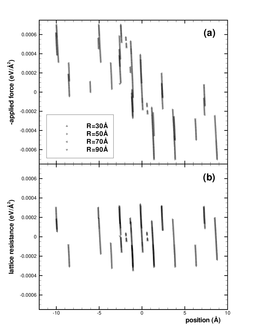
Figure 5: Comparison of (a) the applied force and (b) the corrected lattice resistance for the screw dislocation. The $x$-axis shows the position of the dislocation corresponding to where the measured displacement jump is $b/2$.

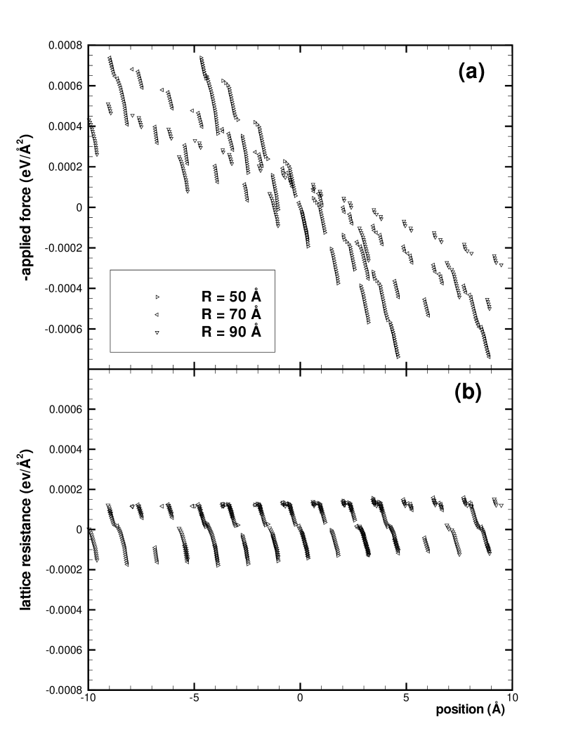
Figure 6: Comparison of (a) the applied force and (b) the corrected lattice resistance for the 30^∘ dislocation. The $x$-axis shows the position of the dislocation corresponding to where the measured displacement jump is $b/2$, adjusted so that the position of the dislocation in the absence of an applied stress is zero.

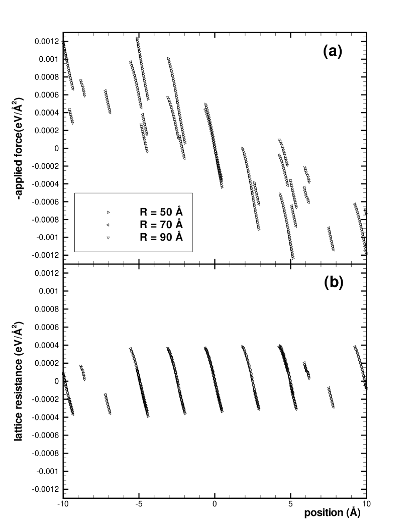
Figure 7: Comparison of (a) the applied force and (b) the corrected lattice resistance for the 60^∘ dislocation. The $x$-axis shows the position of the dislocation corresponding to where the measured displacement jump is $b/2$, adjusted so that the position of the dislocation in the absence of an applied stress is zero.

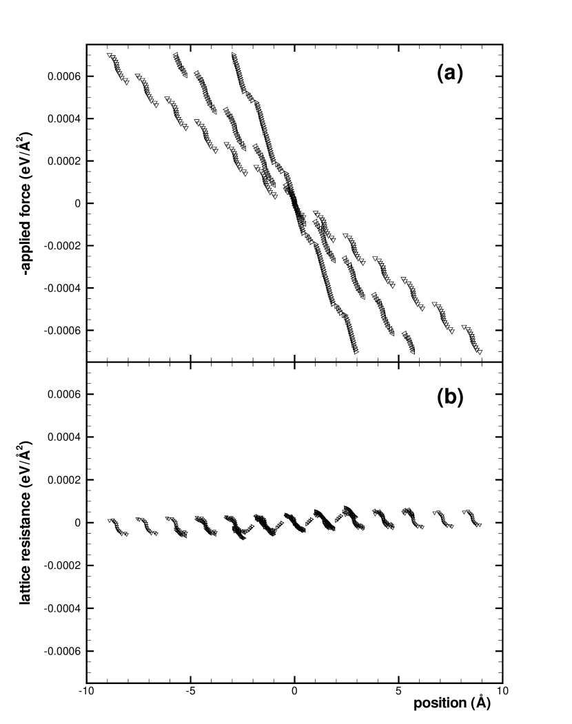
Figure 8: Comparison of (a) the applied force and (b) the corrected lattice resistance for the edge dislocation. The $x$-axis shows the position of the dislocation corresponding to where the measured displacement jump is $b/2$.

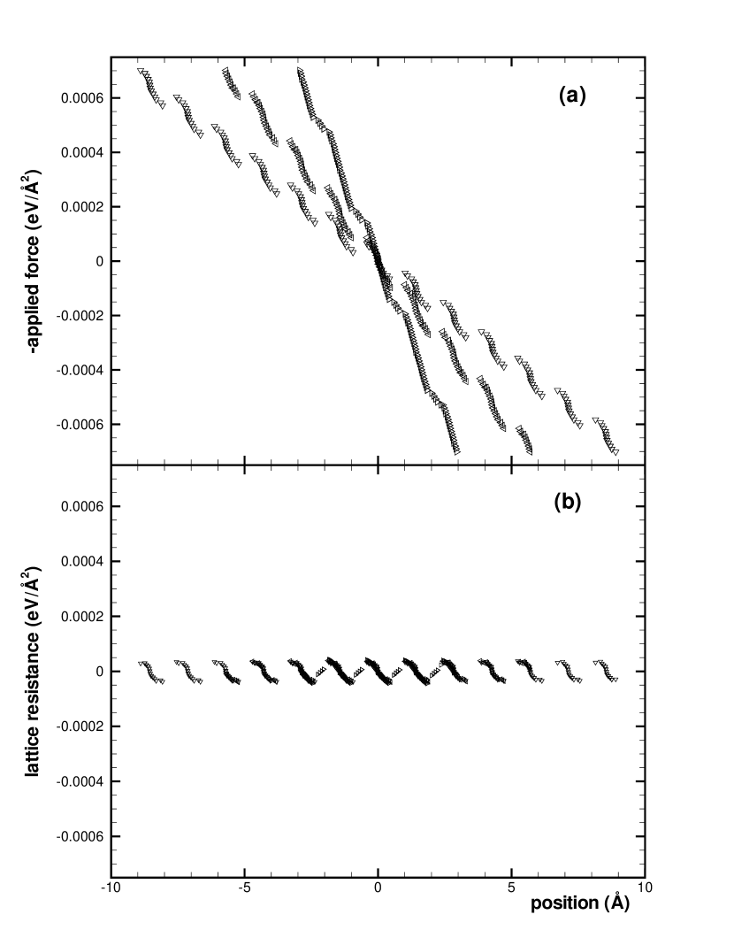
Figure 9: Comparison of (a) the applied force and (b) the corrected lattice resistance for the edge dislocation, where the corrected lattice resistance is based on optimal choice of the boundary force coefficient. The $x$-axis shows the position of the dislocation corresponding to where the measured displacement jump is $b/2$. The adjustment in the boundary force coefficient varies from a 5% reduction in $A$ for $R=50$ Å to a 3% reduction for $R=90$ Å.

One of the assumptions underlying our approach is that the lattice resistance term in equation (9) is periodic in $d$ once the boundary force correction is made. By examining the degree to which our corrected lattice resistance force is indeed periodic, we test the accuracy of our boundary force corrections. (In combination with the assumptions embodied in equation (9), since their failure would also introduce errors.) We can test this visually by graphing the data from one well, offset by the repeat distance, on top of another well. Figures 10, 11, 12, 13, and 14, show the lattice resistance curves formed by plotting all of the wells on top of each other, offsetting each well by an appropriate number of repeat distances. Except for the edge dislocation, the boundary force corrections are computed with the coefficients determined using linear elasticity. figure 14 shows the results for the edge dislocation with the coefficients computed from elasticity. The slight overestimate of $A$ is quite apparent in the scatter. figure 13 shows the same simulation data, but with the boundary-force corrections based on $A$ values for each $R$ chosen to produce the least scatter. The values chosen range from 95% ($R=50$ Å) to 97% ($R=90$ Å) of the elasticity values.

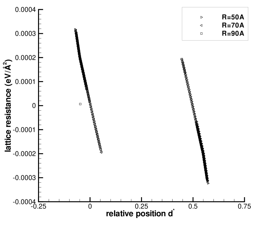
Figure 10: Lattice resistance for the screw dislocation. Position is plotted assuming the expected periodicity of $d_{0}=2.469$ Å. The data is plotted so that data expected to be equal by periodicity lies at the same abscissa. $d^{*}$ is $d/d_{0}$ offset by the integer such that $-0.25<d^{*}<0.75$.

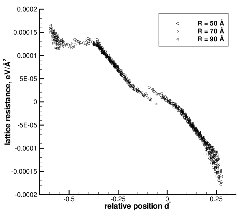
Figure 11: Lattice resistance for the 30^∘ dislocation. Position is plotted assuming the expected periodicity of $d_{0}=1.426$ Å. The data is plotted so that data expected to be equal by periodicity lies at the same abscissa. $d^{*}$ is $d/d_{0}$ offset by the integer such that $-0.65<d^{*}<0.35$.

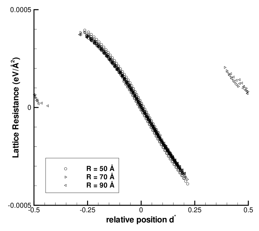
Figure 12: Lattice resistance for the 60^∘ dislocation. Position is plotted assuming the expected periodicity of $d_{0}=2.469$ Å. The data is plotted so that data expected to be equal by periodicity lies at the same abscissa. $d^{*}$ is $d/d_{0}$ offset by the integer such that $-0.5<d^{*}<0.5$.

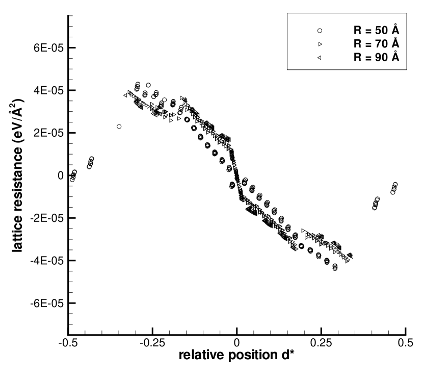
Figure 13: Lattice resistance for the edge dislocation. The $A$ coefficients have been adjusted for best fit. Position is plotted assuming the expected periodicity of $d_{0}=1.426$ Å. The data is plotted so that data expected to be equal by periodicity lies at the same abscissa. $d^{*}$ is $d/d_{0}$ offset by the integer such that $-0.5<d^{*}<0.5$.

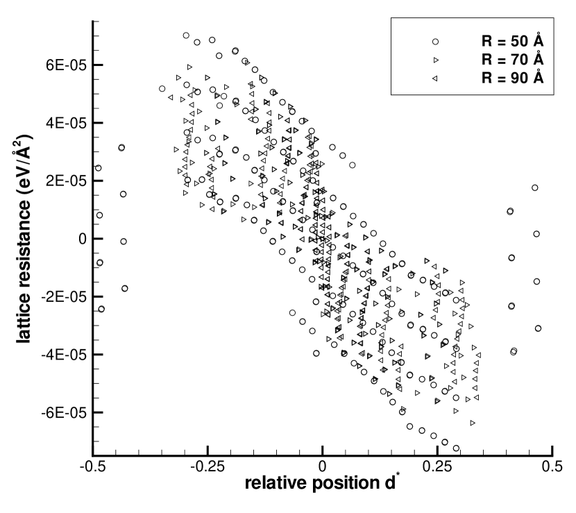
Figure 14: Lattice resistance for the edge dislocation. The $A$ coefficients are from elasticity. Position is plotted assuming the expected periodicity of $d_{0}=1.426$ Å. The data is plotted so that data expected to be equal by periodicity lies at the same abscissa. $d^{*}$ is $d/d_{0}$ offset by the integer such that $-0.5<d^{*}<0.5$.

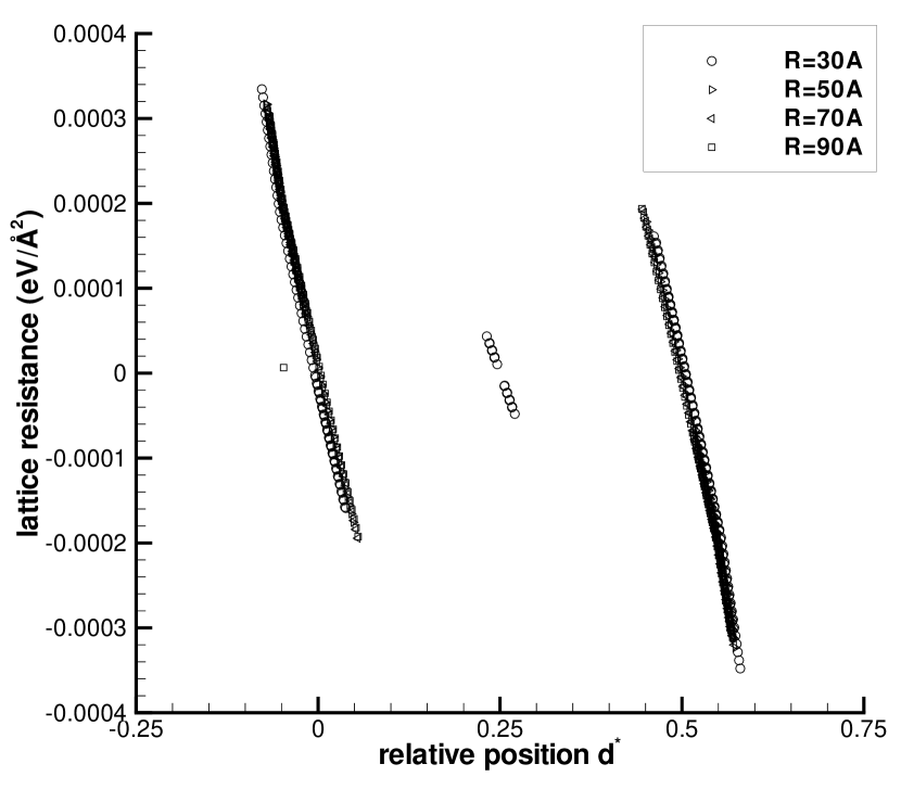
Figure 15: Lattice resistance for the screw dislocation, including additional smaller cell size. Position is plotted assuming the expected periodicity of $d_{0}=2.469$ Å. The data is plotted so that data expected to be equal by periodicity lies at the same abscissa. $d^{*}$ is $d/d_{0}$ offset by the integer such that $-0.25<d^{*}<0.75$.

The lattice resistance curves for the different dislocations are very different, both in shape and in scale. The screw and edge curves show a reflection symmetry that the mixed dislocations do not. This is expected, because the two partials of the edge (screw) dislocation have the same character. In all four plots there is good agreement between different wells for the same radius simulation cell. Except for the edge dislocation, there is also very good agreement between the different size simulation cells. A more significant size effect is apparent in the shape of the curve for the edge dislocation. Because the lattice resistance forces for the edge dislocation have the smallest magnitudes, while the boundary forces being subtracted from the applied force are the largest, some of this discrepancy may simply arise from the fact that the radii used for the simulation cells are effectively smaller for the edge dislocation. In an attempt to shed light on this possibility a screw dislocation run was made in a cell with a radius of 30 Å. figure 15 shows this data along with the other 3 radii. While there is poorer agreement with the other sizes for the 30 Å radius, the shape is unchanged. This suggests that the size dependence of the shape of the curve for the edge dislocation may truly differ from that of the other dislocation studied.

Perhaps the plot for the 60^∘ dislocation looks most reminiscent of the accessible portion of a sinusoidal lattice resistance curve. The 30^∘ dislocations shows considerably more structure. The lattice resistance curve for the screw dislocation, shows two interesting phenomena. First, the form of the force curve implies that the Peierls well depicted is split into two separate sub-wells, separated by a local maximum. Secondly, as the lattice resistance force approaches its maximum there is no softening of the slope. While we admit to finding this latter circumstance somewhat perplexing, it should be borne in mind that the force being plotted is the configurational force on the dislocation, not the actual force on any atom, nor the actual elastic stress at any point.

Our primary purpose here in measuring the lattice resistance curves for the different dislocations is to demonstrate the ability of the boundary force correction scheme proposed in (I) to handle edge and mixed dislocations. As we have measured these curves using a single semi-empirical classical potential, it is perhaps overly optimistic to present these results as a trustworthy guide, even in qualitative terms, to the variation of lattice resistance curves with character of dislocation in real aluminum. On the other hand, our results provide substantial quantitative support for the technique being used to obtain such curves and suggests that this same strategy could be useful in the context of more reliable descriptions of the total energy.

5.1. Peierls Stress

We have measured the Peierls stress, that is the resolved shear stress in the glide direction required to move a dislocation, both with and without boundary corrections. Figures 16, 17, 18 and 19 show the uncorrected and the corrected estimates of the Peierls stress as functions of $1/R^{2}$, for the four dislocaions studied. In these plots we show the resolved applied stress for the simulation step just before the jump as the data point. As an indication of the range that the measurement might fall in because of step size we show, as an error bar, the applied stress step size for the uncorrected-Peierls stress, and an estimate of the effective step size for the corrected-Peierls stress. In each case, the corrected measurements are substantially less affected by the size of simulation cell chosen than the uncorrected measurements. For the screw dislocation, where the Peierls force is relatively large, and the boundary force correction relatively small, the uncorrected results at the larger simulation sizes are similar to the corrected ones. On the other hand, for the edge dislocation, where the boundary forces are larger, and the Peierls force much smaller, the uncorrected values are very different from the corrected ones.

For the lattice resistance curves above, taking data from wells many repeat distances away from the center of the cell, obtaining the agreement shown required care in determining the quadratic term of the boundary force correction, including tuning for the edge dislocation. For measuring the Peierls force using the central well, the boundary force correction is important, but the results are not very sensitive to changes in $A$ of a few percent.

figure 20 shows our results for the Peierls stress in aluminum, as predicted by the Ercolessi and Adams glue potential. We have not made any tests of the sensitivity of these results to the type of potential used, or its details. Nor are we aware of any experimental data or theoretical predictions for the relationship between the Peierls stresses for the edge and screw dislocations in aluminum. Nonetheless, we find it interesting to see a difference as great as a factor of 8 between the screw and edge values in an fcc metal.

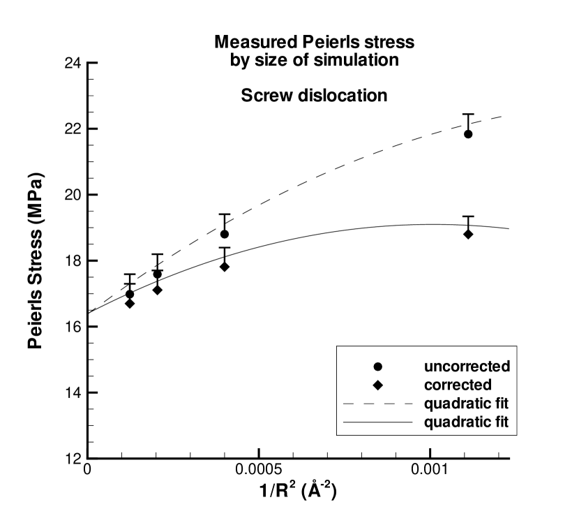
Figure 16: Peierls stress measured with and without boundary force corrections for the screw dislocation. Error bars represent the approximate step size. The fitted curves are suggestive only, and are not proposed as extrapolations to large $R$.

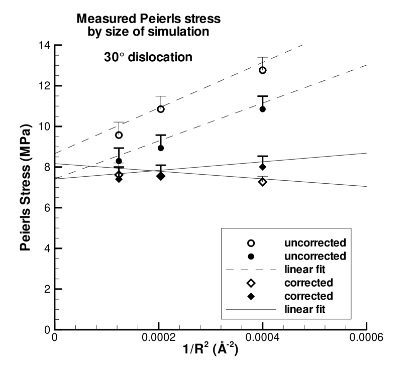
Figure 17: Peierls stress measured with and without boundary force corrections for the 30^∘ dislocation. Open and solid symbols are the two directions of motion. The structure near the maximum on the left side of figure 11 causes some inconsistency between the $R=50$ Å corrected value in that direction and the larger cells. The fitted lines are suggestive only, and are not proposed as extrapolations to large $R$.

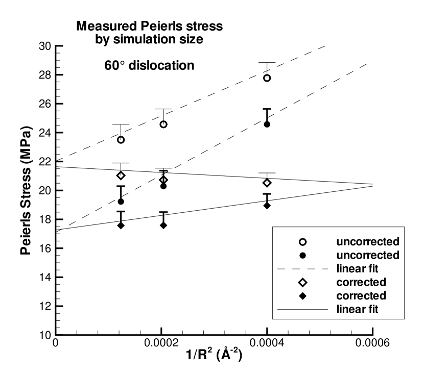
Figure 18: Peierls stress measured with and without boundary force corrections for the 60^∘ dislocation. Open and solid symbols are the two directions of motion. The fitted lines are suggestive only, and are not proposed as extrapolations to large $R$.

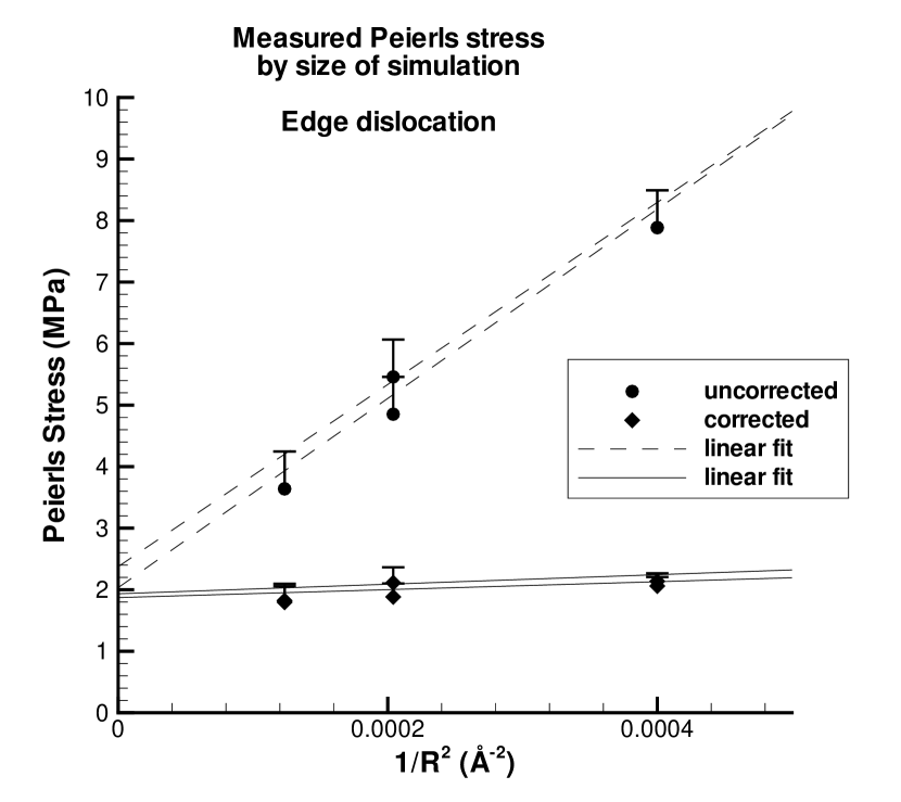
Figure 19: Peierls stress measured with and without boundary force corrections for the edge dislocation. Data for the two directions of motion are shown, but should be equivalent for the edge dislocation. The fitted lines are suggestive only, and are not proposed as extrapolations to large $R$.

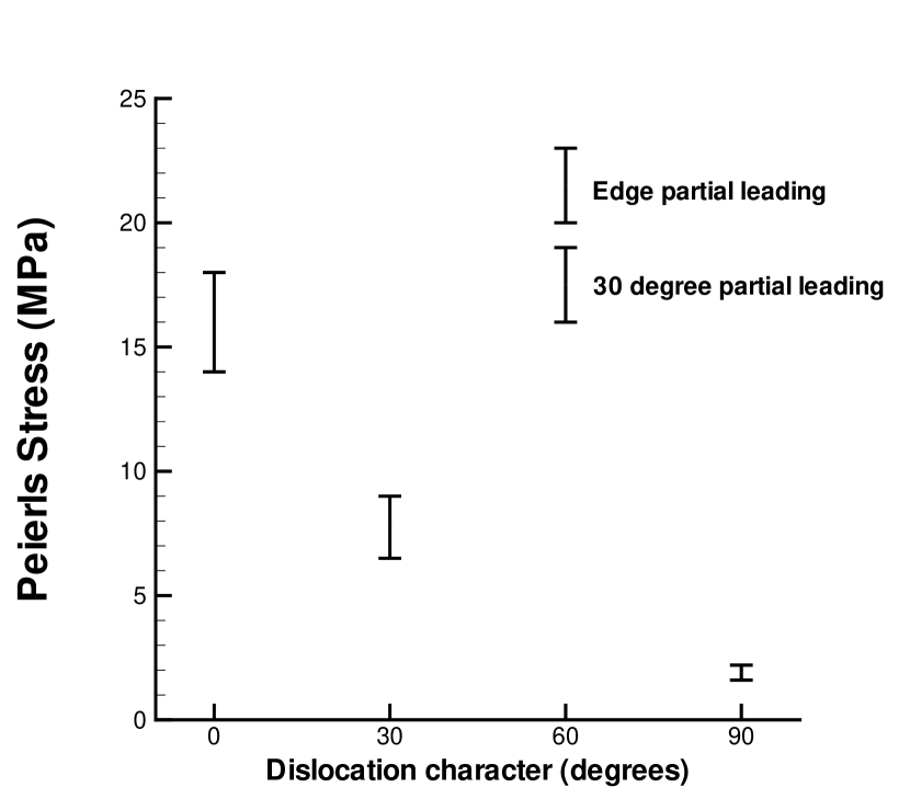
Figure 20: Peierls stress for the different dislocations. The dislocations are labeled by the angle between the line direction and the Burgers vector, with the screw dislocation labeled 0 and the edge dislocation labeled 90. The range shown for each measurement was subjectively determined by examining Figures 16, 17, 18 and 19. For the 60^∘ dislocation the dislocation core is not symmetric with respect to the direction of motion, because one partial has edge character, while the other partial has mixed character. As it moves from one Peierls well to the next it will cross an identical maximum energy in either direction, but as the shape of the hill need not be the same on both sides, the maximum resistance encountered in the two directions differs. In principle the two directions of motion for the 30^∘ dislocation are different, but the data does not show a clear difference in Peierls stress.

J. P. Simmons, et al., measured the Peierls stress of unit ${\frac{1}{2}}a_{0}\{110\}$ dislocations in an ordered $L1_{0}$ structure in several embedded-atom method potentials which were fitted to $\gamma$–TiAl [11]. For their preferred potential they measured the Peierls stress for the four dislocation characters treated in this work. Those Peierls stresses are about a factor of 10 larger than in our material, but the overall qualitative result that the maximum lattice resistance for the screw and $60^{\circ}$ dislocations are significantly larger than those of the edge and $30^{\circ}$ dislocations is similar to what they observed. They ascribed this overall result to the difference in the density of atom planes in the direction of motion, which is a factor of 1.7 higher for the edge and $30^{\circ}$ dislocations. They support this suggestion based on the Peierls-Nabarro model, using the work of Weertman and Weertman [18]. The suggestion that this is the primary element in the overall differences between the different dislocation characters is to some degree supported by the fact that we see, in an fcc potential with much smaller Peierls stresses, the same type of difference between the two dislocations with the larger distance between atom planes in the direction of motion and the two with the smaller distance, but the relationships between the Peierls stresses of dislocations with the same distance between atomic planes are not similar between the two cases. However, in our case the Peierls stress for the $30^{\circ}$ dislocation exceeds that of the edge dislocation by almost as much as the difference between the Peierls stresses for the $30^{\circ}$ dislocation and the screw dislocation, and so the difference in atomic plane density does dominate the results as clearly as in the Simmons et al. results.

Our result for the Peierls stress of the screw dislocation is shown as 14-18 MPa, and is 20% or more smaller than the estimate in (I) for the same material, using essentially the same approach. To some extent this involves the inclusion of a larger disk size than in (I). There is also a significant effect in this case from the use of the linear elastic solution for the two Shockley partials in generating the positions of the atoms in the fixed ring, as opposed to the use in (I) of the linear elastic solution for the perfect dislocation.

Bulatov, et al., have also measured the Peierls stress of the screw and $60^{\circ}$ degree dislocations for the same Ercolessi and Adams potential for Aluminum, using fully periodic boundary conditions [4]. They report a Peierls stress of 82 MPa for the screw dislocation, and 47 MPa for the $60^{\circ}$ degree dislocation. These results are substantially higher than ours. They also exceed all of our uncorrected estimates, which should definitely be overestimated because of the boundary repulsion. We can see no reason why our estimates should be so substantially underestimated as the Bulatov, et al. figures would suggest. Our results however, as discussed above, are for a particular stress state, chosen to provide equal Peach-Kohler forces on the two partials.

6. Conclusions

When simulations are performed of dislocations in finite-size simulation cells, boundary forces will often be important. One approach to correcting for boundary forces is that proposed by Shenoy and Phillips in (I). We have shown how that method can be extended to edge and mixed dislocations, and to general cell shapes, and have applied the technique to the measurement of the lattice resistance curves and Peierls stresses of four mobile dislocations in fcc aluminum. In addition, we have turned the usual elastic arguments concerning the nature of configurational forces on their side and introduced a purely atomistic scheme for computing such boundary forces. A second outcome of our analysis is the recognition of the consistency of the boundary forces obtained using either elasticity or atomistic analysis. We also note that our results are illustrative in that they signify a large degree of control over the various contributions to the total energy in a finite size system.

Our methods assume that the total configurational force on a dislocation can be divided into three parts,

• An applied force given by the Peach-Kohler formula.

• A periodic lattice resistance force, independent of position within the simulation cell, and independent of cell radius.

• A boundary-effect force which is a function of $d/R$. For the case of two Shockley partials the boundary-effect force also depends on $s/R$, where $s$ is half the partial separation.

The data from our simulations support this assumption, except that for the edge dislocation the shape of the measured lattice resistance force curve has some dependence on the size of the simulation cell. In addition we find that a linear elastic computation of the boundary-force function gives reasonable results, which were adequate for our purposes for all of the dislocations except the edge. While we have considered the dependence of $A$ on $s/R$ caused by the extension (treated as dissociation) of the dislocation, and have considered the higher order coefficients $B$ and $C$ as well, these are small effects, and we expect that in many cases simply using the value of $A$ computed for a perfect dislocation will provide a reasonable estimate of the boundary force. We also find that both the shape of the lattice resistance landscape, as well as the magnitude of the Peierls stress, depend strongly on the dislocation character.

From the perspective of future applications of ideas like those introduced here, we note that we foresee at least two fertile avenues for further work. First, within the context of the type of simple geometries considered here, we argue that the analysis of boundary forces could be a potentially useful way of turning the disadvantage of small system sizes used in first-principles simulations of complex systems into a means of precise control of the boundary conditions used in such simulations. Perhaps more importantly, we view our analysis as a first step towards the more judicious management of boundary conditions associated with complex three-dimensional geometries involving dislocations. In particular, recent work on both dislocation junctions [19, 20, 21] and cross-slip [22, 23] are a significant first step towards informing higher-level dislocation dynamics simulations of plasticity on the basis of atomic-level understanding of the “unit processes” involving dislocations. One of the key challenges faced in effecting calculations that are quantitatively meaningful is combatting the spurious effects induced by the presence of unwanted nearby boundaries. The present work offers the possibility of finite-element based, linear elastic calculations of the effects of such boundaries, thus clearing the way for substantive quantitative insights into these processes.

Appendix A — Partial Splitting

For our model aluminimum system all of the easy-glide dislocations split (approximately) into Shockley partials. The width of the partial dislocations is similar to their separation distance, so that their core regions overlap to some extent. While this means that there is no region on the slip plane that is a close approximation to a stacking fault, the elasticity model of two unextended Shockley partials separated by a stacking fault remains useful.

Image Solution

While we are unable to use the image solution to handle the actual Shockley partials of the screw dislocation, which include edge components, it is possible to use it for the simpler case of pure screw partials, each with a Burgers vector of one-half $b$, at fixed separation. We hope that this simplified model will at least indicate the nature of the extra subtlety in the boundary force as a result of the splitting of the dislocation into partials. There are two possible boundary conditions to consider. One is where the fixed displacements at the boundary are those of a single screw dislocation at the center of the cell. In the other case we compute the fixed displacements based on the two partial dislocations, with the center of the cylinder located half-way between the two partials.

Letting $s$ be one-half the partial separation, the partials are located at $d+s$ and $d-s$. When the boundary conditions are those of a single dislocation, only two image dislocations are needed. These are screw dislocation at $L=\frac{R^{2}}{d+s}$ and $L=\frac{R^{2}}{d-s}$, each with Burgers vector $b/2$. (When $d=\pm s$, one of the partials is at the center of the disk, and its image dislocation is not needed.) The force on the dislocation is now

$$F/l=-\frac{\mu(b/2)^{2}}{2\pi}\left[\frac{1}{\frac{R^{2}}{d+s}-(d+s)}+\frac{1}{\frac{R^{2}}{d-s}-(d+s)}+\frac{1}{\frac{R^{2}}{d+s}-(d-s)}+\frac{1}{\frac{R^{2}}{d-s}-(d-s)}\right].$$ (39)

While the result of integrating this to obtain the energy is not particularly complicated, neither is it particularly enlightening. Letting $c=s/R$, and treating the partial splitting as making the terms in our expansion of the boundary energy depend on $c$, we obtain

$$A =2\pi\frac{(1+c^{4})}{(1-c^{2})^{2}(1+c^{2})}$$ (40)

$$=2\pi\left[1+c^{2}+3c^{4}+O(c^{6})\right]$$ (41)

$$B =\pi\left[1+4c^{2}+O(c^{4}).\right]$$ (42)

[The result for A under these conditions was shown in figure A 1 of (I).]

When the boundary displacements are computed using the partials (which mimics the boundary conditions of our simulations) the situation is slightly more complicated. The boundary conditions are the displacements resulting from one partial at $s$ and one at $-s$. The actual dislocations are at $d+s$ and $d-s$. A $+b/2$ dislocation at $s$ and one at $R^{2}/s$ combine to give the boundary displacements of a $+b/2$ dislocation at the center. A $+b/2$ dislocation at $d+s$ and one at $R^{2}/(d+s)$ also combine to give the boundary displacements of a $+b/2$ dislocation at the center. Thus the actual $+b/2$ partial at $d+s$ together with a $+b/2$ dislocation at $R^{2}/(d+s)$ and a $-b/2$ dislocation at $R^{2}/s$ will combine to produce the displacements of the $b/2$ dislocation at $s$. Handling the other partial in the same way, we then have four image dislocations, two of like Burgers vector as the actual partials, and two with equal and opposite Burgers vectors. There are now eight terms contributing to the configurational force on the dislocation computed based on the image dislocations, and we have

$$F/l=-\frac{\mu(b/2)^{2}}{2\pi}\left[\frac{1}{\frac{R^{2}}{d+s}-(d+s)}\right. + \frac{1}{\frac{R^{2}}{d-s}-(d+s)}$$

$$\mbox{}-\frac{1}{\frac{R^{2}}{s}-(d+s)} - \frac{1}{\frac{R^{2}}{-s}-(d+s)}$$

$$\mbox{}+\frac{1}{\frac{R^{2}}{d+s}-(d-s)} + \frac{1}{\frac{R^{2}}{d-s}-(d-s)}$$

$$\mbox{}-\frac{1}{\frac{R^{2}}{s}-(d-s)} - \left.\frac{1}{\frac{R^{2}}{-s}-(d-s)}\right].$$ (43)

For these boundary conditions we have

$$A =2\pi\left[1+3c^{4}+O(c^{6})\right]$$ (44)

$$B =\pi\left[1+4c^{2}+O(c^{4})\right].$$ (45)

Aside from the usefulness of this result as a benchmark in testing our FEM computations, the point of interest is that the highest order correction to the boundary force as a result of partial splitting, which is of order $ds^{2}/R^{4}$, is zero when the fixed displacements are computed based on the partials. For the more general case, with anisotropic elasticity, and non-screw dislocations this term is no longer zero, but it is small, and varies in sign between the different dislocations.

Subtracting, rather than adding, the forces on the two partials, and dividing by two, we obtain the extra force (per unit length) applied to the “spring” connecting the two partials because of the boundary conditions. This may be of some use in estimating how large a cylinder is needed to avoid distortions in the partial separation, assuming the stacking fault energy is available. For the case where the boundary displacements are based on a perfect dislocation, there is a force even when the dislocation is at the center of the disk. The result is that the “spring” is compressed by a force on each end of

$$F_{\mbox{\scriptsize C}}/l=\frac{\mu(b/2)^{2}}{2\pi}\frac{2s^{3}}{R^{4}-s^{4}},$$ (46)

at the nominal separation of $2s$. This would then be partially relaxed by a reduction in the separation. Including the overall displacement of the dislocation, while still keeping the partial separation fixed, and keeping only terms to order $R^{-4}$ the compression is

$$F_{\mbox{\scriptsize C}}/l\approx\frac{\mu(b/2)^{2}}{2\pi}\left[\frac{2s^{3}}{R^{4}}+\frac{2sd^{2}}{R^{4}}\right].$$ (47)

If the boundary displacements are instead based on the two “partials”, the force on each end of the “spring” is

$$F_{\mbox{\scriptsize C}}/l\approx\frac{\mu(b/2)^{2}}{2\pi}\frac{2sd^{2}}{R^{4}},$$ (48)

to the same approximation. While these results are for the unphysical case of an isotropic screw dislocation split into pure screw partials, it should be a correct guide to the scaling of the dominant term in the expansion.

Elasticity Solution

In this section we extend equation (32) to the case where the dislocation is split into two (Shockley) partials. The partials have Burgers vectors adding up to the Burgers vector of the perfect dislocation

$${{\bf b}}^{(l)}+{{\bf b}}^{(r)}={{\bf b}}^{(f)},$$ (49)

where a superscript l(r) will refer to the left(right) partial, and a superscript f will refer to the full dislocation. The partials have the same line direction as the perfect dislocation, and, for the case of Shockley partials, the Burgers vectors of the partials lie in the same slip plane that the Burgers vector of the perfect dislocation does.

We apply the sextic formulation of Eshelby, et. al [12, 13], as applied to the case of partial dislocations by Teutonico [14]. We follow the treatment of Hirth and Lothe [15] explicitly, varying the notation just enough to include the superscripts for the two partials and the perfect dislocation.

The coordinate axes are chosen so that $\hat{x}_{3}$ is the line direction and $\hat{x}_{2}$ is the perpendicular to the slip plane. This means that $\hat{x}_{1}$ is the direction in which the movement of dislocation is measured, and the direction in which the partial separation is measured. We choose $s$ as half the distance between the two partials, and assume it to be independent of $d$. The left and right partials are therefore located at $d-s$ and $d+s$ respectively. (Notice that this choice of axes is different from that used elsewhere in this paper.)

We wish to evaluate

$${\Delta E^{a}}={\frac{1}{2}}{\int_{\partial M_{s^{\prime}}}}{{\bf t}}_{P}\cdot{[[{{\bf u}}_{P}]]}{\,\mbox{d}}S-{\frac{1}{2}}{\int_{\partial M_{s}}}{{\bf t}}_{O}\cdot{[[{{\bf u}}_{O}]]}{\,\mbox{d}}S.$$ (50)

We write

$$\frac{1}{l}{\frac{1}{2}}{\int_{\partial M_{s}}}{{\bf t}}_{O}\cdot{[[{{\bf u}}_{O}]]}{\,\mbox{d}}S ={\frac{1}{2}}\int_{-R}^{-s-r_{c}}\left\{{{\bf t}}_{O}^{(l)}(x_{1})+{{\bf t}}_{O}^{(r)}(x_{1})\right\}\cdot{{\bf b}}^{(f)}dx_{1}$$

$$+{\frac{1}{2}}\int_{-s+r_{c}}^{s-r_{c}}\left\{{{\bf t}}_{O}^{(l)}(x_{1})+{{\bf t}}_{O}^{(r)}(x_{1})\right\}\cdot{{\bf b}}^{(r)}dx_{1}$$ (51)

$$\frac{1}{l}{\frac{1}{2}}{\int_{\partial M_{s^{\prime}}}}{{\bf t}}_{P}\cdot{[[{{\bf u}}_{P}]]}{\,\mbox{d}}S ={\frac{1}{2}}\int_{-R}^{d-s-r_{c}}\left\{{{\bf t}}_{P}^{(l)}(x_{1})+{{\bf t}}_{P}^{(r)}(x_{1})\right\}\cdot{{\bf b}}^{(f)}dx_{1}$$

$$+{\frac{1}{2}}\int_{d-s+r_{c}}^{d+s-r_{c}}\left\{{{\bf t}}_{P}^{(l)}(x_{1})+{{\bf t}}_{P}^{(r)}(x_{1})\right\}\cdot{{\bf b}}^{(r)}dx_{1}.$$ (52)

Rewriting equations (51) and (52) in terms of ${{\bf t}}^{(l)}(x_{l})$ where $x_{l}$ is measured from the location of the left partial, and ${{\bf t}}^{(r)}(x_{r})$ where $x_{r}$ is measured from the location of the right partial, and taking the difference we have

$${\Delta E^{a}}/l={\frac{1}{2}}\int_{-R-d+s}^{-R+s}{{\bf t}}^{(l)}(x_{l})\cdot{{\bf b}}^{(f)}dx_{l}+{\frac{1}{2}}\int_{-R-d-s}^{-R-s}{{\bf t}}^{(r)}(x_{r})\cdot{{\bf b}}^{(f)}dx_{r}.$$ (53)

The stresses within the sextic formulation are computed as follows using the notation of [15] to which the reader is referred for the derivations.

Define

$$a_{ik}\equiv c_{i1k1}+(c_{i1k2}+c_{i2k1})p+c_{i2k2}p^{2},$$ (54)

for $p$ an arbitrary complex number. We need solutions of the equations

$$a_{ik}A_{k}=0,\hskip 20.00003pti=1,2,3,$$ (55)

which can only hold if $\det([a_{ik}(p)])=0$. This sixth degree real polynomial equation can be shown to have no real roots, so that its solutions are three pairs of complex conjugates, and pick $p_{(1)}$, $p_{(2)}$ and $p_{(3)}$ to be the three solutions with positive imaginary parts. We let ${\bf A}(n)$ be the solution of equation (55) corresponding to $p_{(n)}$. We also define a three-tensor

$$B_{ijk}(n)\equiv c_{ijk1}+p_{(n)}c_{ijk2},\hskip 20.00003ptn=1,2,3.$$ (56)

Notice that $p_{(n)}$, ${\bf A}(n)$ and ${\bf B}(n)$ depend on the line direction of the dislocation and the slip plane, but not on the Burgers vector, so they are applicable to the perfect dislocation and to the two partials.

We now define, depending on the Burgers vector ${{\bf b}}$, three complex numbers $D(n)$ by the six equations

$$\Re\left[{\sum_{n=1}^{3}}A_{k}(n)D(n)\right] =b_{k}$$

$$\Re\left[{\sum_{n=1}^{3}}B_{k2l}(n)A_{l}(n)D(n)\right] =0,$$ (57)

Where $\Re(z)$ is the real part of $z$. This does involve the Burgers vector, so we have $D^{(l)}(n)$, $D^{(r)}(n)$, and $D^{(f)}(n)$. However the equations are linear in ${{\bf b}}$ and $D$, so that we have

$$D^{(l)}(n)+D^{(r)}(n)=D^{(f)}(n).$$ (58)

We now have [15]

$$\sigma_{ij}^{(\#)}(x_{(\#)},0,z)=\frac{-1}{2\pi x_{(\#)}}\Im\left[{\sum_{n=1}^{3}}B_{ijk}(n)A_{k}(n)D^{(\#)}(n)\right],$$ (59)

where $(\#)$ is $(l)$, $(r)$ or $(f)$, the relevant dislocation is situated at $x_{(\#)}=0$, and $\Im(z)$ is the imaginary part of $z$. Since our slip plane is perpendicular to $x_{2}$, we have

$$t^{(\#)}_{i}=\sigma_{i2}=\frac{-1}{2\pi x_{(\#)}}\Im\left[{\sum_{n=1}^{3}}B_{i2k}(n)A_{k}(n)D^{(\#)}(n)\right].$$ (60)

We now define

$$F_{l} =\frac{1}{4\pi}\Im\left[{\sum_{n=1}^{3}}b^{(l)}_{i}B_{i2k}(n)A_{k}(n)D^{(l)}(n)\right],$$ (61)

$$F_{r} \mbox{\ similarly},$$ (62)

$$F_{\mbox{\scriptsize int}} =\frac{1}{4\pi}\Im\left[{\sum_{n=1}^{3}}b^{(l)}_{i}B_{i2k}(n)A_{k}(n)D^{(r)}(n)\right]$$ (63)

$$=\frac{1}{4\pi}\Im\left[{\sum_{n=1}^{3}}b^{(r)}_{i}B_{i2k}(n)A_{k}(n)D^{(l)}(n)\right],$$ (64)

where the last equality holds because the interaction forces between the partials must be equal and opposite. Thus we have

$${{\bf t}}^{(l)}\cdot{{\bf b}}^{(l)} =-2F_{l}/x_{l}$$ (65)

$${{\bf t}}^{(r)}\cdot{{\bf b}}^{(r)} =-2F_{r}/x_{r}$$ (66)

$${{\bf t}}^{(r)}\cdot{{\bf b}}^{(l)} =-2F_{\mbox{\scriptsize int}}/x_{r}$$ (67)

$${{\bf t}}^{(l)}\cdot{{\bf b}}^{(r)} =-2F_{\mbox{\scriptsize int}}/x_{l}.$$ (68)

From equation (53) we have

$${\Delta E^{a}}/l =-\left(F_{l}+F_{\mbox{\scriptsize int}}\right)\int_{-R-d+s}^{-R+s}x^{-1}dx-\left(F_{r}+F_{\mbox{\scriptsize int}}\right)\int_{-R-d-s}^{-R-s}x^{-1}dx$$ (69)

$$=\left(F_{l}+F_{\mbox{\scriptsize int}}\right)\log\left(\frac{R+d-s}{R-s}\right)+\left(F_{r}+F_{\mbox{\scriptsize int}}\right)\log\left(\frac{R+d+s}{R+s}\right),$$ (70)

which reduces to equation (32), as it should, on setting $s$ equal to zero.

The forms for ${\Delta E^{b}}$ and ${\Delta E^{c}}$ at equations (33) and (36) are directly applicable to the case where the dislocation is split into partials, so equation (70) is the only additional formula needed for the elasticity computation.

References

- [1] V. B. Shenoy and R. Phillips, Phil. Mag. A 76, 367 (1997).
- [2] F. Ercolessi and J. B. Adams, Europhys. Lett. 26, 583 (1994).
- [3] S. Rao, C. Hernandez, J. P. Simmons, T. A. Parthasarathy, and C. Woodward, Phil. Mag. A 77, 231 (1998).
- [4] V. V. Bulatov, O. Richmond, and M. V. Glazov, Acta Mater. 47, 3507 (1999).
- [5] V. V. Bulatov, S. Yip, and A. S. Argon, Phil. Mag. A 72, 453 (1995).
- [6] M. S. Daw, M. I. Baskes, C. L. Bisson, and W. G. Wolfer, in Modelling Environmental Effects on Crack Growth, edited by R. H. Jones and W. W. Gerberich (The Metallurgical Society, Warrendale, PA, 1986), p. 99.
- [7] M. S. Daw, S. M. Foiles, and M. I. Baskes, Mater. Sci. Rep. 9, 251 (1993).
- [8] D. Rodney and G. Martin, Phys. Rev. Lett. 82, 3272 (1999).
- [9] D. Rodney and G. Martin, Phys. Rev. B 61, 8714 (2000).
- [10] J. P. Hirth and J. Lothe, Theory of Dislocations, 2nd ed. (John Wiley & Sons, New York, 1982).
- [11] J. P. Simmons, S. I. Rao, and D. M. Dimiduk, Phil. Mag. A 75, 1299 (1997).
- [12] J. D. Eshelby, W. T. Read, and W. Shockley, Acta Met. 1, 251 (1953).
- [13] A. J. E. Foreman, Acta Met. 3, 322 (1955).
- [14] L. J. Teutonico, Acta Met. 11, 1283 (63).
- [15] See ref. [10], pp 436-445.
- [16] M. S. Duesbury, in Dislocations in Solids, edited by F. R. N. Nabarro (Elsevier, Amsterdam, 1989), Vol. 8, p. 67.
- [17] R. Miller and R. Phillips, Phil. Mag. A 73, 803 (1996).
- [18] J. Weertman, J. R. Weertman, and D. M. Dimiduk, Elementary Dislocation Theory (Oxford University Press, Oxford, 1992).
- [19] V. Bulatov, F. Abraham, L. Kubin, B. Devincre, and S. Yip, Nature 391, 699 (1998).
- [20] S. J. Zhou, D. L. Preston, P. S. Lomdahl, and D. M. Beazley, Science 279, 1525 (1998).
- [21] D. Rodney and R. Phillips, Phys. Rev. Lett. 82, 1702 (1999).
- [22] T. Rasmussen, K. W. Jacobsen, T. Leffers, and O. B. Pedersen, Phys. Rev. B 56, 2977 (1997).
- [23] T. Rasmussen et al., Phys. Rev. Lett. 79, 3676 (1997).